Effects of In-Kind transfers on female labor supply: evidence from the food supply program comedores comunitarios

(1)

Effects of In-Kind transfers on female labor supply: Evidence

from the food supply program

Comedores Comunitarios

Paul Andr´es Rodr´ıguez Lesmes

February 9, 2011

Abstract

The literature argues that in-kind transfers may have a positive effects on labor supply. In this paper we use a food and nutrition program implemented in Bogota

(Comedores Comunitarios) to shed light on this issue. The program gives poor people

living near dining rooms, one free meal per-day. Using a matching approach with Encuesta de Calidad de Vida 2007 cross-section survey data, both positive and negative significant effects on female labor supply were found for different groups of women (differing in age, household composition and access to social networks). These results are relevant to understand the heterogenous work incentives generated when applying this type of program.

Keywords food and nutrition programs, female labor supply, in-kind transfers, col-lective decision.

JEL codesD12, H42, I38, J22.

1 Introduction

Fighting poverty may involve many instruments and there is no consensus about the best program design. One of the main issues is whether in-kind or cash transfers should be used. In some cases, an in-kind transfer is preferred as it enables the policy-designers to fix receptors consumption bundles. For instance, the Government can be sure of the quality of a lunch, in terms of nutrients and calories, by giving it directly rather than giving its equivalent in cash. Even though this might drive to an inefficient allocation of resources, additional consequences may arise. One of the most important is the distortion of labor supply decisions. Modifications on labor supply may affect long-term consumption paths, tax revenues and imply social costs. This work studies the effect on female labor supply of an in-kind food supply program in Bogota, Colombia.

Experience suggests that female labor supply might react more to a food supply pro-gram than men. First, labor supply is usually more elastic for females than for males 1_.

(2)

Second, food related activities in Colombian families are usually part of women’s role in the household. In consequence, they might be the main beneficiaries of the program since it not only improves the quality of their food but it might also provide them some time left.

In order to improve future in-kind programs design, it is important to know if such programs alter labor supply. Additionally, it is also important to acknowledge the factors that enhance or inhibit those effects. In this article, we address these questions for the specific case of Comedores Comunitarios program in Bogota’s beneficiaries: Is the female labor supply affected by the program?

In this paper we show that the effects of the Comedores Comunitarios Program on female labor supply are heterogeneous. When we analyze the impact at an aggregate level, results are small and similar to those found in the previous literature. However, this changes when specific household groups are analyzed. A positive and significant effect on labor market participation is found (additional 5 pp.) for married women who live with other household members. The impact is positive and bigger for older women (about 11 pp. for women between 47 and 55 years old) but it is negative for younger (fewer 9 pp. for those between 15 and 27 years old).Other characteristics like belonging to a social network, having additional assistance from other programs, living in a larger household, or being a wage earner or a self-employed also causes different effects.

The Comedores Comunitarios (communitarian dining rooms) is a program where a

public dining room provides a daily meal to its beneficiaries in Bogotá (Colombia) city since 2004. They are selected by local committees and must fulfill some participation requirements. The program’s main objective is to supplement nearly half of the total calories and nutrients needed by a person per day. This program gives us the opportunity to analyze an in-kind transfer program where individuals cannot resell the provided good (i.e. the in-kind transfer cannot be converted into a cash transfer). In particular, the effect of such kind of program on female labor supply in a sample from 2007 is considered here. As far as we know, this is the first article that does an impact evaluation for this program. The program was described and summarized by Núñez and Cuesta (2007), but no causal inference was done.

Given the current information, it is not possible to identify individual attendance to the program. Therefore, a wider concept of treatment is used. As the transmission channel involves household level decisions, a woman is considered as treated if any member of their household has attended a dining room. Hence, a composite effect is taken into

and Altonji and Blank (1999). However, there are not clear results about the elasticity of Colombian female labor supply. Robbins and Salinas (2007) observed an increase in Latin-American female labor supply despite the stability of real wages, as part of a global tendency during the second half of XX century.

(3)

account: a direct effect, the individual access to the food, and an indirect effect due to the participation of other household members. The in-kind transfer has two components: the food as a physical good and the time not spent preparing food. The interdependence of each household member budget restrictions must be taken into account: if the income of one member grew or his expenses were reduced, the consumption patterns of the other members are likely to change. This notion leads this research to analyze female labor supply effects in different household structures.

To obtain our results we measure the average treatment effect on the treated (ATT). For this purpose, we need to construct the counterfactual for the treatment group on participation and number of working hours. A counterfactual represents what would have happened if a treated woman was not treated. In order to reliably measure the impact of the program over its beneficiaries, the counterfactual units must be as similar as possible to the treated units. This was done by implementing the matching methodology. It selects a non-treated subset which is as similar as possible to the treated women group. The ATT is the difference in labor supply between the averages of the outputs between the treated units and their counterfactuals units. In particular, the applied matching method is the

nearest neighborhood Mahalanobis metric matching within calipers defined by propensity

score. This procedure and why it was selected will be explained in detail in section 4. The available information which includes treated and not treated units –controls- come from the cross section quality of life survey for Bogot´a in 2007, Encuesta de Calidad de Vida

Bogot´a 2007 (ECV07), done by the Colombian Bureau of Statistics (DANE).

The average effects on labor supply of food supplement programs are usually small and often insignificant. The most studied program is the Food Stamp Program (FSP) in USA. Fraker and Moffitt (1988) estimate that FSP reduces labor supply of single mothers. Hoynes and Schanzenbach (2007) found a similar effect but not significant. Hagstrom (1996) found that FSP has less effect on married couples than on single persons. Skoufias and Gonzalez-Cossio (2008) analyzed a food support program in Mexico and found no effects on both cash and in-kind transfers over labor supply. However, they found effects on time allocation between agricultural and nonagricultural activities. Bingley and Walker (2008) studied the effect of UK’s in-kind food transfers on single mothers labor supply. They found that even though those programs are conditional on working hours, they have little effect on promoting part-time work. This work addreses the same problem but also considering additional variables (apart from family composition) that might induce different reactions of labor supply.

(4)

2 In-kind transfers, cash transfers and labor supply

Currie and Gahvari (2007) argue that economists usually consider kind transfers as in-efficient solutions in terms of redistribution policy compared to cash transfers. In-kind transfers restrict the portfolio decisions of beneficiaries while they may always receive an equivalent in money such that they can choose their prefered consumption levels. How-ever, there are paternalistic arguments to defend such policies2. Essentially, the argument appeals to the presence of an externality: one group takes specific decisions for another group that the second would not take alone.

The link between female labor supply and in-kind transfers is determined by the collec-tive nature of labor supply decision. By affecting consumption of any household member, the program may change labor supply of other household members. We can think that there is a familiar budget restriction that includes food, leisure and anum´erairegood. Each individual in the household makes his choice given an individual restriction that includes a sharing rule (Chiappori, 1992). That is, the amount of his own income that would be given or received depending on all members income. Thus, in the short run the program affects the budget restriction by modifying both food and work force endowments. As a result, families may change their optimal elections in num´eraire consumption and labor supply for each member of the household. As they do not need to pay for food, they can spend the free money either on consumption or leisure. Similarly, as they do not need to cook, that free time can be used in other activities. The expected sign of the effect on labor supply can be positive, negative or null. It depends on household composition and other covariates that might affect the sharing rule and the valuation for food assistance. We turn to the analyisis of this effect.

It is possible to define a utility function for women depending on leisure, L, food consumption, F, and a num´eraire, C, all of them normal goods: U(L, F, C). They must undertake a budget restriction:

wL+C+pB≤w(T −H) +φ(m,W₎ ₍₁₎

The woman’s wage is w and it is a component of a vector including all household wages W_. _T _{is the available time for leisure and work. Work is divided in two activities:} remunerated work,l, andH which is the amount of time devoted to tasks related to food preparation (ie. cooking, buying supplies, etc.): T = L+l+H. There is a household non-labor incomem, that with wages, jointly define the exogenous sharing rule φ(m,W_). Food consumption can be obtained both from household work, bought from the market,

B, and from the in-kind transfer G, so F =f(H) +B+G. It is important to introduce

2_{The relation between welfare programas and labor supply has been summarized by Moffitt (2002)}

(5)

another restriction: B > 0: transferred food can be topped up but cannot be sold in a secondary market. The optimal labor supply depends on wage, exogenous income and the in-kind amount transferred.

The impact of the program on the labor supply comes from the sign of ∂l_∂G∗. The direction of the overall effect is not straightforward. We must take into account the different scenarios: first, is B = 0? That is, does the program gives the household more or better food than the one they would buy or prepare without the program? If not, the women may buy additional food for her household or invest more of her time in preparing it so the transfer will be equal to a lump sum transfer of value pG. On the other case, if food preparation and leisuire are substitutes, the total effect could be either positive or negative (Leonesio, 1988)3. Second, there is a time allocation effect: as G increases F, H could be reduced to use either on L or l. The free time could be spent either in additional working hours, that is, on increasing thenum´eraire consumption, or in “leisure” activities like childcare. Note that the sharing rule might be relevant to determine the income effect and therefore the sign of the effect.

Household composition and women covariates may lead to different effects on sign and intensity. For instance, the presence or not of small children on the household might drive to different results: the more children, the more “leisure” time is requiered by the women; but also more resources are needed for consumption. In this case, we cannot say anything a priori. Consequently, these kind of covariates must be taken into account. Additionally, sharing rule may be different for single and married women, but also between married women with and without children. A single woman may prefer more leisure than additional consumption whereas a single mother may value additional consumption for her children more (as her income is more likely to be the unique resource source). Household decision models, from Becker (1973) to Chiappori (1992), shows that household related variables are important as women share their income with their husbands, children and other relatives. Therefore, in our work it is important to differentiate between household types and women role in their families.

3 The

Comedores Comunitarios

_program

The program is a component of the social policy calledBogot´a Sin Hambre (BSH) [Bogota without hunger] undertaken in Bogot´a (Colombia) since 2004 under the direction of the

Secretar´ıa Distrital de Integraci´on Social [District Secretariat for Social Integration]. The

main objective of the program is to reduce famine in Bogot´a. They argue that an adequate food is a minimum requirement for life quality and development of personal capacities, so it is imperative to face hunger as it leads to bad performance in school or work. A lunch technically designed by nutritionists is given. It represents 35% to 40% of the total calories

3_{Under this setup, the provision could be also understand as change on a “virtual price”. That is, a}

(6)

and nutrients needed by day (SDIS). In January 2007, there were approximately 68.000 attendees in all 20localidades4 to the program in 241 dining rooms (Bogot´a Mayor, 2007) -currently there are nearly 146.000 attendees and above 310 dining rooms-.

The program was designed not only to provide food supply, but also to return social rights to their attendees. In that way, the program seems to be paternalistic as beneficiaries’ food quality consumption is decided by the Government. Their long run objective is that their attendees will be able to access to labor market and feed themselves and their families with their own production. The program involves voluntary training programs, citizen education, and integration activities in order to build social networks in the neighborhood5_.

Unfortunately, currently there is no data to undertake a long-run effect analysis. However, it is possible to analyze the short-run effect of the program. Moreover, N´u˜nez and Cuesta (2007) showed in a survey designed for the program that 71% of the beneficiaries had been attending for less than a year in the program.

Participation requirements include living or working near one dining room, and having SISBEN6 _{level 1 or 2 or living at Estrato}7 _{1 or 2}8_{. Priority is given to kids, pregnant}

and lactating mothers, senior citizens, handicapped citizens, families in situations of dis-placement, single-headed families and street dwellers. The selection mechanism works as follows: when a dining is going to be opened, a call is issued and program facilitators make a home visit to interested people to verify eligibility according to the rules stated above. However, N´u˜nez and Cuesta (2007) argued that the program beneficiaries were not the poorest people and there were also press articles about this topic in 2007. There is an important group of attendees that does not fulfill the main requirements; only 45% of at-tendees are SISBEN level 1 and 21% SISBEN level 2. 13.4% households do not accomplish the entry requirements according to ECV07 data. They also found that those attendees were less educated people on the average. The main activity of one quarter of them is to work; 26% does not have any characteristc related to priority access; 8% are beneficiaries of another governmental program. Finally, 97% of them walk less than 10 minutes to the

4_Bogot´_{a is divided in twenty administrative sections called}_localidades_.

5_{A goal of the program is to obtain resources from a productive project. That is, a profitable activity}

where attendees might obtain experience. It is not compulsive to attend to meetings, trainings or to participate in any productive project. Initially, those projects were going to be funded using a voluntary fee paid by the attendees, $300 pesos, that is, aproximately 1.5 dollar cents. However, in 2009 Bogot´a’s major decided to suspend the fee due to incorrect managment of those resources. In August 2010 a vote was held in the dining rooms for select the projects in which to invest the collected money since 2006. Therefore, it is not possible to analyze yet the impact of this component.

6_{Sistema de Identificaci´}_{on de Potenciales Beneficiarios de Programas Sociales}_{: Identification system of}

potential social program beneficiaries. It is a life quality measure (Gamboa et al., 2000) that gives a score that define different levels of vulnerability: those levels are used by the government to define access to public assistance programs.

7_Bogot´_{a is divided in six}_estratos_{differing in average earnings, neighborhood amenities and land value.}

That classification is used to define public service tariffs.

8_N´_u˜_{nez and Cuesta (2007) talk just about SISBEN 1 o 2.However, on the SDIS web page, being Estrato}

(7)

dining room.

Eligibility process involves the analysis of a form called SIRBE (Sistema de Informaci´on

para Registro de Beneficiarios de la SDIS), a standardized registry for beneficiaries of

the SDIS programs. It includes information about the housing type, home ownership, overcrowding, SISBEN index, average income, food consumption habits, marital status, education level and status, pregnant status, handicap status, ethnic group, familiar support and other kind of public or private aids. Moreover, the SIRBE form is designed for a whole household: it is centered on familiar dynamics and it must be fulfilled with each member information even for those who are not going to be in the program. The SIRBE data is analyzed by a local committee; therefore, there is not a unified score that determines the participation status.

4 Identification Strategy

Selection bias due to beneficiaries’ selection mechanism is the main issue when constructing a good reference group. The literature on impact evaluation has different methodologies to solve this problem. Matching will be used in order to identify the ATT. If we let W

represent the treatment with W = 1 meaning that an observation is beneficiary of the program and W = 0 that it is not a beneficiary, Y(W) represent the outcome and X a vector of covariates, the ATT is given by

θ=E[Y(1)−Y(0)|W = 1, X]. (2)

In order to estimate the parameter θ, we need to build up the counterfactual. As it is impossible to observe both potential outcomes for the same individual, matching proce-dure find a control group such that E[Y(0)|W = 1, X] = E[Y(0)|W = 0, X]. Which is equivalent to E[E[Y(0)|X]|W = 1] = E[E[Y(0)|X]|W = 0]. The identifying assumption of this procedure is Y(1), Y(0)⊥T|f(X), where f(X) is any function defined onX. This implies that covariates are independent from the treatment status; this is called the balance property: E[X|W = 1] =E[X|W = 0].

The identifiying assumption of matching relies on the balance property. This property is checked here by comparing treatment and control units means on each covariate by a simpletstatistic. Additionally, the Standardized Bias (SB) suggested by Rosenbaum and Rubin (1985) is reported to look at the differences of the differences in each covariate before and after the matching. It is defined as follows:

SB = q E[X|W = 1]−E[X|W = 0] 1

2(V ar[X|W = 1] +V ar[X|W = 0])

(3)

(8)

mix between two matching methods: nearest neighborhood matching within the calipers and Mahalanobis matching. It proceeds in two stages: first, the propensity score is calcu-lated and a first group is selected using the caliper. A unit will be chosen if its difference in terms of the propensity score is smaller than the caliper. Second, a Mahalanobis nearest neighbor matching with replacement on covariates is done, including the propensity score as a matching covariate9_{. This routine was implemented by Leuven and Sianesi (2003).}

Rosenbaum and Rubin (1985) compared the nearest neighbor on the PS, Mahalanobis Metric Matching including the PS and the nearest neighbor Mahalanobis metric matching within calipers defined by the propensity score. They show the last method produces the best results in terms of balancing property.

Once we obtain the matched sample, three methods were used based on the weighting procedure for estimating the ATT.

The first method is the standard non-parametric estimator: a Difference of Means

(DM) within each household composition group. For N1 treated observations and N0

control units, the ATT estimator10 _is:

ˆ

θ(N1, N0) =

1

N1 N1 X

i=1:Wi=1

Yi−

PN0

i=1:Wi=0 Yi

PN0 i=1:Wi=0

ˆ e(Xi)

1−ˆe(Xi)

. (4)

The second method is a weighted least squares regression using robust errors with controls within each group in order to control for remaining bias after the matching. It is calledRegression with Controls (RC) and is formally defined as:

Y = ˆθW+βX+e. (5)

The last method includes all the groups in which the sample is divided. This was done in order to obtain additional degrees of freedom. For I household composition groups the estimator for each groupi, ˆθ_Gi, came from the weighted linear regression. It is calledFull

Regression with Controls (FRC) and is formally defined as:

Y = I X i=1 h ˆ

θGi(Gi∗W) +γ∗Gi

i

+βX+e (6)

where Gi is a dummy for each group. The household composition groups are defined in

the next section.

9_{For futher details on these methods you can check Rubin (2006) which includes Rosenbaum and Rubin}

(1985)

10_{Abadie and Imbens (2006) showed that in nearest-neighbor procedures, bootstrapping is generally not}

valid. Therefore, standard error is calculated assuming independence, fixed weights and homokedasticity.

V ar(θ(N1, N0)) = 1

N1

V ar(Y|W = 1) + 1 N2

1

N0

X

(iW=0)

ˆ e(Xi)

1−ˆe(Xi)

2

(9)

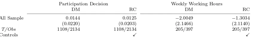
The probability to participate in the labor market (Participation Decision) and the number of working hours per week (Weekly Working Hours) are the two main outcomes analyzed. Participation decision is defined as to be doing any paid activity or to be seeking a job. Weekly working hours are the total reported hours of labor activity during a week. The former outcome is analyzed only for those who were reported as employed in the same activity since 2005. It was done in order to have a proxy of the effect on women who were working before the program full implementation. Otherwise, senior employees would be confused with new employees that were influenced in their participation decision by the program. As both groups face different decisions and restrictions that are relevant for this analysis, this restriction is necessary.

5 Data

We use the ECV2007 wich was designed for Bogot´a by the DANE and it is representative

bylocalidad in eachestrato. The survey has 26,585 household observations. Two household

questions of the survey are related to the program: the first, if household’s head knows the existence of the program (72.21%); the second, if at least one household member attended the program (1,275 households, 6.78% from those who positively answered the former question).

The dataset is restricted to women aged and over 15 who are household heads or his spouse. At the end, 22,939 households were considered (86.3%). 4 households we excluded due to the absence of educational information and 203 as a result of home ownership missing data. Another restriction was done: estratos 4, 5 and 6 were excluded as they are not beneficiaries of the program (35 treated households were excluded as a result). Therefore the final number of observations is 18,750 where 1,108 of them are treated units (87% of the original 1,275 beneficiary households). 494 of them were working and 9 were excluded as there no information about job seniority was provided. From these, 217 were working in the same activity before January 2005. In terms of individuals, those 1.108 households correspond to 4,565 individuals (relatives of the household-head), while the 217 households involves 904 individuals.

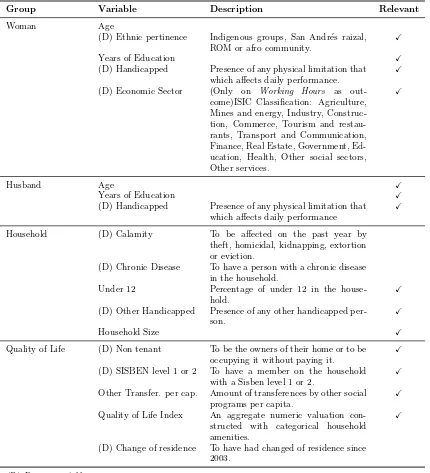
The selection of covariates set is probably the most crucial decision in a matching approach. According to Dehejia and Wahba (1999), results might be highly sensitive to the set of covariates. The covariates must be important for the outcome but also for explaining the propensity to be treated. Additionally, they must not be affected by the treatment status (Imbens, 2004).

(10)

on the appendix.

Most of these variables are relevant for labor participation decisions, but some of the usual were excluded 11_{. This is the case of the presence of other unemployed individuals}

and household income; those variables could be also explained by treatment status so they must be omitted. In the case of working hours, variables like economic sector wages were excluded due to the same reason.

As said, we analyze participation decision and working hours. For the working hours analysis the sample was restricted to women who had been working in the same occupation since January 2005. The idea is to analyze only women who had already a job before they entered to the program. Otherwise, information about women who decided to participate on the labor market due to the program could be introducing a bias on the estimations.

As we can see on figure 2(b), the quality of life index distributions of the treated and untreated groups overlap, there are no discontinuities. It also happens with the other continuous covariates as can be seen on figure 2. In particular, it seems that the program beneficiaries who are also receptors of other kind of programs transfers are not very different from the control group.

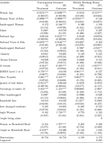
Covariates relevance was also checked. Table 2 resume the regressions of the treatment and the two outcomes against the covariates. The following covariates are not significant in any regression: calamity, chronic disease, change of residence and another handicapped presence. Specifications including and excluding those covariates will be taken into account. Household composition groups are defined depending on the marital status of the self-reported household head. This is done in order to take into account the presence of potential income earners that will share it with their household. Even though this criterion enables to split the sample in further groups than the marital status (for example, the presence of older children), the following classification was done in order to ensure the sample size for each one.

1. Single: Women who live alone

2. Couple: Women who live only with their spouse

3. Single-Head: Women who are the household head and do not live with their spouse

4. Couple-Head: Women who are either the household head or the spouse of the household head

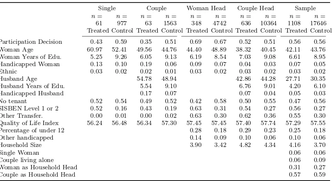
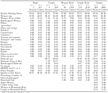
There is another important reason for differences in labor supply reaction: there are differences between the woman covariates within those groups as can be seen in tables 3 and 4.

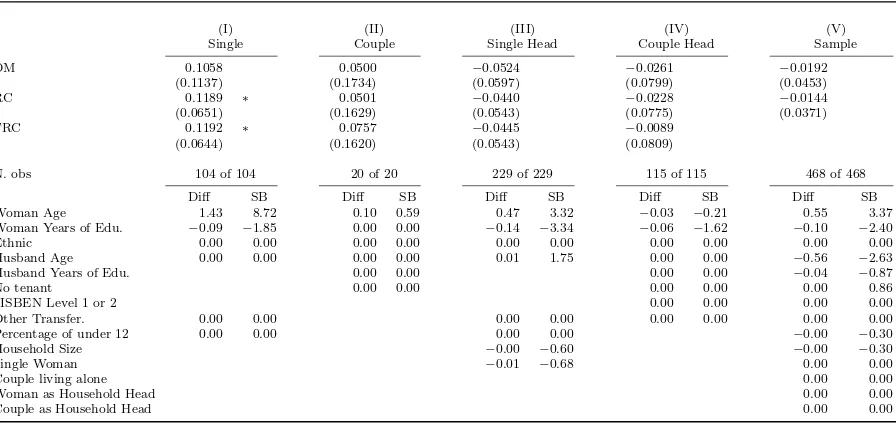
Before presenting the matching process results, tables 3 and 4 information must be complemented. Tables 5 and 6 present the differences between control and treated groups

(11)

per household group and the associated standardized bias. In all cases, there are significant differences in key variables like age and years of education. The matching procedure goal is to reduce them to insignificance. In that way, the treatment and control groups would be comparable.

6 Estimation

In this section we present the results of our estimations. First, we present results about the balance property of the matching procedure. Then we present the results about the effect of the program on female labor supply. Finally we present some robustness checks of our results.

6.1 Balance Property

The main objective of matching procedures is to ensure balance. Tables 5 and 6 present the differences for each covariate between control and treatment groups before and after matching. It includes the significance level for a difference of means test, the SB as defined by equation (3) and the SB percentage reduction. As can be seen, all differences in each household group are insignificant after applying the matching procedure.

A good illustration of matching quality is the density of the propensity score for control and treatment groups before and after the matching. Figure 1 shows those kernel densities by each outcome (as the working hours sample is a subset of the participation decision one and as it includes further controls). The densities for the matching for the specific household groups are presented on figures 3 and 4. In all cases the quality of the process can be seen: the propensity scores before matching are notoriously different but are very similar after it. Additionally, at first sight common support seems to be assured. In fact, using a caliper of 0.01, all treated observations are included for participation decision and 3 are lost in the weekly working hours’ specification. In both cases the balance property seems to be achieved in all variables as no significant mean difference remains. Moreover, most of the standardized bias are below 5%, as usual empirical studies (Caliendo and Kopeinig, 2005). Those results can be found in table 38 for participation decision and in table 43 for working hours. Along this paper, different variations of the matching procedure are implemented and presented. Their respective balance property tables are presented on the additional tables section on the appendix C.3.

6.2 Main results

(12)

covariates presented in section 5. Finally we allow the effect to differ in both household types and other covariates.

6.2.1 General results

Table 7 present the DM and RC estimators as defined by equations (4) and (5) for the ATT on the overall group. A positive effect on the participation decision and a negative one on working hours are presented. However, those effects are small and not significant.

What we are going to see is that the impact of the program is heterogeneous as it depends of the type of household analyzed. Heterogenous effects are found when the impact is measured in some specific households. Next, results are presented differencing by household composition groups, cohorts, family size, presence of children, years of education, change of residence, presence of other transferences and SISBEN level, and the type of work and seniority (only for working hours).

6.2.2 Household Composition

Table 8 presents the same results discriminating by household composition. It is just as the previous table but includes the FRC estimator as defined by equation (6). In this case, significant results at 10% level are found for the Couple-Head group, about 5 additional pp. The FRC estimator leads to a significant effect on Couple working hours. However, the Single and Couple groups’ effects are difficult to analyze as they involve a small number of treated observations: when they are included in the huge regression of FRC the variance structure changes enough for displaying this result.

6.2.3 Covariates Groups

Table 11 to 18 desegregate the overall effect into different individual and household covari-ates. Those results are presented in detail next.

(13)

Household composition variables are also relevant (see tables 12 and 16). Larger families drive to a notorious positive impact on participation decision: families with five or more members have 15 additional pp. The same pattern is not as clear for working hours’ decision: a positive impact is found for families with three members but it is not robust to the estimator. This can be understood in two ways: first, as a higher income is needed with larger families, additional consumption might be preferred to leisure; second, as there are more people available to work, women may concentrate on home related activities rather than on working. The presence of children has a different impact. The participation decision seems to be decreasing with a higher percentage of under-twelve, while a clear and huge negative impact on working hours is found for households with a higher number of small children: around 11 fewer working hours per week for families with small children are equal or more than 80%. In this case, household activities requires more attention so the time is not used in increasing the income but in childcare and similar activities.

(14)

6.2.4 Covariates within household groups

Our previous results show us the heterogeneous impact of the program when analyzing some characteristics. However, those effects are enhanced by the combination of some of those characteristics. Tables 19 to 26 explore the same covariates of the former tables but for the two bigger household composition groups. Results are mostly the same but more intense.

By cohorts (tables 19 and 23), the impact on Couple-Head women close to retirement age is huge: nearly 24 additional pp. For the Single-Head case, the impact on younger women is also noticeable: 14 fewer pp. But we also found an increment of 11 pp. for women in retirement age. Hence, it is not only a matter of being younger or older but the combination with the household composition.

By household covariates (tables 20 and 24), the impact follows as similar heterogeneous pattern. By household size, Single-Head impact is negative for smaller families and positive for the bigger. However, these results have a high variance. For Couple-Head, the two forces behind previously described are visible here: in a small household the impact could be even negative, but it becomes positive with a bigger household. However, for very big families, the impact is again negative. For children under 12 participation in the household, there is no clear pattern for Couple-Head but there is for Single-Head. Women living alone with small children are highly discouraged to work if they found additional income sources. However, if their household is big, they still need to work. In their cases, the relative size of the transfers is relevant for determining the impact of the program.

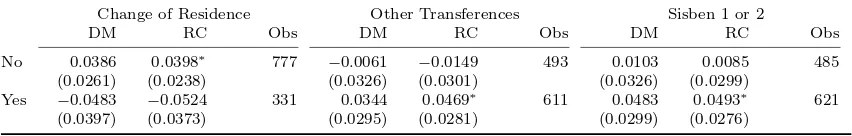
Finally, under the final set of covariates (tables 22 and 26), for Single-Head the impact does not change enough to be noticed. That is not the case of Couple-Head households. Women who live longer on the neighborhood and probably have a better social network, work more after being treated: the effect is positive and with small variance (significant at 5% level) while the impact could be negative for incoming women. The presence of other transferences enhances a little the impact.

6.3 Robustness Checks

Results are robust to matching methodology and to covariates specification. Two alterna-tive methodologies with similar results are presented. As mentioned, covariates specifica-tion is crucial and may drive to different coefficients. Our results stand this test.

(15)

estimator) while the sign becomes unclear for the working hours outcome. Specification 4 includes quality of life variables and the coefficients for CM and RC for the participation decision case fall to 6 pp. The FRC estimator falls to 4pp but is not significant even at 5% level. Again, the result for working hours is ambiguous. Finally, when selecting the relevant covariates as described on the identification strategy section, the coefficients for DM and RC fall to 5.5 pp. at 10% level and FRC keep on 4pp but it is still non-significant. For working hours, all three estimators drive positive bur remain unsignificant. From this exercise we can emphasise the relevance of the covariates groups:, household composition variables like household size and the presence of kids are relevant for the women response to the in-kind transfer.

Other matching methodologies were also tried in order to very the results. The coars-ened exact matching procedure (CEM) from Iacus et al. (2009) and the nearest neighbor matching across the variables from Abadie et al. (2004) results are presented in table 27 for the case of participation decision outcome . The CEM procedure, which garantees balanced outcomes, included only 225 observations from the 1108 available for the participation de-cision12. Abadie et al. (2004) procedure allows observations to be included more than once. The results are similiar in all methods, in particular for the Couple-Head result. For both PS Mahalanobis and the covariates matching, the estimators are significant at 10% significance level. The CEM estimate is close in terms of coefficient but is not significant, probably because of the small sample size involved in the method.

A final robustness check is done by including the ECV2003 data in order to use a placebo methodology to check the reliability of the matching methodology. That is, we checked if there were differences before the program start. As we do not have panel data, a “treatment”group was constructed using the most accurate matching methodology between 2003 and 2007 data. In order to implement this placebo test, two steps are required: first, to obtain the treatment group in 2003; second, to do the matching procedure in 2003. For the first step, the treatment group in ECV2007 was matched with ECV2003 data using the subset of covariates that are present in both datasets. As we need a treatment group as similar as possible, the CEM procedure was implemented. This matched subset in ECV2003 is now considered as the new treatment group for the matching “before” the program. In the second step, the same matching procedure used on the main results is applied to the 2003 data. Table 28 summarizes the first step: prematching and postmatching balance. As can be observed, the matching quality is good for the included covariates but half of the original ECV2007 treated observations were not matched. Table 29 presents the results of the second step. For the Single, there is a positive effect that is significant at 10% level. For all the other groups, the effect is not significant. Hence, our results are robust for groups other than Single13_.

12_{For the weely working hours outcome, only 17 observations were included in the CEM procedure. As}

a results, the summarizing table is not presented here.

13_{This test was also done using Mahalanobis Nearest Neighborhood Matching within the Calipers for}

(16)

7 Conclusions

Comedores Comunitarios attendees give us the opportunity to analyze an in-kind transfer

program effect on labor supply. Often, food and nutrition programs have negative effects on labor supply. However, in this case, both significant positive and negative effects were found depending on the type of householdt. We have shown that labor supply reacts in different ways to alternative combination of covariates that define different family patterns. If policy makers want to prevent distortions (or enhance some effects) of this type of programs, they should make emphasis in complementary programs for those particular kind of families. Hence, the program design must involve not only the food, but also promote access and attendance to other facilities like childcare, work training and education.

References

Abadie, A., Drukker, D., Herr, J. L. and Imbens, G. W. (2004). Implementing matching estimators for average treatment effects in stata,Stata Journal 4(3): 290–311.

Abadie, A. and Imbens, G. W. (2006). On the failure of the bootstrap for matching esti-mators,NBER Technical Working Papers 0325, National Bureau of Economic Research, Inc.

Altonji, J. G. and Blank, R. M. (1999). Race and gender in the labor market,inO. Ashen-felter and D. Card (eds), Handbook of Labor Economics, Vol. 3 of Handbook of Labor

Economics, Elsevier, chapter 48, pp. 3143–3259.

Arango, L. E. and Posada, C. E. (2007). Labor participation of married women in colombia,

Desarrollo y Sociedad.

Becker, G. S. (1973). A theory of marriage: Part i,Journal of Political Economy81(4): 813– 46.

Bingley, P. and Walker, I. (2008). The labor supply effect of in-kind transfers, Working

Papers 200820, Geary Institute, University College Dublin.

Blevins, J. and Khan, S. (2009). Distribution-Free Estimation of Heteroskedastic Binary Response Models in Stata. Second Version.

Bogotá Mayor (2007). La ciudad tendrá 54 comedores comunitarios más.

URL:http://www.bogota.gov.co/portel/libreria/php/frame detalle.php?h id=16559&patron=01.11

(17)

Caliendo, M. and Kopeinig, S. (2005). Some practical guidance for the implementation of propensity score matching, IZA Discussion Papers 1588, Institute for the Study of Labor (IZA).

Charry L., A. (2003). La participaci´on laboral de las mujeres no jefes de hogar en colom-bia y el efecto del servicio dom´estico, Technical Report 262, Banco de la Republica de Colombia.

Chiappori, P.-A. (1992). Collective labor supply and welfare,Journal of Political Economy 100(3): 437–67.

Cremer, H. and Gahvari, F. (1997). In-kind transfers, self-selection and optimal tax policy,

European Economic Review 41(1): 97 – 114.

Currie, J. and Gahvari, F. (2007). Transfers in cash and in kind: Theory meets the data,

NBER Working Papers 13557, National Bureau of Economic Research, Inc.

Dehejia, R. H. and Wahba, S. (1999). Causal effects in non-experimental studies: Re-evaluating the evaluation of training programs, Journal of the American Statistical

As-sociation 94(448): 1053–1062.

Fraker, T. and Moffitt, R. (1988). The effect of food stamps on labor supply : A bivariate selection model, Journal of Public Economics35(1): 25–56.

Gahvari, F. (1994). In-kind transfers, cash grants and labor supply, Journal of Public

Economics 55(3): 495–504.

Gamboa, L. F., Cortés, D. and Gonzáles, J. I. (2000). Algunas consideraciones anal´ıticas sobre el estándar de vida, Revista de Econom´ıa del Rosario .

Hagstrom, P. A. (1996). The food stamp participation and labor supply of married couples: An empirical analysis of joint decisions,Journal of Human Resources31(2): 383–403.

Hoynes, H. W. and Schanzenbach, D. (2007). Consumption responses to in-kind transfers: Evidence from the introduction of the food stamp program, NBER Working Papers

13025, National Bureau of Economic Research, Inc.

Iacus, S., King, G. and Porro, G. (2009). Causal inference without balance checking: Coarsened exact matching, Typescript, University of Milan, Harvard University, and

University of Trieste .

Imbens, G. W. (2004). Nonparametric estimation of average treatment effects under exo-geneity: A review,The Review of Economics and Statistics 86(1): 4–29.

(18)

Killingsworth, M. R. and Heckman, J. J. (1987). Female labor supply: A survey,Handbook

of Labor Economics, Vol. 1 ofHandbook of Labor Economics, Elsevier, chapter 2, pp. 103–

204.

Leonesio, M. V. (1988). In-kind transfers and work incentives,Journal of Labor Economics 6(4): 515–529.

Leuven, E. and Sianesi, B. (2003). Psmatch2: Stata module to perform full mahalanobis and propensity score matching, common support graphing, and covariate imbalance testing.

Meng, X. and Ryan, J. (2010). Does a food for education program affect school outcomes? the bangladesh case, Journal of Population Economics 23: 415–447. 10.1007/s00148-009-0240-0.

Moffitt, R. (2002). Welfare programs and labor supply, NBER Working Papers 9168, National Bureau of Economic Research, Inc.

Neary, J. P. and Roberts, K. W. S. (1980). The theory of household behaviour under rationing, European Economic Review13(1): 25 – 42.

Núñez, J. and Cuesta, L. (2007). ¿cómo va bogotá sin hambre?, DOCUMENTOS CEDE

003792, Universidad de Los Andes-CEDE. CEDE.

Posada, C. E. and Arango, L. E. (2003). La participaci´on laboral en colombia,Borradores

de economia, Banco de la Republica de Colombia.

Robbins, D. and Salinas, D. (2007). Partial equilibrium models of labor supply, Mimeo . Universidad de Antioquia.

Robbins, D., Salinas, D. and Manco, A. (2009). Female labor supply and its determinants: Evidence for colombia through estimates of synthetic cohorts, Lecturas de Econom´ıa 70: 137–163.

Rosenbaum, P. R. and Rubin, D. B. (1985). Constructing a control group using multivariate matched sampling methods that incorporate the propensity, The American Statistician 39(1): 33–38.

Rubin, D. B. (2006). Matched Sampling for Causal Effects, Cambridge University Press.

(19)

Skoufias, E. and Gonzalez-Cossio, T. (2008). The impacts of cash and in-kind transfers on consumption and labor supply: Experimental evidence from rural mexico, Policy

Research Working Paper Series 4778, The World Bank.

Smith, J. P. and Cogan, J. F. (1980). Female Labor Supply: Theory and Estimation, Princeton University Press.

Tenjo, J. and Ribero, R. (1998). Participaci´on, desempleo y mercados laborales en

(20)

(21)

A

Main Tables

[image:21.612.92.522.180.653.2]

A.1 Descriptive Information

Table 1: Covariates

Group Variable Description Relevant

Woman Age

(D) Ethnic pertinence Indigenous groups, San Andr´es raizal, ROM or afro community.

X

Years of Education X

(D) Handicapped Presence of any physical limitation that which affects daily performance.

X

(D) Economic Sector (Only on Working Hours as out-come)ISIC Classification: Agriculture, Mines and energy, Industry, Construc-tion, Commerce, Tourism and restau-rants, Transport and Communication, Finance, Real Estate, Government, Ed-ucation, Health, Other social sectors, Other services.

X

Husband Age X

Years of Education X

(D) Handicapped Presence of any physical limitation that which affects daily performance

X

Household (D) Calamity To be affected on the past year by theft, homicidal, kidnapping, extortion or eviction.

(D) Chronic Disease To have a person with a chronic disease in the household.

Under 12 Percentage of under 12 in the house-hold.

X

(D) Other Handicapped Presence of any other handicapped per-son.

X

Household Size X

Quality of Life (D) Non tenant To be the owners of their home or to be occupying it without paying it.

X

(D) SISBEN level 1 or 2 To have a member on the household with a Sisben level 1 or 2.

X

Other Transfer. per cap. Amount of transferences by other social programs per capita.

X

Quality of Life Index An aggregate numeric valuation con-structed with categorical household amenities.

X

(D) Change of residence To have had changed of residence since 2003.

(22)

(23)

[image:23.612.138.471.123.585.2]

Table 2: Covariates relevance

Variables Participation Decision Weekly Working Hours

(I) (II) (III) (IV)

Treatment Outcome Treatment Outcome

Woman Age -0.0154*** -0.0496*** -0.0133 -0.133***

(0.00357) (0.00196) (0.0100) (0.0404)

Woman Years of Edu. -0.0996*** 0.0999*** -0.0788*** -0.138

(0.0100) (0.00481) (0.0231) (0.0875)

Handicapped Woman 0.172 -0.348*** 0.390 -1.550

(0.133) (0.0799) (0.331) (2.021)

Ethnic 0.360* -0.0759 0.271 0.107

(0.206) (0.125) (0.486) (2.027)

Husband Age 0.00124 0.0127*** 0.0149 0.00784

(0.00394) (0.00206) (0.0109) (0.0424)

Husband Years of Edu. -0.0476*** 0.0140*** -0.0482* -0.162

(0.0120) (0.00531) (0.0276) (0.0991)

Handicapped Husband 0.273* 0.128 0.596* -4.945**

(0.162) (0.0943) (0.346) (2.124)

Calamity 0.0911 0.0285 0.149 0.125

(0.0913) (0.0516) (0.209) (0.931)

Chronic Disease 0.0509 -0.0588 0.0469 0.515

(0.0724) (0.0371) (0.166) (0.646)

No tenant -0.164** -0.203*** -0.215 -1.825***

(0.0723) (0.0364) (0.162) (0.611)

SISBEN Level 1 or 2 0.770*** -0.0156 0.901*** -0.727

(0.0677) (0.0380) (0.165) (0.796)

Other Transfer. 0.681*** 0.433*** 0.862*** 0.241

(0.0762) (0.0400) (0.176) (0.685)

Quality of Life Index -0.0153** 0.00448 -0.0276 -0.0555

(0.00758) (0.00562) (0.0177) (0.117)

Percentage of under 12 0.833*** -1.453*** 0.000885 -2.983*

(0.202) (0.109) (0.458) (1.713)

Other handicapped 0.206* -0.0646 -0.0986 -0.628

(0.115) (0.0683) (0.286) (1.433)

Household Size 0.0314 0.0192 0.122** -0.0301

(0.0230) (0.0135) (0.0510) (0.257)

Have changed residence 0.101 0.0303 -0.282 -0.553

(0.0750) (0.0404) (0.191) (0.688)

Single Woman 0.341 1.716*** 0.770 -1.523

(0.307) (0.161) (0.841) (2.927)

Couple living alone 0

Woman as Household Head -0.351 1.977*** 0.402 0.160

(0.275) (0.140) (0.734) (2.630)

Couple as Household Head -0.339** 0.0386 -0.148 1.018

(0.156) (0.0691) (0.416) (1.316)

Observations 18.754 18.754 4.150 4.172

R-squared 0.045

Robust standard errors in parentheses for IV. ***p<0.001 **p<0.05 *p<0.1 Economic sector not reported but they are included on columns 3 and 4 I, II and III are logistic regressions. IV is an OLS regression.

(24)

[image:24.612.138.478.121.307.2]

Table 3: Descriptive Statistics for Participation Decision

Single Couple Woman Head Couple Head Sample n=

61 n=

977 n=

63 n= 1563

n= 348

n= 4742

n= 636

n= 10364

n= 1108

n= 17646 Treated Control Treated Control Treated Control Treated Control Treated Control

Participation Decision 0.43 0.59 0.35 0.51 0.69 0.67 0.52 0.51 0.56 0.56 Woman Age 60.97 52.41 49.56 44.76 44.40 48.89 38.32 40.45 42.11 43.76 Woman Years of Edu. 5.25 9.26 6.05 9.13 6.19 8.54 7.03 9.08 6.61 8.95 Handicapped Woman 0.13 0.10 0.19 0.06 0.09 0.07 0.04 0.03 0.07 0.05 Ethnic 0.03 0.02 0.02 0.01 0.03 0.02 0.03 0.02 0.03 0.02 Husband Age 54.78 48.94 42.86 44.28 27.71 30.35 Husband Years of Edu. 5.54 9.10 6.76 9.01 4.20 6.10 Handicapped Husband 0.17 0.07 0.07 0.04 0.05 0.03 No tenant 0.52 0.54 0.49 0.52 0.42 0.58 0.50 0.55 0.47 0.56 SISBEN Level 1 or 2 0.52 0.16 0.43 0.19 0.63 0.31 0.54 0.27 0.56 0.27 Other Transfer. 0.00 0.01 0.00 0.02 0.63 0.30 0.62 0.36 0.55 0.30 Quality of Life Index 56.24 56.48 56.34 57.30 57.45 57.45 57.40 57.74 57.29 57.55 Percentage of under 12 0.28 0.18 0.29 0.23 0.25 0.18 Other handicapped 0.14 0.09 0.10 0.06 0.10 0.06 Household Size 3.90 3.42 4.82 4.34 4.16 3.70

Single Woman 0.06 0.06

Couple living alone 0.06 0.09

Woman as Household Head 0.31 0.27

Couple as Household Head 0.57 0.59

***p<0.001 **p<0.05 *p<0.1

(25)

[image:25.612.134.479.121.417.2]

Table 4: Descriptive Statistics for Weekly Working Hours

Single Couple Woman Head Couple Head Sample n= 7 n= 217 n= 8 n= 283 n= 83 n= 1354 n= 110 n= 2110 n= 208 n= 3964 Treated Control Treated Control Treated Control Treated Control Treated Control

Weekly Working Hours 38.12 48.33 42.71 47.90 47.99 48.53 47.75 48.04 47.32 48.20 Woman Age 47.59 42.05 40.35 36.36 40.07 42.16 38.69 38.06 39.61 39.46 Woman Years of Edu. 6.35 11.34 7.53 11.41 6.71 9.62 7.63 10.12 7.22 10.14 Handicapped Woman 0.00 0.05 0.12 0.02 0.09 0.03 0.03 0.02 0.05 0.02 Ethnic 0.12 0.02 0.00 0.02 0.02 0.01 0.02 0.02 0.03 0.02 Agriculture 0.00 0.00 0.00 0.01 0.01 0.01 0.00 0.01 0.00 0.01 Mines and energy 0.00 0.00 0.00 0.00 0.00 0.00 0.00 0.00 0.00 0.00 Industry 0.29 0.13 0.29 0.11 0.13 0.16 0.18 0.19 0.17 0.17 Construction 0.00 0.01 0.00 0.02 0.01 0.01 0.00 0.01 0.00 0.01 Commerce 0.29 0.21 0.29 0.25 0.27 0.21 0.24 0.21 0.25 0.21 Tourism and restrnts. 0.12 0.08 0.12 0.07 0.06 0.10 0.09 0.08 0.08 0.09 Transport and Comm. 0.06 0.05 0.00 0.05 0.02 0.04 0.02 0.04 0.02 0.04 Finance 0.06 0.02 0.00 0.03 0.01 0.02 0.01 0.02 0.01 0.02 Real Estate 0.00 0.13 0.12 0.10 0.09 0.11 0.09 0.09 0.09 0.10 Government 0.06 0.07 0.00 0.04 0.02 0.04 0.02 0.04 0.02 0.04 Education 0.00 0.09 0.06 0.09 0.04 0.06 0.04 0.06 0.04 0.06 Health 0.06 0.07 0.00 0.08 0.08 0.06 0.09 0.08 0.08 0.07 Other social sector 0.00 0.06 0.00 0.06 0.04 0.06 0.05 0.05 0.04 0.05 Other services 0.06 0.06 0.12 0.06 0.22 0.10 0.14 0.09 0.17 0.09 Husband Age 46.71 40.62 43.20 41.69 24.81 25.88 Husband Years of Edu. 7.47 10.77 7.08 9.70 4.06 6.13 Handicapped Husband 0.18 0.04 0.07 0.03 0.04 0.02 No tenant 0.65 0.38 0.29 0.39 0.32 0.47 0.49 0.52 0.42 0.48 SISBEN Level 1 or 2 0.24 0.14 0.47 0.16 0.61 0.30 0.52 0.24 0.54 0.25 Other Transfer. 0.00 0.01 0.00 0.02 0.71 0.35 0.65 0.38 0.63 0.32 Quality of Life Index 56.57 56.48 56.45 57.43 57.79 57.49 57.24 57.76 57.40 57.57 Percentage of under 12 0.32 0.20 0.26 0.23 0.26 0.19 Other handicapped 0.11 0.07 0.08 0.05 0.09 0.05 Household Size 3.98 3.31 4.81 4.25 4.25 3.58

Single Woman 0.04 0.06

Couple living alone 0.04 0.08

Woman as Household Head 0.39 0.32

Couple as Household Head 0.54 0.54

***p<0.001 **p<0.05 *p<0.1

(26)

[image:26.612.116.733.79.206.2]

Table 5: Balance Status for Participation Decision

Single Couple Single Couple Couple Head

Before After BR Before After BR Before After BR Before After BR Diff SB Diff SB Diff SB Diff SB Diff SB Diff SB Diff SB Diff SB Woman Age 8.55∗ ∗∗ 46.16 −0.28 −1.50 96.74 4.79∗ ∗ 27.78 −1.25 −7.27 73.83 −4.49∗ ∗∗ −31.39 0.62 4.33 86.21 −1.65∗ ∗∗ −11.45 0.47 3.99 77.69 Woman Years of Edu. −4.01∗ ∗∗ −76.17 0.02 0.31 99.59 −3.08∗ ∗∗ −65.06 0.24 5.01 92.30 −2.35∗ ∗∗ −55.30 −0.16 −3.66 93.37 −2.34∗ ∗∗ −55.83 −0.01 −0.36 99.31 Handicapped Woman 0.03 8.27 0.00 0.00 100.00 0.13∗ ∗∗ 40.92 −0.03 −10.44 74.49 0.02 8.12 0.01 3.17 60.97 0.02∗ ∗∗ 8.98 0.00 2.50 38.65 Ethnic 0.01 4.90 0.02 9.78 −99.39 0.00 0.94 0.00 0.00 100.00 0.01 6.70 0.00 2.01 70.06 0.01∗ ∗ 7.01 0.01 4.38 44.30 Husband Age 5.84∗ ∗ 33.26 −0.51 −2.90 91.29 −2.63∗ ∗∗ −10.99 0.66 4.99 53.64 Husband Years of Edu. −3.56∗ ∗∗ −78.74 −0.10 −2.25 97.14 −1.90∗ ∗∗ −37.84 −0.15 −3.74 93.22 Handicapped Husband 0.10∗ ∗∗ 30.84 0.02 5.17 83.22 0.02∗ ∗∗ 8.08 0.00 1.38 86.16 No tenant −0.01 −2.55 −0.02 −3.27 −28.38 −0.03 −5.34 −0.02 −3.38 36.78 −0.16∗ ∗∗ −32.37 0.00 0.58 98.20 −0.08∗ ∗∗ −16.37 −0.01 −2.52 76.89 SISBEN Level 1 or 2 0.36∗ ∗∗ 82.25 0.00 0.00 100.00 0.24∗ ∗∗ 53.15 0.03 7.55 85.79 0.32∗ ∗∗ 66.77 0.00 0.00 100.00 0.29∗ ∗∗ 61.54 0.00 0.00 100.00 Other Transfer. −0.01 −16.41 0.00 0.00 100.00 −0.02 −17.65 0.00 0.00 100.00 0.33∗ ∗∗ 70.59 −0.01 −2.45 96.53 0.26∗ ∗∗ 54.08 −0.01 −1.95 96.32 Quality of Life Index −0.25 −9.04 −0.25 −9.36 −3.60 −0.96∗ ∗∗ −39.30 −0.25 −10.22 74.00 −0.00 −0.05 −0.01 −0.25 −370.00 −0.26∗ ∗∗ −6.31 −0.01 −0.13 98.12 Percentage of under 12 0.11∗ ∗∗ 47.22 0.01 2.73 94.22 0.07∗ ∗∗ 34.40 1.22 95.96 Other handicapped 0.04∗ ∗∗ 14.05 0.01 2.74 80.52 0.04∗ ∗∗ 13.70 0.00 1.16 90.90 Household Size 0.48∗ ∗∗ 28.89 0.22∗ 13.45 53.43 0.46∗ ∗∗ 26.33 0.12 8.26 74.88

***p<0.001 **p<0.05 *p<0.1

Source:Own calculations

Table 6: Balance Status for Weekly Working Hours

Single Couple Single Couple Couple Head

Before After BR Before After BR Before After BR Before After BR Diff SB Diff SB Diff SB Diff SB Diff SB Diff SB Diff SB Diff SB

Woman Age 8.55∗ ∗∗ 46.16 −1.80 −10.81 84.89 4.79∗ ∗ 27.78 3.60 27.38 −14.73 −4.49∗ ∗∗ −31.39 1.01 10.00 37.12 −1.65∗ ∗∗ −11.45 −0.72 −7.99 54.26 Woman Years of Edu. −4.01∗ ∗∗ −76.17 −1.60 −28.12 68.38 −3.08∗ ∗∗ −65.06 −1.00 −19.46 72.26 −2.35∗ ∗∗ −55.30 0.09 2.02 97.15 −2.34∗ ∗∗ −55.83 0.25 5.74 90.33 Handicapped Woman 0.03 8.27 0.00 0.00 100.00 0.13∗ ∗∗ 40.92 0.00 0.00 100.00 0.02 8.12 0.03 11.00 57.26 0.02∗ ∗∗ 8.98 −0.02 −10.52 17.83 Ethnic 0.01 4.90 0.00 0.00 100.00 0.00 0.94 0.00 0.00 100.00 0.01 6.70 0.01 8.56 −160.00 0.01∗ ∗ 7.01 0.01 6.52 14.65 Agriculture −0.00 −6.40 0.00 0.00 100.00 −0.00 −8.01 0.00 0.00 100.00 −0.00 −2.58 0.00 0.00 100.00 −0.00 −2.55 0.01 10.60 −380.00 Mines and energy −0.00 −4.52 0.00 0.00 100.00 −0.00 −3.58 0.00 −0.00 −4.11 0.00 −0.00 −3.53 0.00 0.00 100.00 Industry 0.02 7.93 0.20 48.73 −14.21 0.03 13.40 0.20 58.17 −9000.00 −0.01 −4.81 −0.03 −7.06 9.86 −0.00 −1.53 −0.04 −10.03 4.20 Construction −0.00 −9.06 0.00 −0.01 −11.90 0.00 0.00 100.00 0.00 2.50 0.00 0.00 100.00 −0.00 −3.22 0.00 0.00 100.00 Commerce −0.02 −7.02 0.00 0.00 100.00 −0.02 −7.77 0.00 0.00 100.00 0.03∗ ∗ 10.44 −0.06 −13.84 54.35 0.02∗ 5.27 −0.03 −6.43 62.36 Tourism and restrnts. −0.01 −3.80 0.00 0.00 100.00 0.00 1.72 0.00 0.00 100.00 −0.01 −6.18 0.01 6.08 69.43 −0.00 −1.05 0.01 4.30 22.98 Transport and Comm. −0.01 −4.42 0.00 0.00 100.00 −0.02 −21.40 0.00 0.00 100.00 −0.01 −5.96 0.00 0.00 100.00 −0.01∗ ∗ −6.90 0.02 12.03 −27.04 Finance 0.01 6.36 0.00 0.00 100.00 −0.01 −15.26 0.00 0.00 100.00 −0.01 −11.32 0.00 0.00 100.00 −0.01∗ ∗ −8.43 0.00 0.00 100.00 Real Estate −0.06∗ ∗ −36.16 0.00 0.00 100.00 −0.01 −3.60 −0.20 −63.26 −360.00 −0.01 −4.78 −0.01 −3.98 −230.00 −0.01 −3.62 0.02 7.11 −110.00 Government −0.01 −9.42 −0.20 −58.42 −380.00 −0.02 −18.39 0.00 0.00 100.00 −0.01 −6.26 0.00 0.00 100.00 −0.01∗ ∗ −8.23 0.00 0.00 100.00 Education −0.04 −28.82 0.00 0.00 100.00 −0.02 −11.90 0.00 0.00 100.00 −0.01 −6.29 0.03 10.61 −17.75 −0.01∗ ∗ −8.93 0.01 3.70 36.66 Health −0.01 −9.42 0.00 0.00 100.00 −0.03 −25.96 0.00 0.00 100.00 0.01 5.45 0.03 10.34 −660.00 0.00 1.87 0.01 3.68 42.13 Other social sector −0.03 −24.72 0.00 0.00 100.00 −0.02 −22.32 0.00 0.00 100.00 −0.01 −8.42 0.03 11.69 −5.58 −0.00 −2.70 0.02 7.17 70.27 Other services −0.01 −8.84 0.00 0.00 100.00 0.01 4.90 0.00 0.00 100.00 0.06∗ ∗∗ 22.91 0.01 3.76 84.67 0.03∗ ∗∗ 14.75 −0.03 −9.38 40.04 Husband Age 5.84∗ ∗ 33.26 −2.20 −14.31 50.05 −2.63∗ ∗∗ −10.99 −0.54 −4.95 81.71 Husband Years of Edu. −3.56∗ ∗∗ −78.74 0.40 8.28 85.68 −1.90∗ ∗∗ −37.84 0.06 1.37 98.12 Handicapped Husband 0.10∗ ∗∗ 30.84 0.00 0.00 100.00 0.02∗ ∗∗ 8.08 −0.02 −7.22 77.08 No tenant −0.01 −2.55 0.00 0.00 100.00 −0.03 −5.34 0.00 0.00 100.00 −0.16∗ ∗∗ −32.37 0.09 17.83 53.10 −0.08∗ ∗∗ −16.37 −0.03 −5.83 −210.00 SISBEN Level 1 or 2 0.36∗ ∗∗ 82.25 0.20 56.70 −770.00 0.24∗ ∗∗ 53.15 0.00 0.00 100.00 0.32∗ ∗∗ 66.77 0.01 2.68 96.45 0.29∗ ∗∗ 61.54 −0.03 −6.24 91.56 Other Transfer. −0.01 −16.41 0.00 0.00 100.00 −0.02 −17.65 0.00 0.00 100.00 0.33∗ ∗∗ 70.59 −0.04 −8.08 90.09 0.26∗ ∗∗ 54.08 0.06 11.83 78.08 Quality of Life Index 0.25 9.04 0.19 10.28 83.46 0.96 39.30 0.92 61.41 11.50 0.00 0.05 0.38 18.82 51.20 0.26 6.31 0.44 8.17 61.88

[image:26.612.119.757.275.494.2]

(27)

[image:27.612.95.518.160.226.2]

A.2 Estimation Outputs

Table 7: Full Sample

Participation Decision Weekly Working Hours

DM RC DM RC

All Sample 0.0144 0.0125 −2.0049 −1.3034

(0.0220) (0.0203) (2.1466) (2.1140)

T/Obs 1108/2134 1108/2134 205/397 205/397

Controls X X

Robust standard errors in parentheses for RC and FRC. ***p<0.001 **p<0.05 *p<0.1

DM:Difference of means. RC:Regression within each group.

Tr: Included treated observations. Obs: Total included observations. Source: Own calculations

Table 8: Main Results by Household Composition

Participation Decision Weekly Working Hours

DM RC FRC DM RC FRC

Single −0.0328 −0.0523 −0.0368 −15.4000 −18.3533 −15.7412

(0.0921) (0.0791) (0.0838) (9.9025) (0.0000) (9.9385)

Tr/Obs 61/120 61/120 1102/2123 5/10 5/10 192/369

Couple −0.0339 −0.0751 −0.0506 −6.0000 4.4629 −6.1774

(0.0907) (0.0786) (0.0789) (10.4642) (0.0000) (9.2504)

Tr/Obs 59/117 59/117 1102/2123 5/10 5/10 192/369

Single-Head −0.0376 −0.0233 −0.0282 −2.8250 −2.4755 −2.4919

(0.0365) (0.0306) (0.0313) (3.2900) (3.3345) (3.2185)

Tr/Obs 346/654 346/654 1102/2123 80/154 80/154 192/369

Couple-Head 0.0566∗ 0.0566∗ ∗ 0.0580∗ 2.4190 2.9701 2.7323

(0.0289) (0.0283) (0.0286) (3.2284) (3.3009) (3.2451)

Tr/Obs 636/1232 636/1232 1102/2123 105/198 105/198 192/369

Controls X X X X

DM:Difference of means. RC:Regression within each group. FRC:Regression using the full matched sample.

[image:27.612.92.519.349.527.2]

(28)

[image:28.612.66.764.80.212.2]

Table 9: Full Sample Matching Results for Participation Decision

Spe1. Spe2. Spe3. Spe4. Final

DM RC FRC DM RC FRC DM RC FRC DM RC FRC DM RC FRC Single 0.0000 −0.0020 −0.0009 0.0000 −0.0020 −0.0013 −0.0164 −0.0254 −0.0243 −0.0492 −0.0310 −0.0309 −0.0328 −0.0523 −0.0368

(0.0926) (0.0806) (0.0820) (0.0926) (0.0806) (0.0815) (0.0942) (0.0834) (0.0846) (0.0952) (0.0868) (0.0844) (0.0921) (0.0791) (0.0838) Couple −0.1111 −0.1096 −0.1097 0.0161 0.0193 0.0134 −0.1111 −0.1311 −0.1257 −0.0645 −0.0916 −0.0846 −0.0339 −0.0751 −0.0506

(0.0905) (0.0822) (0.0829) (0.0888) (0.0748) (0.0763) (0.0903) (0.0794) (0.0789) (0.0891) (0.0773) (0.0770) (0.0907) (0.0786) (0.0789) Single-Head −0.0461 −0.0455 −0.0456 −0.0461 −0.0455 −0.0456 −0.0029 −0.0048 −0.0054 0.0029 0.0075 0.0059 −0.0376 −0.0233 −0.0282

(0.0417) (0.0371) (0.0374) (0.0417) (0.0371) (0.0371) (0.0363) (0.0335) (0.0338) (0.0364) (0.0317) (0.0322) (0.0365) (0.0306) (0.0313) Couple-Head 0.0772∗ ₀_.₀₇₇₄∗ ₀_.₀₇₇₆∗ ₀_.₀₂₃₆ ₀_.₀₂₅₁ ₀_.₀₂₅₂ ₀_.₀₇₇₂∗∗∗ ₀_.₀₈₀₀∗∗∗ ₀_.₀₈₁₈∗∗∗ ₀_.₀₆₄₅∗∗ ₀_.₀₆₆₃∗∗ ₀_.₀₆₂₆∗∗ ₀_.₀₅₆₆∗ ₀_.₀₅₆₆∗∗ ₀_.₀₅₈₀∗

(0.0397) (0.0397) (0.0402) (0.0288) (0.0284) (0.0287) (0.0287) (0.0282) (0.0285) (0.0291) (0.0285) (0.0287) (0.0289) (0.0283) (0.0286)

Woman X X X X X X X X X X X X X X X

Husband X X X X X X X X X X X

Household Comp. X X X X X X X X X

Quality of Life X X X X X X

DM:Difference of means.RC:Regression within each group.FRC:Regression using the full matched sample.

Source: Own calculations

Table 10: Full Sample Matching Results for Weekly Working Hours

Spe1. Spe2. Spe3. Spe4. Final

DM RC FRC DM RC FRC DM RC FRC DM RC FRC DM RC FRC Single 3.0000 −0.2115 −4.9215 3.0000 −0.2115 −4.9527 −6.7500 −23.7660 −17.5786 −23.5000 −40.3866 −23.1368∗ ₋₁₅_.₄₀₀₀ ₋₁₈_.₃₅₃₃ ₋₁₅_.₇₄₁₂

(12.5019) (21.0992) (11.9448) (12.5019) (21.0992) (12.9058) (13.9007) (0.0000) (10.5207) (11.9704) (0.0000) (11.5222) (9.9025) (0.0000) (9.9385) Couple −25.5714 −21.9957 −23.5410∗∗−14.0000 −1.9421 −14.4831 −0.4000 −0.7573 2.3532 −31.3333 0.0000 −28.1106∗∗ −6.0000 4.4629 −6.1774

(9.8025) (12.3070) (8.4103) (10.2372) (12.8146) (9.6528) (10.1272) (14.7648) (9.5409) (13.5483) (0.0000) (10.9718) (10.4642) (0.0000) (9.2504) Single-Head −2.5122 −2.2593 −2.3388 −2.5122 −2.2593 −2.2021 −1.6049 −2.1932 −1.6410 −1.0000 −1.9146 −1.5984 −2.8250 −2.4755 −2.4919

(2.8253) (2.8037) (2.8074) (2.8253) (2.8037) (2.8087) (3.1353) (3.6370) (3.5978) (3.1644) (3.3286) (3.2603) (3.2900) (3.3345) (3.2185) Couple-Head 1.6789 1.5798 1.5464 0.4312 0.3205 0.3663 −1.9000 −0.7142 −1.3695 1.6422 2.2059 2.0007 2.4190 2.9701 2.7323

(2.9092) (2.9302) (2.9207) (2.8283) (2.7855) (2.7624) (3.0220) (3.0836) (3.0031) (3.0722) (3.0923) (2.9749) (3.2284) (3.3009) (3.2451)

Woman X X X X X X X X X X X X X X X

Husband X X X X X X X X X X X

Household Comp. X X X X X X X X X

Quality of Life X X X X X X

DM:Difference of means.RC:Regression within each group.FRC:Regression using the full matched sample.

[image:28.612.62.753.291.423.2]

(29)

A.3 Analysis by covariates

[image:29.612.97.526.598.692.2]

A.3.1 Participation Decision

Table 11: Overall effect on Participation Decision by Cohorts

Couple-Head

Age DM RC Obs

15-27 −0.0947∗ −0.0899∗ 169

(0.0564) (0.0528)

27-32 −0.0360 −0.0416 139

(0.0599) (0.0538)

32-37 0.0800 0.0747 150

(0.0566) (0.0540)

37-41 0.0000 −0.0126 137

(0.0603) (0.0580)

41-47 0.0000 0.0145 161

(0.0548) (0.0519)

47-55 0.1172∗∗ _0.1322∗∗ ₁₄₅

(0.0588) (0.0570)

55-97 0.0553 0.0644 199

(0.0441) (0.0406)

All Cohorts 0.014 0.013 1108

(0.022) (0.020)

11 observations were lost due to common support.

Table 12: Overall effect on Participation Decision by Household Covariates

Household Size Under 12

2 −0.023 −0.023 132 0.0−33.3 0.040 0.035 375

(0.063) (0.051) (0.037) (0.033)

3 −0.043 −0.041 231 33.3−50.0 0.012 0.018 400

(0.047) (0.043) (0.036) (0.034)

4 0.039 0.038 256 50.0−83.3 0.013 0.025 227

(0.045) (0.042) (0.049) (0.046)

5+ 0.142∗∗∗ _0.149∗∗∗ ₁₉₇ _83.3₋_. ₋_0.051 _0.007 ₉₈

(0.052) (0.049) (0.077) (0.061)

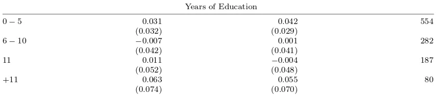
Table 13: Overall effect on Participation Decision by Work-Related Covariates

Years of Education

0−5 0.031 0.042 554

(0.032) (0.029)

6−10 −0.007 0.001 282

(0.042) (0.041)

11 0.011 −0.004 187

(0.052) (0.048)

+11 0.063 0.055 80

(0.074) (0.070)

(30)

Table 14: Overall effect on Participation Decision by Other Covariates

Change of Residence Other Transferences Sisben 1 or 2

DM RC Obs DM RC Obs DM RC Obs

No 0.0386 0.0398∗ ₇₇₇

−0.0061 −0.0149 493 0.0103 0.0085 485

(0.0261) (0.0238) (0.0326) (0.0301) (0.0326) (0.0299)

Yes −0.0483 −0.0524 331 0.0344 0.0469∗ 611 0.0483 0.0493∗ 621

(0.0397) (0.0373) (0.0295) (0.0281) (0.0299) (0.0276)

A.3.2 Working Hours

Table 15: Overall effect on Weekly Working Hours by Cohorts

Couple-Head

Age DM RC Obs

17-35 0.5319 2.0147 47

(4.4184) (4.7485)

35-41 −2.9730 −0.3189 37

(4.6160) (5.4299)

41-46.5 3.2821 4.9099 39

(5.2584) (5.9690)

46.5-55 −2.8000 0.2554 50

(4.0745) (4.4905)

55-89 −4.9474 −3.3710 19

(7.2038) (12.1949)

All Cohorts −2.005 −1.303 205

(2.147) (2.114)

[image:30.612.99.525.88.156.2]

Table 16: Overall effect on Weekly Working Hours by Household Covariates

2 −6.294 −8.659 17 0.0−25.0 0.744 1.121 82

(6.100) (5.115) (3.263) (3.319)

3 3.489 8.478∗ ₄₅ _25.0

−40.0 0.756 0.390 45

(4.057) (4.326) (5.005) (5.181)

4 −6.556 −6.921 45 40.0−80.0 −3.947 −1.370 38

(4.258) (4.671) (5.359) (5.898)

5+ 1.136 1.651 81 80.0−. −11.333∗∗ ₋_14.860∗∗ ₃₀

(3.487) (3.660) (4.729) (5.883)

(31)

Table 17: Overall effect on Weekly Working Hours by Work-Related Covariates

Years of Education Seniority

0−5 −4.229 −4.606 96 31-49 −3.460 −3.448 50

(3.367) (3.706) (4.278) (4.862)

6−10 −2.610 −3.520 41 49-96 −2.411 −2.416 56

(5.244) (5.407) (4.540) (5.100)

11 4.243 2.494 37 96-153 0.295 2.414 44

(4.034) (4.987) (4.331) (4.907)

+11 −3.333 −2.907 24 153-720 0.902 0.869 51

(5.292) (5.422) (4.128) (5.065)

Table 18: Overall effect on Weekly Working Hours by Other Covariates

Change of Residence Other Transferences Sisben 1 or 2 Wage Earner

DM RC Obs DM RC Obs DM RC Obs DM RC Obs

No −1.1728 −0.0596 162 0.2530 1.1293 83 −3.3750 −3.6371 88 −7.9211∗−8.5929∗ 76

(2.5778) (2.5171) (2.7876) (2.9305) (3.1323) (3.2376) (4.4726) (4.4770)

Yes 0.6667 −2.9460 39 −3.1967 −2.5188 122 −3.2069 −2.1378 116 0.0000 0.0377 119

(4.7423) (5.6300) (2.9850) (3.2348) (3.0393) (2.8673) (2.2518) (2.2233)

A.3.3 Participation Decision for Single-Head

Table 19: Effect on Participation Decision for Single-Head by Cohorts

Couple-Head

Age DM RC Obs

15-29 −0.1458∗ −0.1437 48

(0.0791) (0.0993)

29-35 0.0889 0.1044 45

(0.0718) (0.0764)

35-40 0.0000 0.0013 54

(0.0634) (0.0736)

40-44 −0.0789 −0.0906 38

(0.0802) (0.0781)

44-49 −0.0952 −0.0789 42

(0.0906) (0.0927)

49-55 0.0455 0.0884 44

(0.1069) (0.1060)

55-97 0.1111 0.1174∗ ₆₃

(0.0729) (0.0662)

All Cohorts −0.038 −0.023 346

(0.036) (0.031)

(32)

Table 20: Effect on Participation Decision for Single-Head by Household Covariates

3 −0.100 −0.100 70 0.0−33.3 0.017 −0.007 115

(0.084) (0.064) (0.067) (0.054)

4 −0.049 −0.045 102 33.3−50.0 −0.027 −0.013 111

(0.067) (0.057) (0.061) (0.050)

5 −0.057 −0.028 70 50.0−83.3 −0.157∗∗ ₋_0.130∗ ₇₀

(0.072) (0.065) (0.076) (0.069)

6+ 0.102 0.084 49 83.3−. −0.087 −0.077 46

(0.102) (0.080) (0.096) (0.089)

Table 21: Effect on Participation Decision for Single-Head by Work-Related Covariates

Years of Education

0−5 −0.026 0.002 193

(0.053) (0.042)

6−10 −0.049 −0.032 81

(0.065) (0.062)

11 −0.070 −0.069 43

(0.075) (0.071)

+11 0.000 0.021 27

(0.101) (0.098)

Table 22: Effect on Participation Decision for Single-Head by Other Covariates

Change of Residence Other Transferences Sisben 1 or 2

DM RC Obs DM RC Obs DM RC Obs

No −0.0290 −0.0188 241 −0.0079 −0.0140 127 −0.0313 −0.0020 128

(0.0447) (0.0372) (0.0646) (0.0570) (0.0580) (0.0482)

Yes −0.0577 −0.0724 104 −0.0461 −0.0390 217 −0.0688 −0.0559 218

(0.0620) (0.0624) (0.0428) (0.0362) (0.0466) (0.0391)