In this work we distinguish mainly three parts. In the first one we study some questions related to the stability of homographic solutions of the Planar Three Body Problem with some homogeneous potential. As we are interested in the stability of this kind of solutions, it is necessary to compute the eigen-values of the monodromy matrix. We show that in order to obtain the non trivial characteristic multipliers it is necessary to study a 4–dimensional pe-riodic linear system. This system depends on two parameters, a generalized eccentricity e ∈ [0,1) and a mass parameter. For e = 0 the system has constant coefficients whereas for e going to 1 the limit system is singular. In this work we consider systems a little more general and we study analyt-ically the stability parameters for small eccentricities and for eccentricities near 1. In the first case we use a normal form technique in order to study the stability regions in terms of the parameters of the system. For e . 1 we obtain asymptotic formulae for the stability parameters. Once we have developed the theory in this two cases, we apply it to the particular case of the homographic solutions.
The second part is devoted to the Spatial Restricted Three Body Prob-lem (SRTBP). For this probProb-lem we study the existence of homoclinic and heteroclinic connections to the invariant tori in the centre manifold of theL2 point of the SRTBP. To this end we consider the SRTBP as a perturbation of the Three–dimensional Hill’s Problem in a neighbourhood of the equilib-rium point and, out of this neighbourhood, as a perturbation of the Spatial Synodic Two Body Problem.
Finally, we study the existence of invariant tori in a neighbourhood of the collinear equilibrium points of the Planar Three Body Problem with Newtonian potential. To this end some properties of the normal form of the Hamiltonian reduced to the 4–dimensional centre manifold are proved. Using this normal form, we show that the nondegeneracy conditions of KAM theorem are satisfied for all potitive masses, including the 2 : 1 resonance case. The evaluation of the conditions is done numerically.
En la mem`oria hi distingim tres parts principals. En la primera es-tudiem algunes q¨uestions relacionades amb l’estabilitat de les solucions ho-mogr`afiques del Problema Pla de Tres Cossos amb cert potencial homogeni. Com estem interessats en l’estabilitat d’aquestes solucions, ´es necessari cal-cular els valors propis de la matriu de monodromia. Demostrem que per a obtenir els multiplicadors caracter´ıstics no trivials ´es necessari estudiar un sistema lineal peri`odic de dimensi´o quatre. Aquest sistema dep`en de dos par`ametres, una excentricitat generalitzada e ∈ [0,1) i un par`ametre de masses. Per a e = 0 el sistema ´es lineal a coeficients constants, mentre que per a e tendint a 1, el sistema l´ımit ´es singular. En la mem`oria es conside-ren sistemes una mica m´es generals i s’estudien anal´ıticament els par`ametres d’estabilitat per a excentricitats petites i per a excentricitats properes a 1. En el primer cas usem una t`ecnica de forma normal per a estudiar les regions d’estabilitat en funci´o dels par`ametres del sistema. Per a e . 1 s’obtenen f´ormules asimpt`otiques per als par`ametres d’estabilitat. Un cop desenvolu-pada la teoria en aquests dos casos, s’aplica al cas particular de les solucions homogr`afiques.
La segona part est`a dedicada al Problema Restringit de Tres Cossos Es-pacial (PRTCE). Per a aquest problema estudiem l’exist`encia de connexions homocl´ıniques i heterocl´ıniques als tors invariants continguts en la varietat central del puntL2 del PRTCE. Amb aquest objectiu considerem el PRTCE com una pertorbaci´o del Problema de Hill tridimensional en un entorn del punt d’equilibri i, fora d’aquest entorn, com una pertorbaci´o del Problema Sin`odic de Dos Cossos Espacial.
Finalment, estudiem l’exist`encia de tors invariants en un entorn dels punts d’equilibri col·lineals del Problema Pla de Tres Cossos amb potencial New-toni`a. Amb aquesta finalitat demostrem algunes propietats de la forma nor-mal del Hamiltoni`a redu¨ıt a la varietat central 4–dimensional. Usant aquesta forma normal, comprovem que es satisfan les condicions de no degeneraci´o del teorema KAM per a totes les masses positives, incl`os el cas de resson`ancia 2:1. L’avaluaci´o de les condicions d’efectua num`ericament.
Linear stability of homographic
solutions
4.1
Introduction
In this chapter we study the stability parameters of the homographic solutions of the Planar Three Body Problem with homogeneous potential of order −α, 0 < α <2.
In chapter 1 we have seen that the system that gives us the non–trivial char-acteristic multipliers for the homographic solutions (see (1.56)) is
˙
x = A(f, e)x,
wherex∈R4, ˙ = d df and
A(f, e) =
0 0 1 0
0 0 0 1
gα−2λ1 0 0 −2 0 gα−2λ2 2 0
. (4.1)
The parametersλ1, λ2are defined in table 1.1 for the triangular and collinear case, respectively,g is the periodic solution of the potential equation
¨
z = −dU
dz(z) with U(z) = z2
2 − zα
α , (4.2)
on the energy levelE =−1 2ω
2α
2−α being 0< ω ≤ω
c,ωc =
µ
2−α α
¶2−2α
α
(see (1.34)) and f is defined in (1.11).
Notice that λ1 and λ2 depend on a unique mass parameter, βc or βt (see
table 1.1). Moreover, (4.1) depends on ω. So the system (4.1) depends on two parameters,ωandβbeingβ=βc in the collinear case andβ=βtin the triangular
case. In the following we shall denote byβ the parametersβc orβt. When talking
about collinear configurations, we will takeβ=βc. In the triangular case, we shall
takeβ =βt. If we are talking about the both cases, we shall writeβ.
We also recall that once the configuration, triangular or collinear, is fixed we can characterize an homographic solution usingω ∈(0, ωc] or the generalized
eccentricitye∈[0,1) defined in (1.57), that is,e=
r
1− α
2−αω 2α
2−α. Our purpose is to study the linear stability fore∈[0,1) and the range ofβ defined in the table 1.1.
If e = 0 or equivalently ω = ωc, the homographic solution is a relative
equi-librium. In that case, (4.1) is a constant linear system and some resonant points on the λ1, λ2 plane are obtained. Therefore, it is expected that some resonant ’tongues’ will appear for e & 0 in the plane of parameters β, e, giving rise to regions with a different stability character. These kind of bifurcations as well as the width of the respective tongues can be studied using the results of chapter 2. When e. 1, that is ω & 0, (4.1) is near the singular case. Notice that (see (4.2))U(z) =zα
µ
−1
α + z2−α
2
satisfies the hypothesis (A1) and (A2) in chapter 3 with
γ=−1
α, s= 2−α, V1(z) = 1
2. (4.3)
Moreover we recall that in chapter 3, g is taken as a periodic solution of the conservative system (3.2) on the energy level −δ. In the homographic case g is a periodic solution of (4.2) on the energy level E = −1
2ω 2α
2−α. Therefore, the hypothesis (B) holds by takingδ= 1
2ω 2α
2−α, or, using the generalized eccentricity,
δ = 2−α 2α (1−e
2). (4.4)
For intermediate values of the eccentricity e ∈ (0,1) the bifurcation diagram is computed numerically. In section 4.2 we consider small eccentricity and, section 4.3 is devoted to the near singular case,e.1.
4.2
Stability parameters near the constant case
4.2.2 we consider the Newtonian case. We shall apply the Normal Form technique developed in chapter 2 in order to obtain the boundaries of the resonant regions. Section 4.2.3 is devoted to the general case.
4.2.1
Eccentricity equal to zero
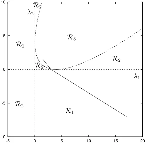
For the triangular configuration λ1 and λ2 are the zeroes of the polynomial
p(λ) = λ2−(α+ 2)λ+βt 4 ,
(see table 1.1). Then, for βt ∈ (0,(α+ 2)2], (λ1, λ2) describes a segment on the plane with endpoints
(α+ 2,0),
µ
α+ 2 2 ,
α+ 2 2
. (4.5)
This segment goes from region R2 toR3 (see figure 4.1) using the notation intro-duced in chapter 2. The change from R2 toR3 takes place when (λ1+λ2−4)2− 4λ1λ2 = 0, that is,
(α−2)2−βt = 0.
For 0 < βt ≤ (α−2)2 the characteristic exponents are ±iω1, ±iω2 and for (α−2)2 < β
t≤(α+ 2)2 they are complex,±a±ib.
Assume 0< βt<(α−2)2. In this case,ω1 6=ω2. To look for resonant points we computeω1,ω2 as
ω21 = 2−α+
p
(2−α)2−β
t
2 , ω
2 2 =
2−α−p
(2−α)2−β
t
2 .
Resonances are obtained when ω1 or ω2 satisfy ωT = nπ for some n ∈ N where T = √2π
2−α or, equivalently when 4ω2 2−α =n
2. Moreover, if 0 < β
t < (α−2)2
then
2< 4ω 2 1
2−α <4, 0< 4ω2
2 2−α <2.
Therefore, we get a unique resonance whenω2T =π forβt=
3
4(2−α) 2.
Let us assume (α −2)2 < βt ≤ (α + 2)2, that is, (λ1, λ2) belongs to the region R3. The characteristic exponents are ±a±ib with b2 =
1
4(2−α+
p
Figure 4.1: Segments corresponding to the collinear and triangular Newtonian case in the plane (λ1, λ2)
A resonance is attained if T b = nπ for some n ∈ N or equivalently 4b 2 2−α = n
2. However for the allowed range ofβtwe get
2< 4b 2 2−α ≤
4 2−α,
that is, in order to have a resonance withT b=nπ we need
2≤n≤ √ 2
2−α. (4.6)
In that case, a simple computation shows that βt = (2−α)2(n2−1)2. We note
that (4.6) has no solution if α < 1. Then, there is no resonance for (α−2)2 < βt < (α+ 2)2 if α < 1. Moreover, we have that
2
√
2−α → +∞ when α → 2
−.
Then, asα≥1 increases we get more resonant points.
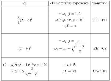
Table 4.1 summarizes the critical values of βt, such that bifurcations are
ex-pected fore >0 small enough.
βt∗ characteristic exponents transition
±iωj, j = 1,2
3
4(2−α)
2 ω
1T 6=nπ, n ∈N, EE↔EH
ω2T =π
±iωj, j = 1,2
(2−α)2 ω
1 =ω2 =
r 2−α
2 EE↔CS
(2−α)2(n2−1)2 for n∈N ±a±ib 2≤n≤ √ 2
[image:7.612.98.455.77.339.2]2−α bT =nπ CS↔HH
Table 4.1: Resonances fore= 0 in the triangular case and expected transitions for small
e
ranges from 0 to 2α+2−1, the point (λ1, λ2) moves on a segment with endpoints (α+ 2,0) ((α+ 1)2α+2+ 1,1−2α+2). (4.7) For βc 6= 0 this segment is contained in the region R1 (see figure 4.1). So, the characteristic exponents are ±λ, ±iω. Only single resonances can be attained when ωT =nπ for somen∈N.
To get the resonant points we write ω2 as
ω2 = 2−α(βc+ 1) +
p
β2
c(α+ 2)2+ 2βc(α2+ 4) + (α−2)2
2 .
It is easy to check thatω2is an increasing function ofβ
c. Then,ω ∈(√2−α, ωM)
being
ωM =
q
1−2α+1α+ 2α2p2α+2(α+ 2)2−8α. (4.8) In terms of n, we have that
2< n < √2ωM
We note that ω2
M → −15 + 8
√
15 > 0 and then √2ωM
2−α → +∞ when α → 2
−.
Then, asα approaches 2, the number of resonances increase.
4.2.2
The Newtonian case
We shall assumeα = 1, that is Newtonian potential. System (4.1) can be written as (2.1) by takingG1 =G2=g−1. The periodic solution of (4.2) isg= 1 +ecosf, where e is the eccentricity of the orbit and f the true anomaly. Then, g−1 = 1−F(f, e) being F(f, e) an even 2π–periodic function on f which satisfies the d’Alembert property. That is, the hypothesis assumed in chapter 2 holds for (4.1).
We begin with the triangular homographic solutions. From table 4.1 we get the following resonant points fore= 0.
βt∗ characteristic exponents 3
4 ±iω1,±iω2, ω1 = √
3 2 ,ω2 =
1 2 1 ±iω1, ±iω2,ω1 =ω2 =
√ 2 2
9 ±a±i
Table 4.2: Resonances fore= 0 in the triangular case for Newtonian potential
We can apply the theory of chapter 2 to the caseβt∗ = 3
4, that is, near the point (a1, a2) =
µ
3 2+
1 4
√
33,3 2−
1 4
√
33
in the plane λ1,λ2. From (2.6), the resonant curve forω1=
1
2 is given by
γt(λ1, λ2) :=
µ
λ1+ 1 4
¶ µ
λ2+ 1 4
[image:8.612.224.413.308.429.2]−1 = 0. (4.9)
Figure 4.2 shows the intersection of the resonant curve (4.9) with the segment with endpoints (4.5).
Figure 4.2: Left: Some resonant curves and the segments corresponding to the triangular and collinear case in the plane (λ1, λ2). Right: Magnification of the triangular case (color
codes are the same as in figure 2.2)
given order inδ1, δ2 and eis
N F = K+ iω1z2z4+ 1
2iz2z4+ iσ1z1z3+iσ2z2z4+ +σ4z22e−it−σ4z42eit,
whereσj ∈R,j= 1,2,4, depend onδ1, δ2 ande. Here,ω1 =
√
3
2 . Then, one of the traces satisfies |tr2|<2 ifδ1, δ2, e are small enough, giving an elliptic component. A region EH is created, and their boundaries are defined by the equation
σ22−4σ42 = 0. (4.10) As we are in a single resonance case and the functionF satisfies d’Alembert prop-erty, we can use the theory in section 2.5.1. In particular, we can compute the dominant terms in the contribution ofδ1 andδ2toσ1. Using lemma 2.5.1, a simple computation shows that
σ1 =
µ
7 2 −
1 2
√
33
δ1+
µ
7 2+
1 2
√
33
δ2+O2.
Now we introduce the parameterδ as in (2.60), that is,
Ã
δ1 δ2
!
whereγ is given in (4.9) and (a1, a2) is the resonant point fore= 0. Then, δ1 =
δ 4(7−
√
33), δ2 = δ 4(7 +
√
33). We can write σ1 in terms ofδ as
σ1 = 41
2 δ+O2,
We have implemented an algebraic manipulator that computes the Normal Form up to a given order inδ1, δ2 and e. In this case, we obtain that
σ4 = −0.035903516541. . . e+O2.
Let us considerδ+(e) andδ−(e) the solutions of the two equations given by (4.10),
that is,σ2−2σ4 = 0 andσ2+2σ4= 0, respectively. We writeδ±(e) =d±e+O(e2).
By proposition 2.5.3, the width of δ+(e)−δ−(e) is of order 1 in e. Moreover, we
can compute explicitly the values ofδ±. We have that
δ±=∓0.0350278210155. . . e+O(e2).
In the plane (λ1, λ2) the boundaries of the region EH are given by λ1 =a1−d1e+O(e2), λ2=a2−d2e+O(e2), λ1 =a1+d1e+O(e2), λ2=a2+d2e+O(e2),
where d1 = 0.0109938087283. . . and d2 = 0.1116035648259. . .. Taking into ac-count that βt = 4λ1λ2 the equations above defines the following curves in the plane (βt, e)
βt−= 3
4 −de+O(e
2), β+
t =
3
4 +de+O(e 2), whered= 0.4903894921666. . ..
We conclude that a resonant tongue T is born at the point (βt, e) =
µ
3 4,0
and the width of T is of order O(e).
[image:10.612.124.478.90.179.2]Remark 4.2.1. The existence of this tongue was proved by G.Roberts in [R.] using a different method.
Figure 4.3 shows the bifurcation diagram on the plane (βt, e) computed
nu-merically. On the range βt ∈(0,9) we distinguish the tongue T born atβt∗ =
3 4. The behaviour fore.1 will be described in section 4.3.
Now we study the collinear case. For e= 0, the characteristic exponents are
0
0.5
1
[image:11.612.114.445.89.330.2]0
3
6
9
Figure 4.3: Bifurcation diagram of the triangular Newtonian homographic solutions in the plane (βt, e). Color codes: Red for EE, Green for EH, Magenta for CS and Blue for
HH
Resonances ω= 3 2,2,
5
2 are found on that range ofβc. The corresponding critical values of βc are given in table 4.3. We expect resonant tongues T3
2, T2 and ,T 5 2 associated to that resonances. Our purpose now is to compute the width of T3 2 and T5
2 using the Normal Form method.
Using the data in tables 4.3 and 1.1, we compute the following resonant points on the planeλ1, λ2,
(a1, a2) =
µ
3 8(
√
41 + 7), 3 16(1−
√
41)
,
(a1, a2) =
µ
1 8(37 +
√
4369),− 1 16(13 +
√
4369)
,
forω= 3
2 and ω= 5
2, respectively. The corresponding resonant curves are γ1(λ1, λ2) =
µ
λ1+ 9 4
¶ µ
λ2+ 9 4
−9 = 0,
γ2(λ1, λ2) =
µ
λ1+25 4
¶ µ
λ2+25 4
β∗
c characteristic width of Tω transition
exponents±iω
3 16(
√
41−1) ω = 3
2 O(e
3) HE←→HH
1 4(1 +
√
97) ω = 2 no bifurcation
1 16(13 +
√
4369) ω = 5
2 O(e
[image:12.612.149.490.77.299.2]5) HE←→HH
Table 4.3: Resonances fore= 0 in the collinear case for Newtonian potential
respectively. Figure 4.2 shows the intersection of the resonant curves with the segment defined by the collinear homographic solutions.
We take λ1 = a1 +δ1 and λ2 = a2 +δ2 with |δ1|,|δ2| small enough. As (a1, a2)∈ R1 the Normal Form up to a given order ofδ1, δ2, eis
N F = K+λz1z3+ iωz2z4+σ1z1z3+ iσ2z2z4+ σ3z22eit−σ3z42eit,
where σ1, σ2, σ3 ∈ R depend on δ1, δ2 and e, and (λ, ω) =
µ
1 4
q
3√41 + 17,3 2
or
µ
1 4
q
97 +√4369,5 2
. We have that |tr1| > 2. A region HH is created. Its boundaries are defined by the equation
σ22−4σ23 = 0.
We takeβc =βc∗+δ. Then, δ1 = 2δ and δ2 =−δ. We are in a single resonance case. Moreover, function F satisfies d’Alembert property. Then, using lemma 2.5.1 we obtain that
σ2 =
53√41−123
610 δ+O2 if ω= 3 2, σ2 =
197√4369−4369
Using the algebraic manipulator we obtain that
σ3 = −5.9623466927. . .·10−3e3+O4 if ω = 3 2, σ3 = −3.3038513137. . .·10−5e5+O6 if ω = 5
2.
Let us consider δ+(e), δ−(e) the solutions of σ2 −2σ3 = 0 and σ2 + 2σ3 = 0, respectively. If we write δ±(e) =d±1e+d±2e2 +d±3e3+d±4e4+d±5e5+O(e6) and taking into account the expression up to order 3 and 5 in the case ω = 3
2 and ω = 5
2, given by the algebraic manipulator, we obtain that the boundaries of the resonant tongues in the plane (βc, e) are given by
βc−βc∗ = −0.4208699384. . . e2±0.03361931602. . . e3+O(e5) if ω=
3 2, βc−βc∗ = −1.9578203867. . . e2−0.5109418802. . . e4
±0.00032876661. . . e5+O(e6) if ω= 5 2, where we recall thatβc−βc∗ =δ.
Therefore, two resonant tonguesT3 2 andT
5
2 are born ate= 0 being their width of ordere3,e5, respectively (see table 4.3).
In the case ω = 2 the computations up to a given order using the algebraic manipulator shows that the two boundaries coincide up to that order. We prove now that, in fact, if ω = 2 there is no bifurcation. To this end, we consider the system (4.1) in the Newtonian case for arbitrary (λ1, λ2)∈ R1∪ R2.
Lemma 4.2.2. Let us consider the system (4.1) in the Newtonian case and assume that for e= 0, (λ1, λ2) = (a1, a2) ∈ R1∪ R2, we get a single resonance frequency ω = n with n ∈ N. Then, the two boundaries of the resonant region coincide. There is no bifurcation in this case.
Proof
Forω =n,n∈N, one stability parameter, tr2, is equal to 2 fore= 0. Then the boundaries of the resonant region are defined by tr2 = 2. Furthermore, if (λ1, λ2, e) belongs to the boundary, the linear system (4.1) has a 2π–periodic solution. To finish the proof we need the following lemma.
Lemma 4.2.3. Assume that (4.1) has a 2π–periodic solution, ϕ, for a fixed value of e ∈ (0,1) and λj 6= 0, j = 1,2. Then, there exists a second periodic solution
Now we prove Lemma 4.2.2.
Let us define Φ(2π) the monodromy matrix of (4.1). After lemma 4.2.3, if (λ1, λ2, e) belongs to the boundary of the resonant region then Φ(2π) can be written (in a suitable basis) as
Φ(2π) =
Ã
Q 0 0 I2
!
,
for some 2×2 matrix Q. Using the Normal Form we can compute Φ(2π) up to a given order in δ1, δ2, e. As we are in a single resonance case we know that the reduced system becomes uncoupled. Assume that (a1, a2) ∈ R1. Then the subsystem that defines tr2 is (2.39), that is,
˙
u = iσ2u−2σ3v, ˙
v = −2σ3u−iσ2v.
(In the case (a1, a2) ∈ R2 a similar subsystem is obtained). We define for this system the symplectic change of coordinates
à η1 η2 ! = √ 2 2 à 1 i i 1 ! à u v ! .
Then the new system is
à ˙ η1 ˙ η2 !
= S1
Ã
η1 η2
!
,
whereS1 =
Ã
0 σ2−2σ3
−(σ2+ 2σ3) 0
!
. The corresponding monodromy matrix is exp(2πS1).
Let us assume that (λ1, λ2, e) belongs to the boundary such thatσ2−2σ3 = 0. Then,S1 =
Ã
0 0
−(σ2+ 2σ3) 0
!
and exp(2πS1) =
Ã
1 0
−2π(σ2+ 2σ3) 1
!
. If for these values of the parameters, σ2+ 2σ3 6= 0, then system (4.1) would have a unique 2π–periodic solution. This gives a contradiction with lemma (4.2.3). In this way we have proved that the two boundaries coincide up to arbitrary order in e, once δ1 = δ1(e) and δ2 = δ2(e). Using the analycity they coincide for any value of the eccentricity. ✷
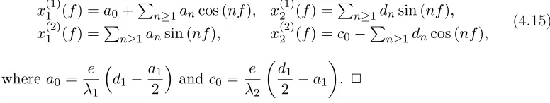
Proof of Lemma 4.2.3
System (4.1) can be written as the following system of second order equations (1 +ecosf)¨x1 = λ1x1−2 ˙x2(1 +ecosf),
A 2π–periodic solution of the system above can be written as x1(f) = a0+
X
n≥1
ancos(nf) +
X
n≥1
bnsin(nf),
x2(f) = c0+
X
n≥1
cncos(nf) +
X
n≥1
dnsin(nf). (4.12)
Then, the coefficients must satisfy the following uncoupled sets of recurrences λ1a0 =e
³
d1− a1 2
´
,
eA2u2 =B1u1, (4.13)
eAn+1un+1=Bnun−eAn−1un−1, n≥2, u= (an, dn)T,
λ2c0=−e
³
b1+c1 2
´
,
eA2Sv2=B1Sv1, (4.14) eAn+1Svn+1 =BnSvn−eAn−1Svn−1, n≥2, v= (bn, cn)T,
whereAn=−
n 2
Ã
n −2
−2 n
!
,Bn=
Ã
λ1+n2 −2n
−2n λ2+n2
!
andS = diag(1,−1). We note that if un,n≥1 is a non trivial solution of the last two equations in
(4.13) then vn=Sun= (an,−dn)T, n≥1, is a non trivial solution of the second
and third equations in (4.14). Moreover, An is a non singular matrix for n > 2.
However, det(A2) = 0. But if det(B1) = (λ1 + 1)(λ2 + 1)−4 6= 0, given u2 we can compute u1 from the second equality in (4.13), and from the last equation we obtain un forn≥3.
We assume that (4.12) is a non trivial 2π–periodic solution of (4.11). Then, both (4.13) and (4.14) have a solution. We assume that (4.13) admits a non trivial solution. Then,P
n≥1ancos (nf) and
P
n≥1dnsin(nf) are convergent. Therefore
vn=Sun, that is, bn=anand cn=−dn, forn≥1, is a solution of (4.14). Then,
we can built two independent periodic solutions of (4.11) as
x(1)1 (f) =a0+Pn≥1ancos (nf), x(1)2 (f) =Pn≥1dnsin (nf),
x(2)1 (f) =P
n≥1ansin (nf), x(2)2 (f) =c0−Pn≥1dncos (nf),
(4.15)
wherea0 = e λ1
³
d1− a1
2
´
and c0= e λ2
µ
d1 2 −a1
[image:15.612.81.469.540.613.2]. ✷
Figure 4.4 shows the bifurcation diagram on the plane (βc, e) computed
nu-merically forβc ∈(0,7), e∈[0,1). The first tongue borns atβc∗=
3 16(
√
41−1) = 1.013. . .. We recall that the width of T3
2 is of order e
boundaries we have to look at big values of the eccentricity. In figure 4.4 the line inside the resonant tongue corresponds to a minimum of the stability parameter. The second ’tongue’, T2, is only a curve defined by points (βc, e) for which the
second stability parameter is equal to 2, as predicted by lemma 4.2.2. For the third tongueT5
2 the width is of ordere
5. We can distinguish the two boundaries in figure 4.5 which is a magnification of 4.4 for big values of e. Other curves in figures 4.4 and 4.5 are resonant tonguesTω for ω= m
2, m∈N,m >5. They are born at values β∗c > 7. The behaviour of Tω as e goes to 1 will be described in
section 4.3.
0 0.2 0.4 0.6 0.8 1
[image:16.612.161.474.230.453.2]0 1 2 3 4 5 6 7
Figure 4.4: Bifurcation diagram of the collinear Newtonian homographic solutions in the plane (βc, e)
4.2.3
The general case
For the general case we do not know explicitly the expression of gα−2. In this section we shall see that system (4.1) satisfies the properties of system (2.1). Then, the theory in this chapter can be applied for the homographic solutions in the general case. Moreover, we will see that gα−2 satisfies d’Alembert property, and then we can compute as in 2.5 the boundaries of the resonant regions.
0.99 0.992 0.994 0.996 0.998 1
[image:17.612.120.432.81.306.2]0 1 2 3 4 5 6 7
Figure 4.5: Magnification of the bifurcation diagram of the collinear Newtonian homo-graphic solutions in the plane (βc, e)
of v is ¨
v= 2(α−2)(α−3)E(v+ 1)2−4−αα + (α−2)2(v+ 1)
µ
3
α(v+ 1)−1
, (4.16)
whereE denotes the energy of (4.2), that is,E= z˙
2 +U(z).
Let e > 0 be small enough. We look for a solution of (4.16) which satisfies initial conditionsv(0) =eand ˙v(0) = 0. We shall write
v(f) = v1(f)e+v2(f)e2+v3(f)e3+. . . , (4.17) where v1(0) = 1, vj(0) = 0 for j ≥ 2 and ˙vj(0) = 0 for j ≥ 1. We remark that
writing the energy of (4.2) in terms of v we have that E = 1
2(e+ 1) 2
α−2 − 1
α(e+ 1) α
α−2 =E1+ ∆, E1=−2−α
2α , (4.18) and ∆ =α2e2+α3e3+α4e2+O(e5) with
α2= 1
2(2−α), α3=−
4−α
3(2−α)2, α4=
(4−α)(3−α) 4(2−α)2 , . . .
To get v(f) we use a Lindstedt–Poincar´e method. So, we introduce a new inde-pendent variableτ =νf with
The coefficientsνj,j≥0 will be determined in order to eliminate resonant terms.
Using (4.18) the equation (4.16) can be written as
ν2d 2v
dτ2 = f(v) +g(v)∆, (4.19) where
f(v) = E1g(v) + (α−2)2(v+ 1)
µ
3
α(v+ 1)−1
,
g(v) = 2(2−α)(3−α)(v+ 1)4−2−αα.
By substituting (4.17) in (4.19) we get
ν02d 2v
1
dτ2 =−(2−α)v1, v1(0) = 1, dv1
dτ (0) = 0. We chooseν2
0 = (2−α) and then trivially v1(τ) = cosτ. In a similar way we get v2(τ) = 1
2(2−α) +
α−4
3(2−α)cosτ−
2α−5
6(2−α)cos (2τ), v3(τ) = α−4
3(α−2)2 +
µ
(α−4)(7−α) 9(2−α)2 −
9α2−47α+ 62 96(2−α)2
cosτ
−(2α9(2−5)(α−4)
−α)2 cos (2τ) +
9α2−47α+ 62
96(2−α)2 cos (3τ), ν1= 0 and
ν2 = −
√
2−α 2(2−α)2
µ
1
6(2α−5)(11−2α)− 3
4(α−3)(4−α)
.
In this way we can obtain g2−α = 1 +v(τ) up to a given order. Then, g2−α = 1 +v(νf) is a periodic function off with periodT = 2π
ν .
Now we shall see thatg2−αis an even function offand satisfies the d’Alembert property.
Lemma 4.2.4. Let v(τ) = P
m≥1vm(τ)em be the solution of (4.19) such that
v1(0) = 1,vj(0) = 0forj≥2andv˙j(0) = 0forj≥1. Then,vm(τ),m∈N, is an
even function on τ which satisfies the d’Alembert condition, that is, form∈N, vm(τ) =
m
X
l=0
Proof
We know that g(f) is an even periodic function of f. So, v(τ) is also an even function. Moreover v1(τ) = cosτ. Assume that vm(τ) for m= 1,2, . . . , k−1 are
known and satisfy the (4.20). If we define w=eiτ then vm(τ) contains terms wl
withl≤m.
The equation for vk(τ) is obtained by equating in (4.19) terms of orderkine.
It is clear that v1(τ), . . . , vk−1(τ) give terms withwl, withl≤k−1, in ¨v.
Concerning the right part of (4.19) to get the terms of orderk inefrom f(v) it is sufficient to consider
f(v) = f′(0)vk(τ) + k
X
j=2
f(j)(0) j! (v
(k))j,
wherev(k)(τ) =v1(τ)e+. . .+vk(τ)ek.
The terms of order kinewhich come from (v(k))j can be written as (v(k))j = X
l1+. . .+lk=j,
l1+ 2l2+. . .+klk=k
vl1
1vl12· · ·vlkkek. (4.21)
In (4.21) we considerj≥2. This implieslk= 0 in the summatory (4.21). Using the
hypothesis onv1(τ), . . . , vk−1(τ) we get that the highest term inw which appears invl1
1vl22· · ·vlkk iswl1+2l2+...+(k−1)lk−1 =wk. In a similar way it can be proved that
g(v)∆ contributes to the equation of vk with terms wl, l ≤k−2. Therefore we
can write the equation forvk(τ) as a linear non homogeneous differential equation
ν02¨vk = f′(0)vk+F(τ),
where F(τ) depends on v1(τ), . . . , vk−1(τ). The terms of F(τ) contain wl with l≤k. This proves the lemma. ✷
4.3
Stability parameters near the singular case
Our purpose in this section is to apply the theorem 3.3.1 to the system (4.1). First we note that using (4.3) we obtain ˆλ=−(2−α)
2
8α . Moreover we recall that the parameterδ in theorem 3.3.1 is related to the generalized eccentricity through (4.4). So, we are interested now in small δ > 0. We shall assume that the non degeneracy conditions of theorem 3.3.1 are satisfied.
is,βc 6=
(2−α)2
2α . The parameters β1,β2 in the theorem are easily computed (see table 4.4).
α∈(0,2) α= 1
β1 1 2−α
p
8α(α+ 1)βc+ (3α+ 2)2 √25 + 16βc
β2
s
1− 8αβc (2−α)2
√
[image:20.612.180.456.126.274.2]1−8βc
Table 4.4: The parametersβ1,β2 in theorem 3.3.1 for the collinear case
We remark that in the caseα= 1 the values of βj,j= 1,2, are related to the
eigenvalues of the equilibrium points on the triple collision manifold (see [Mo.2]). We note that β1 >0. Then tr1 > 2 if δ >0 is small enough. Furthermore if βc <
(2−α)2
8α , β2 ∈ R and the second stability parameter is greater than 2. In this case, the system is hyperbolic–hyperbolic for δ > 0 small enough. On the other hand, ifβc>
(2−α)2
8α thenβ2 is pure imaginary. From (3.14) we know that tr2 oscillates asδ tends to 0.
In the Newtonian case the behaviour of tr2 changes at βc =
(2−α)2 8α =
1 8 = 0.125. We have computed numerically tr2 as a function of the eccentricity for several values ofβc. Their plots are represented in figure 4.6 by taking−log10(1−e) on thexaxis. The computations shows that ifβc<
1
8, tr2 goes to−∞. However, if βc >
1
8, tr2oscillates between 2 and a negative valuek <−2. Moreover numerically we see thatk decreases as βc →
µ
1 8
¶+
. As tr2 goes beyond−2, several intervals on eof hyperbolic–hyperbolic (HH) type are created. Therefore, for a fixed βc =
b with b > 1
8 we must have on the bifurcation diagram a sequence of infinite intervals of type HH which accumulate at e = 1. These HH intervals are in fact the intersections of the infinitely many resonant tongues Tω with the line βc =b
(see figure 4.5). This implies that Tω with ω = m
2, m ≥ 4 tends to βc = 1 8 as e tends to 1.
Figure 4.6: Stability parameter tr2in the collinear Newtonian case for several values of
βc. −log10(1−e) is taken on thexaxis
function of βc when e is near 1. The plot corresponds to e = 1−10−4. We
distinguish clearly the first interval with tr2<−2 when βc is small. This interval
corresponds to the first tongue T3
2. In the following oscillations the parameter goes under−2 by a small quantity defining the successive tongues. The numerical computations show that the first minimum goes to infinity asegoes to 1.
It is also interesting to point out that figures 4.6 and 4.7 show that tr2does not cross the horizontal line tr2 = 2, which corresponds to resonances ω =n, n∈N. This means that there is no bifurcation when ω = n (the two boundaries of Tn
coincide) as it was predicted by lemma 4.2.2.
Now we consider the triangular case. From table 1.1 we get λ1 > λ2 >0 and theorem 3.3.1 holds. The parametersβ1,β2 in the theorem are given in the table 4.5.
Now, β1 ∈ R, β2 ∈ R. Then, if δ > 0 is sufficiently small the system is HH provided that the coefficient d1 in theorem 3.3.1 is different from 0. From lemma 3.3.5 we know that d1=dndg where dn 6= 0 anddg depends on the potential and
-8 -7 -6 -5 -4 -3 -2 -1 0 1 2
[image:22.612.138.497.84.340.2]0 1 2 3 4 5 6
Figure 4.7: Behaviour of tr2 fore= 0.9999 in the plane (βc,tr2)
Figure 4.3 shows the bifurcation diagram for the triangular Newtonian homo-graphic solutions in the parameter spaceβt, e. We see that for e.1, the system
is HH for any βt except in a neighbourdhood of some critical value ˜βt near 6.
Numerical computations ofdg seems to indicate that it is equal to zero. However
we do not have a proof of this fact.
0 0.5 1
0 1 2 3 4 0
0.5 1
0 1 2 3 4
0 0.5 1
0 2 4 6 0
0.5 1
0 2 4 6 8
0 0.5 1
0 3 6 9 0
0.5 1
[image:23.612.104.450.158.521.2]0 3 6 9 12
Figure 4.8: Bifurcation diagram for the triangular homographic solutions. The values of α are: top file α = 0.01, α= 0.1; center fileα = 0.5, α= 0.9; bottom file α = 1.1,
α ∈(0,2) α= 1
β1
s
1 + 4α(2 +α)
(2−α)2 (1 + ˜γ) √
13 + 12˜γ
β2
s
1 + 4α(2 +α)
(2−α)2 (1−˜γ) √
[image:24.612.207.430.267.428.2]13−12˜γ
Table 4.5: The parameters β1, β2 in theorem 3.3.1 for the triangular case where ˜γ = √
Some heteroclinic connections
in the Spatial RTBP
In this chapter we study analytically the existence of homoclinic orbits to the centre manifold of the Spatial Restricted Three Body Problem (SRTBP).
The SRTBP has five relative equilibrium points, two triangular and three collinear. The collinear relative equilibrium points are of centre–centre–saddle type and then have 1–dimensional stable and unstable invariant manifolds and a 4–dimensional centre manifold.
In a neighbourhood of the collinear equilibrium points there are two families of Lyapunov periodic orbits, the planar and the vertical families. A Lyapunov periodic orbit has 2–dimensional stable and unstable invariant manifolds. There also exist 2–dimensional invariant tori with 3–dimensional stable and unstable invariant manifolds.
We shall study the existence of homoclinic orbits to the centre manifold of one of the relative equilibrium points. To this end, we consider the SRTBP as a perturbation of the three dimensional Hill’s problem and also as a perturbation of the spatial synodic two body problem.
For the existence of homoclinic orbits on small perturbations of integrable system under generic assumptions see [L.], [K.L.1], [K.L.2].
5.1
The Spatial Restricted Three Body
Prob-lem
Let us consider two bodies, called primaries, describing circular orbits in the plane (x, y) around their center of masses that we assume located at the origin. If we
consider a system of coordinates that rotates with the primaries and suitable units, the bodies can assumed to have massesm1= 1−µ and m2 =µ, with µ∈
¡
0,12¤
, and to be fixed located at coordinates (µ,0,0) and (µ−1,0,0), respectively. It can also be assumed that they complete one inertial revolution in 2π time units.
It is well known that the equations of motion of a massless particle under the gravitational action of the primaries are
¨
x−2 ˙y = Ωx,
¨
y+ 2 ˙x = Ωy, (5.1)
¨
z = Ωz,
where
Ω(x, y, z) = 1 2(x
2+y2) +1−µ r1
+ µ r2
+ 1
2µ(1−µ), (5.2)
r12 = (x−µ)2+y2+z2, r22 = (x−µ+ 1)2+y2+z2. (5.3) Equations (5.1) are called the equations of the spatial restricted three body prob-lem.
Equations (5.1) have a first integral , called theJacobi integral, given by F(x, y, z,x,˙ y,˙ z) =˙ −( ˙x2+ ˙y2+ ˙z2) + 2Ω(x, y, z). (5.4) They also have the following symmetry
S(x, y, z,x,˙ y,˙ z, t) = (x,˙ −y, z,−x,˙ y,˙ −z,˙ −t), (5.5) It is well known that system (5.1) has five equilibrium points, three collinear pointsL1, L2, L3, located on thex axis, and two triangular points,L4, L5 forming an equilateral triangle with the masses and located at the x, y plane. Figure 5.1 shows the equilibrium points of the SRTBP in the plane (x, y). If we denote by Ci the value of (5.4) on the Li points, i= 1, . . . ,5, we have that 3 =C4 =C5 ≤ C3 < C1 < C2<4.25 for all µ∈¡0,12¢.
Let us denote by M(µ, C) the hypersurface given by
M(µ, C) ={(x, y, z,x,˙ y,˙ z)˙ ∈R6| F(x, y, z,x,˙ y,˙ z) =˙ C}. (5.6) Due to the existence of the Jacobi integral, we can restrict to study the behaviour of the orbits inM(µ, C). The projection ofM(µ, C) in the position space (x, y, z) is called Hill’s region. We shall denote it by
Figure 5.1: Equilibrium points of the SRTBP in the plane (x, y)
The boundary ofR(µ, C) is the surface of zero velocity. ForC > C2 Hill’s region consists in two ovoids enclosing the two primaris and a cilindrical surface outside the ovoids. We denote byRb(µ, C) the bounded components of the Hill’s region.
In this case, Rb(µ, C) is formed by the two ovoids. As the value of C decreases
the ovoids inRb(µ, C) meet at L2 (see figure 5.2). The three dimensional picture
Figure 5.2: Intersections of Rb(µ, C) forC=C2 in the planes (x, y) and (x, z),
respec-tively, forµ= 0.2
[image:27.612.81.473.437.572.2]a sphere. In this case Rb(µ, C) has a unique connected component and so, it is
[image:28.612.136.504.137.276.2]possible that the massless particle travels from a neighbourhood of a primary to a neighbourhood of the other primary (see figure 5.3). We denote by Mb(µ, C) the
Figure 5.3: Intersections ofRb(µ, C) forC.C2 in the planes (x, y) and (x, z),
respec-tively, forµ= 0.2
component ofM(µ, C) that projects inRb(µ, C). We shall study the behaviour of
the orbits inMb(µ, C) for C.C2.
5.1.1
Qualitative description of a neighbourhood of
L
2As we are interested in the orbits near L2, we shall give a qualitative description of a neighbourhood of this point. For details see [Sz.]. In fact, the same arguments hold for the other collinear equilibrium points.
By introducing momenta as px = ˙x−y, py = ˙y+x and pz = ˙z, the SRTBP
can be written in Hamiltonian form, and the Hamiltonian function is H(x, y, z, px, py, pz) =
1 2(p
2
x+p2y+pz2)−xpy+ypx−
1−µ r1 −
µ r2
, (5.8) wherer1 and r2 are defined in (5.3). The relation between the energy h and the Jacobi constant of an orbit is given by
C=−2h−µ(1−µ).
L2 is located between the two primaries (see figure 5.1). We introduce ρ by r2 =ρ. Then, r1 = 1−ρ and x=µ−1 +ρ for this equilibrium point. Figure 5.4 shows the situation.
ρ is the solution of Euler’s quintic equation
Figure 5.4: Coordinates ofL2
The linearized equations around the collinear equilibrium point are given by the second order terms of the Hamiltonian. These terms can be written as
H2 = 1 2(p
2
x+p2y)−xpy+ypx−c2x2+ c2
2y 2+1
2p 2
z+
c2 2z
2, (5.10)
where c2 =
1−µ (1−ρ)2 +
µ
ρ3. Figure 5.5 shows the values of c2 depending on the parameterµ.
Figure 5.5: Values of c2 depending onµ
From the expression ofH2 it is clear that, linearly, the directionzis uncoupled from the planar directions. The linearized system forz,z˙ is an harmonic oscillator with frequency ωv =√c2. It is well–known that ωv ∈ (2,3) (see figure 5.6). For
[image:29.612.89.449.219.558.2]is
p(λ) =λ4+ (2−c
2)λ2+ (1 +c2−2c22). Then, if we denote byη =λ2, the zeroes ofp(λ) are given by
η1,2 =
c2−2±
p
9c2 2−8c2
2 ,
[image:30.612.155.480.258.504.2]where, according to the values of c2, η1 > 0 and η2 < 0. Then, L2 is a centre– centre–saddle point. The frequencyωp =√−η2 is known as planar frequency. It is easy to see thatωp ∈(2,3). Figure 5.6 shows the graphic ofωp in terms of µ.
Figure 5.6: Frequencies ωp andωv in terms ofµ∈
µ
0,1
2
AsL2 is of centre–centre–saddle type, it has 1–dimensional stable and unstable manifolds and a 4–dimensional centre manifold. Fixed an energy level C of the Jacobi constant, Wc
L2 ∩M(µ, C) is homeomorphic to S
3, where Wc
L2 denotes the centre manifold of L2 (see appendix D).
These families are hyperbolic, and they have 2–dimensional stable and unstable invariant manifolds. We remark that the planar family of periodic orbits also exists in the Planar Restricted Three–Body Problem. Therefore, the stable and unstable invariant manifolds of the planar periodic orbits lie onz= 0,z˙= 0.
For the linearized SRTBP and fixed C, the centre manifold, WLc2 ∩M(µ, C) is foliated by a one parameter family of 2–dimensional invariant tori. Generically, using KAM theory most of these tori subsist for the general SRTBP. Moreover, the tori have 3–dimensional stable and unstable invariant manifolds.
5.2
Homoclinic connections in the planar case
The Planar Restricted Three Body Problem is obtained from the equations of the SRTBP by taking (z,z) = (0,˙ 0). In this case, on a neighbourhood of L2 and for values of C ≤ C2 there also exist the planar family of Lyapunov periodic orbits. In this case, they have two–dimensional stable and unstable invariant manifolds, that we shall denote byWp.o.s andWp.o.u , respectively. The existence of transversal homoclinic orbits in the planar problem for µ&0 and C . C2 has been studied in [L.M.S.]. In this section we shall summarize some of the results obtained in [L.M.S.].
In this case, we consider the hypersurface defined by ˜
M(µ, C) =M(µ, C)|(x,x,y,˙ y,˙0,0).
The Hill’s region ˜R(µ, C) is the projection of ˜M(µ, C) in the position space. Let us consider ˜Rb(µ, C) the bounded components ofR(µ, C). We have that forC =C2,
˜
R(µ, C) is formed by two connected components that have a contact point in L2 (see the left figure in 5.2). We shall denote by S the connected component that contains the larger primary. For C ≤C2 we can take two segments in ˜Rb(µ, C)
joining points in the zero velocity curve (see figure 5.7) that divides the region in three components. One of the components contains the projection of the periodic orbit near L2, and the other components contain one of the primaries each one. Naming ˜Mb(µ, C) the component of ˜M(µ, C) that projects on ˜Rb(µ, C), we shall
denote again the component that contains the large primary asS. The main result in [L.M.S.] is the following.
Theorem 5.2.1. 1. For values of µ & 0 of the form µk =
1 N3
∞k3
(1 +o(1)), whereN∞ is a suitable constant ando(1)denotes terms that go to zero when
µ does, there exists an homoclinic orbit toL2.
2. If µ and ∆C = C2−C > 0 are small enough, the branch Wp.o.u,S of Wp.o.u
Figure 5.7: Hill’s region in the Planar Restricted Three Body Problem for C.C2and
regionS
diffeomorphic to a circle. In particular, for the points in theµ, C plane such that there existsµk satisfying∆C > Lµ
4 3
k(µ−µk)2, beingL a constant, there
exist transversal symmetric homoclinic orbits to the periodic orbit.
5.3
Statement of the results in the Spatial
case
Fixed a valueC of the Jacobi constant, from (5.4) we have that
C = F(x, y, z,x,˙ y,˙ z).˙ (5.11) This is equivalent to fix a level hypersurface of the form (5.6). We shall denote as Cp the constant that one obtains from (5.11) by taking z= 0,z˙= 0, that is,
Cp = F(x, y,0,x,˙ y,˙ 0). (5.12)
Then, Cp is the Jacobi constant of the Planar problem. We shall refer to it as
planar component of the Jacobi constant. We define Cv by
Cv = C−Cp, (5.13)
and when talking about this constant we shall say vertical component of the Jacobi constant. Then, we have written the Jacobi constant as the sum of a planar component and a vertical one.
Let be ∆C =C2−Cp and define
∆Cp =C2−Cp, ∆Cv =−Cv,
We introduce constantsα,β by
µ = µk+αµ
4 3
k,
∆C = βµ43
where µk is defined in Theorem 5.2.1 and α, β =O(1) depend on µk. Once µ is
fixed we can takeµk as the value of the sequence given by Theorem 5.2.1 which is
at minimum distance to µ. We defineψ∈h0,π 2
i
by
∆Cp =βcos2(ψ)·µ
4 3
k, ∆Cv =βsin2(ψ)·µ
4 3
k. (5.15)
We note that once ∆C >0 is fixed, ifψ= 0 then ∆C = ∆Cp which corresponds
to the planar problem. Forψ= π
2 then ∆C = ∆Cv.
Given α andβ, a torus in the centre manifold ofL2 is characterized by ψ.
The following theorem gives the existence of heteroclinic orbits between two tori provided some inequalities are satisfied. Some non degeneracy conditions will be required in the sense that A 6= 1 and C1 6= 0 for some coefficients to be introduced in section 5.4. The geometrical meaning is that some ellipse in the (z,z) plane taken in the initial conditions of˙ WTu,µ does not degenerate into a cercle and its axes do not coincide with the z, ˙z axes. Here, WTu,µ denotes the unstable manifold of an invariant torus T in the centre manifold of L2 once the Jacobi constantC.C2 is fixed.
Theorem 5.3.1. Let us considerα, β fixed andµk sufficiently small. Assume non
degeneracy conditions. Let be ψ, ψ′ ∈³0,π 2
´
\ E, being E a set of small measure, such that
cosψ,cosψ′> √K
β|αˆ−k|, (5.16)
for some integer k, where K > 0 is a constant and |αˆ|=
¯ ¯ ¯ ¯
α 3N∞
¯ ¯ ¯ ¯ ≤
1
2. Let be m the number of integersk such that (5.16) is satisfied and assume
sinψ sinψ′ ∈(κ
−1, κ), (5.17)
where κ > 1 is a constant. Then there exist 16m transversal heteroclinic orbits between the tori characterized byψ and ψ′.
In particular, there exist at least 16m homoclinic orbits to the centre manifold.
Remark 5.3.2. The constantsKandκare effectively computed in section 5.4. They depend on the parameters of some ellipses in the planesx,x˙ and z,z, respectively.˙
Assume K|√αˆ|
β <1. Let be ψmax= arccos
µ
K √
β|αˆ|
. Ifψ, ψ′ ∈(0, ψmax) then
(5.16) holds at least fork= 0. This situation is represented in figure 5.8.
Figure 5.8: Admissible values ofψ
Furthermore, ifψ and ψ′ satisfy (5.17), then there exists an heteroclinic orbit from the torus characterized by ψto the one characterized by ψ′.
Notice that if ˆα = 0 then µ= µk. In this case (5.16) is satisfied trivially for
k = 0. Moreover as β increases, (5.16) holds for other values of k. This is in agreement with the previous results in the Planar RTBP ([L.M.S.]).
Notation 5.3.3. Forψ, ψ′ ∈³0,π 2
´
we shall denote by
ψ−→ψ′
the existence of an heteroclinic orbit between the tori characterized byψ andψ′.
Corollary 5.3.4. We fix α, β such that K|√αˆ|
β <1. If ψ1, . . . , ψn, . . .∈
¡
0,π2¢
is a
sequence of values such that
ψn∈(0, ψmax),
and
sinψn
sinψn−1 ∈
(κ−1, κ), then
ψ1−→ψ2 −→ψ3 −→. . . .
5.4
Proof of Theorem 5.3.1
In order to obtain homoclinic connections to the centre manifold of L2 we follow the same ideas given in [L.M.S.].
Let us denote byWTu,µthe unstable manifold of an invariant torusT on a level manifoldM(µ, C) with C.C2(µ) of the SRTBP. In order to prove theorem 5.3.1 we shall obtain an analytic expression for this invariant manifold when µ&0 to obtain later heteroclinic and homoclinic orbits to the torus. Our purpose is to obtain the first intersection of WTu,µ with Σ ={y = 0, x >0}. We shall assume that Σ is a Poincar´e section for any orbit of WTu,µ. Due to the transversality of WLu,µ
2 with Σ, this assumption holds if ∆C is sufficiently small. In order to obtain this intersection, we shall approximate the SRTBP by the spatial Hill’s problem in a neighbourhood of the equilibrium point. Then, as outside of a neighbourhood of L2 the SRTBP can be seen as a perturbation of the Spatial Two Body Problem, we shall use it in order to obtain the expression ofWTu,µ∩Σ. Once this intersection is obtained, we shall use the symmetries of the equations in order to obtain the stable manifold. Then, studying the intersections of the unstable manifold of one torus and the stable manifold of another torus, we shall obtain heteroclinic orbits. By taking the unstable and stable manifolds of the same torus we will obtain homoclinic orbits to that torus.
5.4.1
Geometry in a neighbourhood of the equilibrium
point
In order to study the geometry of the unstable manifold in a small neighbourhood of the equilibrium point, we shall consider the intersection of this manifold with the sectiony=−kµ13, wherek is large enough ambµsufficiently small, in such a way thatkµ13 is small enough. To this end we shall approximate the equations of the SRTBP by the Spatial Hill’s problem in a neighbourhood of the equilibrium point. If (X, Y, Z) denotes the coordinates of the Spatial Hill’s problem, then we need to study the geometry of the invariant manifold in the sectionY =−k, with k large enough. The analysis of the Poincar´e map between two sections Y =−k˜ and Y = −˜˜k, 0 < ˜k < k, with ˜˜˜ k large enough, will give us the geometry of the manifold intersected with different hyperplanes.
Near the small mass µ, in suitable coordinates the SRTBP can be seen as a µ13 order perturbation of the Spatial Hill’s problem. The three–dimensional Hill’s problem studies the behaviour of the small mass for the SRTBP in the limit case when µ → 0. To obtain the limit equations we translate the small mass to the origin and we perform a scaling of the variables by the change of coordinates (x, y, z)−→(X, Y, Z) defined by
X=µ−13(x+ 1−µ), Y =µ− 1
3y, Z =µ− 1
3z. (5.18) Then, equations (5.1) can be written as the second order system
¨
X−2 ˙Y = 3X−X(X2+Y2+Z2)−32 +µ 1 3
µ
3X2− 3 2Y
2− 3 2Z
2
+O(µ23), ¨
Y + 2 ˙X = −Y(X2+Y2+Z2)−32 −3µ 1
3XY +O(µ 2 3), ¨
Z = −Z−Z(X2+Y2+Z2)−32 −3µ 1
3XZ+O(µ 2 3).
If we take µ= 0 we obtain the equations for the 3–dimensional Hill’s problem ¨
X−2 ˙Y = 3X−X(X2+Y2+Z2)−32, ¨
Y + 2 ˙X = −Y(X2+Y2+Z2)−32, (5.19) ¨
Z = −Z−Z(X2+Y2+Z2)−32. We note that equations (5.19) can be written as
¨
X−2 ˙Y = ΩHX, ¨
Y + 2 ˙X = ΩHY, (5.20) ¨
with
ΩH(X, Y, Z) = 1 2
h
3X2−Z2+ 2(X2+Y2+Z2)−12
i
.
Equations (5.19) have a first integral
FH(X, Y, Z,X,˙ Y ,˙ Z) = 2Ω˙ H(X, Y, Z)−( ˙X2+ ˙Y2+ ˙Z2) =CH. (5.21) As we have done with the Jacobi constant for the SRTBP, we can consider the value of the integral,CH, as a sum of a planar and a vertical component. We shall write
CH = CpH +CvH, (5.22) beingCpH =FH(X, Y,0,X,˙ Y ,˙ 0) the planar component andCvH the vertical one.
The only two equilibrium points of the 3–dimensional Hill’s problem are collinear. If we denote byL1andL2these equilibrium points, we have thatL1= (−3−
1 3,0,0) and L2 = (3−
1
3,0,0). The use of this notation is due to the fact that Lj for the Spatial Hill’s problem corresponds to Lj for the SRTBP. Using (5.21) we obtain
CH Lj = 3
4
3 for the collinear equilibrium points. We shall consider L2. The eigen-values for the linerized system at L2 are ±λ, ±iω, ±2i where λ =
p
1 + 2√7, ω=p2√7−1. Then it is a centre–centre–saddle point.
We denote byWLu,H2 the one–dimensional unstable manifold ofL2. It is known (see [L.M.S.], [McG.1]) that one of the branches ofWLu,H2 crosses the lineY =−k, for any valuek >0 going down forwards, near the surface of velocity zero. More-over, as in the SRTBP, there exist two families of periodic orbits in a neighbour-hood ofLH
2 , the planar and the vertical families. Furthermore using the KAM the-orem, generically there exist invariant tori in the centre manifold of the collinear points.
For a fixed CH ≤ CLH2 = 343 we take ∆CH = CH
L2 −C
H. Let us consider a
solution of the linearized Spatial Hill’s Problem on the centre manifold of L2. It can be written as
X(t) = 2ωacos (ωt) + 3−13,
Y(t) = −(ω2+ 9)asin (ωt), (5.23) Z(t) = bcos (2t) +csin (2t),
where ∆CH
p := CLH2 −C
H
p = 8a2(5ω2+ 54), ∆CvH := −CvH = 4(b2 +c2). In an
equivalent way, instead of using b, c we can write Z(t) =avcos (2t+ϕ) for some
phase ϕ. We note that a = O((∆CpH)21) and b, c, av = O((∆CvH) 1
Spatial Hill’s Problem. Of course,amust be taken on a Cantor set of almost full measure. That torus is hyperbolic and has a three dimensional unstable invariant manifold to be denoted byWTu,H. The linear part is
˜
X(t) = X(t) + 2λ˜ceλt, ˜
Y(t) = Y(t) + (λ2−9)˜ceλt, (5.24) ˜
Z(t) = Z(t),
for some ˜c >0 whereX(t),Y(t) and Z(t) are given in (5.23).
Let us consider a sectionY =−k0. Ifk0 >0 is small, orbits inWTu,H has many intersections with Y = −k0 unless ∆C is small enough. In fact, using the linear approximation (5.24) we get
˙˜
Y = −(ω2+ 9)aωcos (ωt) + (λ2−9)λ˜ceλt ≤
≤(ω2+ 9)aω+ (λ2−9)λ˜ceλt <0,
if a is small enough and ˜ceλt not too small. Therefore, if a is small enough all the orbits in WTu,H cut transversally the sectionY =−k0. For the moment being we shall take the origin of time atY =−k0. Moreover, the intersection of WTu,H withY =−k0 is a torus close to the product of two curves close to ellipses which live on the planes (X,X) and (Z,˙ Z˙), approximately centered at (3−12 + 2λ˜c,2λ2˜c) and (0,0), respectively. The semiaxes are proportional to (∆CH
p )
1
2 and (∆CH
v )
1 2 respectively. The following lemma says that this structure is preserved forWTu,H∩
{Y = −k˜} with ˜k > 0 large if we take ∆CH > 0 small enough. The proof is postposed to section 5.5.
Lemma 5.4.1. Let be ˜k∈R+. If ∆CH >0 is small enough, then WTu,H ∩ {Y =
−k˜} is roughly a torus obtained as the product of two closed curves close to ellipses in the planes(X,X)˙ , (Z,Z)˙ centered at(XL2(˜k),X˙L2(˜k))and(0,0)and semiaxes proportional to (∆CpH)12 and (∆CvH)
1
2, respectively. Here, XL
2(˜k) and X˙L2(˜k) denote the coordinatesX,X˙ for WLu,H2 ∩ {Y =−˜k}.
The same is true for the SRTBP due to the fact that it is an arbitrarily small perturbation of the Spatial Hill’s problem if µ is small enough. We study the geometry of WTu,µ∩ {y =−kµ˜ 13}. The relations between the Jacobi constant for the SRTBP and the spatial Hill’s problem is the following
C = 3 +µ23CH +O(µ). Moreover,
Cp = 3 +µ
2 3CH
p +O(µ), Cv =µ
2 3CH
From lemma 5.4.1, if ˜k ∈R+, thenWTu,µ∩ {y =−kµ˜ 13} can be written approxi-mately asE1×E2, whereE1,E2 are ellipses living in the planes (x,x),˙ (z,z), with˙ semiaxes proportional to µ13∆CH
p and µ
1 3∆CH
v and centered at (xL2(k),x˙L2(k)) and (0,0), respectively. Here,xL2(k),x˙L2(k) denote the coordinates x,x˙ forW
u,µ L2 . Now we study the geometry of WTu,H from section {Y = −k˜} to {Y = −˜˜k} being˜˜k >˜k >0.
If −Y is large enough, equations (5.19) are well approximated by the linear equations
¨
X−2 ˙Y = 3X, ¨
Y + 2 ˙X = 0, (5.25) ¨
Z = −Z. The solution of this system is
X(t) = 2
3N+Mcos (t−t0), Y(t) = B−N t−2Msin (t−t0), Z(t) = Acos (t−t0) +Dsin (t−t0).
We note that the constantsM, N, B, t0, Aand D can be computed through M2 = ˙X2+ ¨X2, N = 3(2X+ ˙Y),
B=Y + 3(2X+ ˙Y)t−2 ˙X, t0 =t−arctan
Ã
− Y¨
2 ¨X
!
,
A2+D2 =Z2+ ˙Z2.
Now we want to estimate the effect of the neglected terms. We take the above constants as functions oft. Then, we have that
˙
(M2) = 2 ¨X[−2Y r−3−Xr˙ −3+ 3X(XX˙ +YY˙ +ZZ)r˙ −5], ˙
N =−3Y r−3, ˙
B = (2X−3Y t)r−3, ˙
t0= [−2r−3(2 ˙Y2+ 2 ˙X2+ 3XY˙ + 3 ˙XY) + 6r−5(2YY˙ + 3XY + 2XX)(X˙ X˙ + YY˙ +ZZ˙) +r−6(2XY˙ −3Y2−2 ˙XY)][4M2+ 4r−3XY˙ +r−6Y2]−1,
˙
Therefore, the contribution of the terms containing the factor (X2+Y2+Z2)−32 to the coefficientsM, N, t0, BandA2+D2whenY goes from−k˜to−˜˜k, 0<k <˜ ˜˜k, ˜
klarge, isO(˜k−2),O(˜k−1), O
à ln Ø ˜ k ˜ k !!
and O(˜k−3), respectively. If we choose a value of ˜k such that WLu,H
2 has a maximum of X when this manifold intersectsY =−˜k, we have thatWLu,H2 is expressed by
X(t) = 2
3N∞+M∞cost,
Y(t) = −˜k−N∞t−2M∞sint, (5.26)
Z(t) = 0,
where N∞, M∞ stands for the values of N, M for this solution. These constants
have been computed numerically, N∞ = 5.1604325. . . and M∞ = 2.1320587. . .
(see [L.M.S.]).
It is easy to identify (5.26) with a Kepler orbit in synodical coordinates. Let ω= 1 be the angular velocity of the rotating axes and consider a Kepler orbit
à x y ! = Ã
−a(cosE−e)
−a√1−e2sinE
!
,
M = nt=E −esinE,n = 1 +γ, n2a3 = 1 with γ, e small. Skipping all terms O2(e, γ) we obtain
a= 1−2
3γ, E =M+esinM, cosE= cosM−esin 2M,
sinE= sinM +esinMcosM.
We shall assume tlarge but bounded. Then, in rotating coordinates
à ˜ x ˜ y ! = a Ã
cost sint
−sint cost
! Ã
−cosM +esin2M +e
−sinM −esinMcosM
!
=
−
γ+ 2
3γ+ecost
−γt−2esint
.
With respect to the point
à −1 0 ! we have à ˜ x−1
˜ y ! = 2
3γ+ecost
−γt−2esint
HenceM∞µ
1
3 can be identified aseand N∞µ 1
3 asγ (ora= 1−2 3N∞µ
1 3 +o(µ
1 3)).
Let us consider rectangular coordinatesξ1,ξ˙1, ξ2,ξ˙2 in the hyperplaneY =−k,˜ with ˜k≤k≤˜˜kand ˜k sufficiently large, whereξi,ξ˙i,i= 1,2 defined by
ξ1=X−XL2(k), ξ˙1 = ˙X−X˙L2(k), ξ2 =Z, ξ˙2 = ˙Z, (5.27) and XL2(k),X˙L2(k), denotes the X,X˙ coordinates respectively, of W
u,H
L2 ∩ {Y =
−k}. We want to study the variation of this invariant object close to a torus defined byWTu,H∩ {Y =−k}when we change the value of k >0 large enough.
Lemma 5.4.2. The Poincar´e map for the approximated Hill’s problem (5.25) which sends (ξ1,ξ˙1, ξ2,ξ˙2) on the plane Y = −k˜ to (ξ1∗,ξ˙∗1, ξ2∗,ξ˙2∗) on the plane Y =−˜˜k is given by
Tt∗ =
Ã
Tp,t∗ 0 0 Tv,t∗
!
,
where
Tp,t∗ =
4M∞N∞+ (4M∞2 +N∞2 ) cost∗+ 3M∞2t∗sint∗
(N∞+ 2M∞cost∗)(N∞+ 2M∞)
(2M∞+N∞) sint∗
(N∞+ 2M∞cost∗)
−N∞2 sint∗+ 3M∞2 t∗cost∗ (N∞+ 2M∞cost∗)(N∞+ 2M∞)
(2M∞+N∞) cost∗
(N∞+ 2M∞cost∗)
,
Tv,t∗ =
Ã
cost∗ sint∗
−sint∗ cost∗
!
,
being t∗ the time required forWu,H
L2 by going fromY =− ˜
k toY =−k˜˜. The proof of this Lemma is given in section 5.5
Using the lemma above, if we write ˜T = ˜E1×E˜2, where ˜E1, ˜E2 are closed curves close to ellipses that live in the planes (X,X) and (Z,˙ Z˙), respectively, when k increases ˜E1 rotates and one of the axes increases and ˜E2 only rotates. The standard symplectic form is preserved byTt∗ and the area enclosed by ˜E1and
˜
E2 is approximately preserved underTt∗.
Now we study the behavior ofWTu,H for the SRTBP. To this end, we takek >0 large and µ small such that −kµ13 is small enough. Then, on y = −kµ13, Wu,µ
T
approximately at (xL2(k),x˙L2(k)), where xL2(k),x˙L2(k) denote the values of x,x˙ ofWLu,µ2 ∩ {y =−kµ13}, and with semiaxes proportional toµ
1
3(∆CpH) 1
2 ≈(∆Cp) 1 2. The other curve lies in the plane (z,z), it is centered approximately at (0,˙ 0) and its semiaxes are proportional to µ13(∆CH
v )12 ≈ (∆Cv)
1
2. The major axes of the ellipse in (x,x) rotates and increases when˙ kdoes, while the ellipse close to (z,z)˙ only rotates.
5.4.2
Analytic expression of the unstable manifold
In this section we shall obtain an analytic expression of the first cut ofWTu,µ with y= 0, x >0 whenµis small enough. To this end, taking into account the geometry of WTu,µ on the sections y =−kµ13 for different values of k, we will take suitable initial conditions with y ≈0 and, then we shall compute the first cut γ of WTu,µ with y = 0, x > 0. To this end we shall approximate the SRTBP by the SS2BP. Next lemma give us the initial conditions onWTu,µ∩ {y= 0}. Its proof is given in section 5.5.
Lemma 5.4.3. It is not restrictive to assume that the axes of the ellipse living in the plane(x,x)˙ are parallel to these axes. Then, we can take as initial condition
x = −1 +µ+
µ
2
3N∞+M∞cosτ
µ13 +k1∆C 1 2
p cosσ1, ˙
x = −M∞sinτ ·µ
1
3 +k2∆C 1 2
p sinσ1, y = 0,
˙
y = −(N∞+ 2M∞cosτ)µ
1
3 −(N∞+ 2M∞cosτ)−1[(2N∞+ 3M∞cosτ)k1cosσ1+M∞k2sinτsinσ1]∆C
1 2 p, Ã z ˙ z !
= Ω(τ)K
Ã
cosσ2 sinσ2
!
∆C 1 2
v,
where y˙ is obtained by the Jacobi relation, Ω(τ) =
Ã
cosτ sinτ
−sinτ cosτ
!
, K =
˜ ρ
Ã
cosγ −Asinγ sinγ Acosγ
!
, ki, i = 1,2 and γ,ρ˜ and A (assumed to be A 6= 1) are
finite quantities related to the axis of the ellipses in (x,x)˙ and (z,z)˙ in the torus, σ1, σ2 are the parameters for a point in the ellipse in (x,x)˙ , (z,z)˙ , respectively,
The assumption A 6= 1 means that the ellipse in z, ˙z is not a perfect circle. Numerically it has been checked that this is the case.
Let us consider the constants α,β,ψ introduced in (5.14) and (5.15).
If we expand in power series in µk the initial condition given in Lemma 5.4.3
up to orderµ 2 3
k we obtain
x0 = −1 +
µ
2
3N∞+M∞cosτ
µ13
k + · α 3 µ 2
3N∞+M∞cosτ
+
k1β˜1cosσ1
i
µ 2 3
k +O(µk),
˙
x0 = −M∞sinτ µ
1 3
k +
h
−α
3M∞sinτ+k2β˜1sinσ1
i
µ 2 3
k +O(µk),
y0 = 0, (5.28)
˙
y0 = −(N∞+ 2M∞cosτ)µ
1 3
k −
nα
3(N∞+ 2M∞cosτ)+ + (N∞+ 2M∞cosτ)−1[(2N∞+ 3M∞cosτ)k1cosσ1+
M∞k2sinτsinσ1]}µ
2 3
kβ˜1+ +O(µk),
Ã
z0 ˙ z0
!
= β˜2Ω(τ)K
Ã
cosσ2 sinσ2
!
µ23
k +O(µk),
where ˜β1= ˜βcosψ,β˜2= ˜βsinψ, ˜β=√β.
We note that if α=β = 0 then we have an initial condition for a homoclinic orbit to L2. We also note that if ˜β2 = 0 then we are on the unstable manifold of a planar periodic orbit and if ˜β1 = 0 then we obtain an initial condition for the unstable manifold of a vertical periodic orbit.
Now, our purpose is to compute the first cut with y= 0, x >0 of the solution with initial condition (5.28). To this end, we compute the image under the Spatial Synodic two body problem (SSTBP) with initial condition (5.28). The solution of this problem is an ellipse in syderal system. We shall take into account the relations between the parameters of an orbit for the SSTBP. We shall use the mean anomaly M of an elliptic orbit in order to obtain these expression. It is known (see [L.M.S.]) that the first cut ofWu,µk
L2 withy= 0, x >0 is given forMw = 0 orMw =π where Mw denotes the mean anomaly for this intersection. The following lemma give
us the first cut of this solution with y = 0, x > 0 assuming that Mw = 0. An
analogous result is obtained assuming thatMw =π. The proof is given in 5.5.