On the modification of classical orthogonal polynomials: The symmetric case.

ON THE MODIFICATIONS OF CLASSICAL ORTHOGONAL

POLYNOMIALS: THE SYMMETRIC CASE.

1

R. Alvarez-Nodarse

y

and F. Marcellan

z

Departamento de Matematicas. Escuela Politecnica Superior. Universidad Carlos III de Madrid. Butarque 15, 28911,Leganes,Madrid.

July 4, 1997

Key words and phrases: Hermite polynomials, Gegenbauer polynomials, discrete measures, zeros, symmetric functionals.

AMS (MOS) subject classication:

33A65

Abstract

We consider the modications of the monic Hermite and Gegenbauer polynomials via the addition of one point mass at the origin. Some properties of the resulting polynomials are studied: three-term recurrence relation, dierential equation, ratio asymptotics, hypergeometric representation as well as, for largen, the behaviour of their zeros.

1 Introduction.

In 1940, H. L. Krall [19] obtained three new classes of polynomials orthogonal with respect to measures which are not absolutely continuous with respect to the Lebesgue measure. In fact, his study is related to an extension of the very well known characteri-zation of classical orthogonal polynomials by S. Bochner. This kind of measures was not considered in [28]. Moreover, in his paper H. L. Krall obtain that these three new families of orthogonal polynomials satisfy a fourth order dierential equation. The corresponding measures are given in the following table.

f

P

n(

x

)g weight function

d

supp

(

)

Laguerre-type

e

x

_dx

₊

_M

₍

_x

₎

_{; M >}

_{0 [0}

_;

1)

Legendre-type

₂

dx

+

(

x

₂ 1) +

(

x

₂+ 1)

; >

0 [ 1

;

1]

Jacobi-type (1

x

)

dx

+

M

(

x

)

; M >

0

; >

1 [0

;

1]

A dierent approach to this subject was presented in [18].

1yrenato@dulcinea.uc3m.es z pacomarc@ing.uc3m.es

The analysis of properties of polynomials orthogonal with respect to a perturbation of a measure via the addition of mass points was introduced by P.Nevai [23]. There the asymptotic properties of the new polynomials have been considered. In particular, he proved the dependence of such properties in terms of the location of the mass points with respect to the support of the measure. Particular emphasis was given to measures sup-ported in [ 1

;

1] and satisfying some extra conditions in terms of the parameters of the three-term recurrence relation that the corresponding sequence of orthogonal polynomials satisfy.

The analysis of algebraic properties for such polynomials attracted the interest of sev-eral researchers (see [7] for positive Borel measures and [21] for a more gensev-eral situation). From the point of view of dierential equations see [22].

When two mass points are considered, the diculties increase as shows [10]. An inter-esting application for the addition of two mass points at1 to the Jacobi weight function

was analyzed in [17].

In this work we will study a generalization of the Hermite and Gegenbauer polynomi-als. In fact, we will study the polynomials orthogonal with respect to a modication of a symmetric weight function via the addition of one Delta measure at

x

= 0. It is easy to see that the resulting linear functional is symmetric.

In Section 2 we include all the properties of the Hermite and Gegenbauer polynomials which will need. In Section 3 we study the generalized Hermite polynomials and Section 4 is devoted to the Gegenbauer case. In particular, we obtain their expression in terms of the classical polynomials, the hypergeometric representations, the ratio asymptotics, the second order dierential equation and the three-term recurrerence relation that such generalized polynomials satisfy.

Finally, using the techniques developed in [6] and [5],[31], we deduce in Section 5 some moments of the distribution of zeros, as well as his semiclassical or WKB density.

2 Some Preliminary Results.

In this section we will enclose the basic characteristics of the Hermite and Gegenbauer monic orthogonal polynomials. For more details see, for instance, [8], [11], [24], [28].

2.1 Classical Hermite Polynomials.

The Hermite polynomials

H

n(

x

) are the polynomial solutions of the second order

dif-ferential equation

y

00(

x

) 2

xy

0(

x

) + 2

ny

(

x

) = 0

:

(1)

They satisfy an orthogonal relation of the form

Z 1

1

H

n(

x

)

H

k(

x

)

e

x2

dx

=

nk 2 n

n

!p

;

as well as a three-term recurrence relation (TTRR)

and the dierentiation formula

(

H

n(

x

))()=

n

!

(

n

)!

H

n (

x

)

;

= 1

;

2

;

3

;::: :

(3) Since they are orthogonal with respect to a symmetric weight function, then

H

n(

x

) = ( 1)n

H

n(

x

)

:

They are connected with the classical Laguerre polynomials by relations (see [24] and [28])

H

2m(

x

) =

L

1 2

m (

x

2)

; H

2m+1(

x

) =

xL

1 2

m(

x

2)

;

and

H

2m(0) =

L

1 2

m (0) = ( 1)₂2mm(2

m

m

! )!

; H

2m+1(0) = 0

; m

= 0

;

1

;

2

;::: :

(4)

2.2 Classical Gegenbauer Polynomials.

The Gegenbauer polynomials

G

n(

x

) are dened

G

n(

x

)

P

1 2;

1 2

n (

x

)

;

(5)

where

P

_n;₍

_x

_{) denotes the classical Jacobi polynomials [24], [28].}

They satisfy the second order dierential equation (1

x

2

)

y

00

(

x

) (2

+ 1)

xy

0

(

x

) +

n

(2

+

n

)

y

(

x

) = 0

;

(6) as well as an orthogonal relation of the form (

>

1

2) Z

1 1

G

_n(

x

)

G

_k(

x

)(1

x

2) 1

2

dx

=

nk p

n

! (

n

+

+1

2) (

n

+ 2

)

(

n

+

+ 1) (2

n

+ 2

)

:

They satisfy a three-term recurrence relation (TTRR)

xG

n(

x

) =

G

n+1(

x

) +

n

(2

+

n

1)

4(

+

n

)(

+

n

1)

G

n 1(

x

)

;

(7)

and the dierentiation formula

(

G

n(

x

))() =

n

!

(

n

)!

G

+

n (

x

)

;

= 1

;

2

;

3

;:::;

(8)

which is a consequence of the dierentiation formula for the Jacobi polynomials [24], [28] (

P

_n;₍

_x

₎₎()=

n

!

(

n

)!

P

+;+

n (

x

)

;

= 1

;

2

;

3

;::: :

(9)

Since they are orthogonal with respect to a symmetric weight function, then

G

n(

x

) = ( 1)n

G

n(

x

)

:

They are connected with the classical Jacobi polynomials by (see [28])

G

2m(

x

) = 12m

P

(

1 2;

1 2 )

m (2

x

2

1)

; G

2m+1(

x

) = 12m

xP

(

1 2;

1 2 )

m (2

x

2

1)

;

(10) and

G

2m(0) = 2

m

_P

( 1 2;

1 2 )

m ( 1) = ( 1)m(

1 2)m

3 Generalized Hermite Polynomials.

Denition 3.1

The generalized monic Hermite polynomials

H

An(

x

) are the polynomials orthogonal with respect to the linear functional U

<

U

;P >

=

<

H

;P >

+

AP

(0)

;

A

0

;

(12)

dened on the set of polynomialsIP with real coecients supported on the real line, where Hdenotes the Hermite functional

<

H

;P >

= Z

1 1

e

x2

P

(

x

)

dx:

(13)

In order to obtain the polynomials

H

An(

x

) we consider their Fourier expansion in terms of the classical ones, i.e.,

H

_An(

x

) =Xn

k=0

a

n;k

H

k(

x

)

;

and use the orthogonality property in the same sense that in [2]-[4], [21]. Nevertheless, we will obtain them by another way.

Let us write the symmetric functionalU in the form

<

U

;P >

= Z

1 1

e

x2

P

(

x

)

dx

+

AP

(0)

;

A

0

:

(14)

We will decompose the polynomial

H

_Ak(

x

) in two polynomials

H

Ak(

x

) =

p

An(

x

2) +

xq

Am(

x

2)

; k

=

max

f2

n;

2

m

+ 1g

;

(15)

and substitute it in (14). Some straightforward computation gives us 2Z

1 0

p

_An(

x

2)

p

Ak(

x

2)

e

x 2

dx

+

Ap

_An(0)

p

_Ak(0) + 2Z 1 0

q

_Am(

x

2)

q

Al(

x

2)

x

2

e

x 2

dx:

If we introduce in the last expression the change of variables

=

x

2 we obtain Z

1 0

p

An(

)

p

Ak(

)

1

2

e

d

+

Ap

An(0)

p

Ak(0)

| {z }

pm() =CmL 1 2;A

m (x 2).

+Z 1 0

q

Am(

)

q

Al(

)

1 2

e

d

| {z }

qAm=cmL 1 2

m(x)

:

Then,

H

A

2m(

x

) =

L

1 2;A

m (

x

2)

; H

A

2m+1(

x

) =

xL

1 2

m(

x

2)

; m

= 0

;

1

;

2

;::: ;

(16)

where

L

;A_{m (}

_x

_{) denotes the generalized Laguerre-Koornwinder polynomials [4], [12]-[15],}

i.e., the polynomials orthogonal with respect to the modication of the weight function

(

x

) =

x

_e

x _{via the addition of one delta Dirac measure at}

_x

_{= 0. By using the}

representation formulas for the monic polynomials

L

;A_{m (}

_x

_{) (see [4])}

L

;A_{n (}

_x

_{) =}

_L

_n(

_x

_{) + n}

d

dxL

n(

x

) = (

I

+ n

dx

d

)

L

n(

x

)

;

(17)

n=

_n

A

(

+ 1)n

! (

+ 1)

1 +

A

(+1)n (n 1)! (+2)

;

Proposition 3.1

The generalized Hermite polynomials

H

An(

x

) admit the following repre-sentations in terms of the classical polynomials

1. If

n

= 2

m

,

m

= 0

;

1

;

2

;:::

, then

H

A

2m(

x

) =

L

1 2

m (

x

2) +

B

m

_dx

d

2

L

1 2

m (

x

2)

;

2

xH

A

2m(

x

) = 2

xH

2m(

x

) +

B

m

d

dxH

2m(

x

)

;

B

m =

A

1 +

A

2 (m+ 1 2 )

(m)

(

m

+1 2)

m

!

:

(18)

2. If

n

= 2

m

1,

m

= 1

;

2

;:::

, then

H

A

2m 1(

x

) =

xL

1 2

m 1(

x

2) =

H

2m 1(

x

)

:

(19)

As we can see from the above proposition, the polynomials of odd degree coincide with the classical ones; then we will only study the polynomials of even degree.

3.1 The hypergeometric representation.

Proposition 3.2

The generalized Hermite polynomials

H

A

2m(

x

) are, up to a multiplicative

factor, an hypergeometric function 2 F

2. More precisely,

H

2m(

x

) = ( 1)

m_{(1 2}

_mB

_m)(1 2)m

2 F

2

m;

0+ 1 3 2

;

0

;

x

2 !

;

(20)

where

0 =

1 2mBm

2(1+Bm) is, in general, a real number. In the case when

0 is a nonpositive

integer we will take the analytic continuation of the hypergeometric series. Proof: From the hypergeometric representation of Laguerre polynomials [24], [28]

L

n(

x

) = ( 1)n(

+ 1)n 1 F

1

n

+ 1 ;

x

!

;

(21)

where the hypergeometric functionpFq is dened by

pFq

a

1

;a

2

;:::;a

p

b

1

;b

2

;:::;b

q

;

x

!

= 1 X

k=0

(

a

1)k(

a

2)k

(

a

p)k

(

b

1)k(

b

2)k

(

b

q)k

x

k

k

!

;

and (

a

)k denotes the Pochammer symbol

(

a

)0 := 1

;

(

a

)k:=

a

(

a

+ 1)(

a

+ 2)

(

a

+

k

1)

; k

= 1

;

2

;

3

;::: :

From formula (18) we deduce

H

A

2m(

x

) = ( 1)

m₍1 2)m

" 1 X

k=0

(

m

)k

(1 2)k

k

k

! +

B

m(

m

)k+1

(1 2)k

+1

k

k

!

#

Using (

a

)k+1 = (

a

+

k

+ 1)(

a

)k we nd

H

A

2m(

x

) = ( 1)

m₍1

2)m(1 +

B

m) 1 X

k=0

(

m

)k

(3 2)k

k

k

!

k

+ 1 2_{1 +}

mB

_B

_mm

;

=

x

2

:

Notice that the expression inside the quadratic brackets is a polynomial in

m

of degree 1 of the form [

k

+

0], where

0=

1 2mBm

2(1+Bm). Then, from the identities

(

a

+ 1)k=

a

+

_a

k

(

a

)k or (

k

+

a

) =

a

(

a

₍+ 1)

_a

_)k k

;

(22)

the last expression yields (20).

3.2 Asymptotic of the polynomials

H

A

2m (x)

.

In order to obtain the asymptotic properties of the polynomials

H

A

2m(

x

) for large enough

m

, we rewrite (18) in the form

H

A

2m(

x

)

H

2m(

x

) = 1 +

B

m(

L

1 2

m (

x

2))0

L

1 2

m (

x

2)

;

(23)

where (

L

1 2

n (

x

2))0 denotes the derivative with respect to

x

2. If we use the asymptotic

formula for the gamma function [1] (

ax

+

b

)

p

2

e

ax₍

_ax

₎ax+b 1

2

; x >>

1

;

the following asymptotic expression for the constant

B

m holds

B

m

1 2

m:

To obtain the asymptotic formula for the ratio H2Am (z)

H2m

(z) we can use the Perron formula

(see [29], Eq. (4.2.6) page 133 and [28], Theorem 8.22.3) for the ratio 1p

n

(

L

n)

0(

z

)

L

n(

z

) of the Laguerre polynomials (

z

2CnfI [0

;

1)g)

1

p

n

(

L

n)

0(

z

)

L

n(

z

) = p1

z

1 + 1p

n

[

C

1(

+ 1

;z

)

C

1(

;z

) p

z

]

+

o

1

p

n

;

where

C

1(

;z

) = 1

4p

z

3

z

_{+ 13}

z

2

+ 14

2

. Taking into account that in (23) we have the ratio (

L

1 2

n (

x

2))0

L

1 2

n (

x

2)

, we need to substitute in the previous expression

z

!

z

2.

But

C

1( 1 2

;z

2

) =

C

1( 1 2

;z

2

)

;

and then, for

m

large enough

H

A

2m(

z

)

H

2m(

z

) = 1

1 2p

m iz

1 p

iz

m

+

o

1

m

3.3 Second order dierential equation.

Here we will obtain an algorithm that allows us to deduce the second order dierential equation (SODE) that the generalized polynomials satisfy. First of all, notice that both classical polynomials under consideration (Hermite and Gegenbauer) satisfy a SODE

(

x

)

P

00

n(

x

) +

(

x

)

P

0

n(

x

) +

n

P

n(

x

) = 0

:

In order to obtain the second order dierential equation (SODE) that the generalized Hermite polynomials satisfy we will rewrite formula (18) in a more convenient form (notice that for Hermite polynomials

(

x

) = 1)

2

x

P

~A

2m(

x

) = 2

x

CP

~

2m(

x

) +

(

x

) ~

BP

0

2m(

x

)

;

(25)

where ~

P

A

2m(

x

) denotes the generalized polynomial and

P

2m(

x

) denotes the classical one.

For the Hermite polynomials it is easy to check that ~

C

= 1 and ~

B

=

B

m. We will show

later (see formula (43) from below), that there exists for the generalized Gegenbauer poly-nomials a similar representation (25), but with

(

x

) = 1

x

2

;

C

~ = 1+

mW

Amand ~

B

=

W

Am.

Next, we will deduce the SODE for these generalized polynomials. First of all, notice that the SODE which satisfy the classical polynomials can be rewritten in the form

(

x

)

P

00

2m(

x

) =

(

x

)

P

0

2m(

x

)

2m

P

2m(

x

)

:

Taking derivatives in (25), multiplying by

x

and using the above SODE we obtain

(

x

)

_dx

d

P

~A

2m(

x

) =

c

(

x

)

P

2m(

x

) +

d

(

x

)

d

dxP

2m(

x

)

;

c

(

x

) =

x

B

~ n

; d

(

x

) =

x

[2

x

C

~+

0(

x

) ~

B

] [

(

x

) +

x

(

x

)]

:

(26)

Taking derivatives in (26), multiplying by

x

(

x

) and using (26), as well as the SODE for the

P

2m(

x

) we get

(

x

)2

d

2

dx

2

~

P

A

2m(

x

) =

e

(

x

)

P

2m(

x

) +

f

(

x

)

d

dxP

2m(

x

)

;

e

(

x

) =

(

x

)[

xc

0(

x

) 2

c

(

x

)]

x

n

d

(

x

)

;

f

(

x

) =

x

(

x

)[

c

(

x

) +

d

0(

x

)]

d

(

x

)(2

(

x

) +

x

(

x

)]

:

(27)

The expressions (25),(26) and (27) lead to the condition

2

x

P

~A

2m(

x

)

a

(

x

)

b

(

x

)

2

x

2

(

x

)

d

dx

P

~2Am(

x

)

c

(

x

)

d

(

x

)

2

x

3

(

x

)

d

2

dx

2

~

P

A

2m(

x

)

e

(

x

)

f

(

x

)

= 0

;

(28)

where

a

(

x

) = 2

x

C

~ and

b

(

x

) =

(

x

) ~

B

. Expanding the determinant in (28) by the rst column

~

m(

x

)

d

2

dx

2

~

P

A

2m(

x

) + ~

m(

x

)

d

dx

P

~2Am(

x

) + ~

m(

x

) ~

P

A

where

~

m(

x

) =

(

x

)

x

2[

a

(

x

)

d

(

x

)

c

(

x

)

b

(

x

)]

;

~

m(

x

) =

x

[

e

(

x

)

b

(

x

)

a

(

x

)

f

(

x

)]

;

~

m(

x

) =

c

(

x

)

f

(

x

)

e

(

x

)

d

(

x

)

:

(30)

If we apply this algorithm for the generalized Hermite polynomials, for which (see Eq. (18))

~

C

= 1

;

B

~ =

B

m

;

(

x

) = 1

;

we obtain

Proposition 3.3

The generalized Hermite polynomials of even degree satisfy a second order dierential equation

~

m(

x

)

d

2

dx

2

H

A

2m(

x

) + ~

m(

x

)

d

dxH

2Am(

x

) + ~

m(

x

)

H

A

2m(

x

) = 0

;

(31)

where ~

m(

x

) =

x B

m+ 2

B

2

m

m

+ 2

x

2+ 2

B

m

x

2

;

~

m(

x

) = 2

B

m+ 2

B

2

m

m

+

B

m

x

2 2

B

2

m

mx

2 2

x

4 2

B

m

x

4

;

~

m(

x

) = 4

mx

3

B

m 2

B

2

m+ 2

B

2

m

m

+ 2

x

2+ 2

B

m

x

2

:

(32)

3.4 The three-term recurrence relation.

Proposition 3.4

The generalized Hermite polynomials satisfy a three-term recurrence relation (TTRR)

xH

An(

x

) =

H

An+1(

x

) +

An

H

An(

x

) +

An

P

An1(

x

)

; n

0

H

A

1(

x

) = 0 and

H

A

0 (

x

) = 1

:

(33)

This is a consequence of the orthogonality property with respect to a positive denite functional (see [8] or [24]). To obtain the TTRR's coecients notice that the functional is symmetric and then

<

U

;xH

An(

x

)

H

An(

x

)

>

= 0, i.e.,

An= 0. To obtain the coecient

_Anwe can analyze the two cases

n

= 2

m

and

n

= 2

m

1, separately. For the coecients

An,

n

= 2

m

1, if we evaluate (33) in

x

= 0 (

H

A

2m 2(0)

6

= 0) we obtain

A

2m 1 =

H

A

2m(0)

H

A

2m 2(0) =

(2

m

1)

2 1 +

2

A (m 1 2 ) (m 1)

1 +2

A (m+ 1 2 ) (m)

:

(34)

For the coecients

An,

n

= 2

m

, this procedure in not valid because

H

A

2m 1(0) = 0.

For this reason we need to calculate it directly from the denition

A

2m =

<

U

;xH

A 2m(

x

)

H

A

2m 1(

x

)

>

<

U

;

[

H

A 2m 1(

x

)]

2

> :

Since

H

A

2m 1(

x

) =

H

2m 1(

x

), then the denominator is the square norm of the classical

In order to do this we will use the TTRR for the classical Hermite polynomials, the dierentiation formula (3) as well as formula (18). Then,

<

U

;xH

A 2m(

x

)

H

A

2m 1(

x

)

>

= Z

1 1

e

x2

H

2m 1(

x

)

xH

2m(

x

) +

B

m

2

H

0 2m(

x

)

dx

=

=Z 1

1

e

x2

xH

2m 1(

x

)

H

2m(

x

)

dx

+

mB

m

d

2 2m 1

;

from which we obtain

A

2m =

2m+

mB

m=

m

(1 +

B

m)

:

(35)

Now, notice that

A

2m+1=

H

A

2m+2(0)

H

A

2m(0) =

<

U

;xH

A

2m+1(

x

)

H

A

2m(

x

)

>

(

d

A

2m)

2

:

If we calculate the numerator of the above expression we nd

<

U

;xH

A

2m+1(

x

)

H

A

2m(

x

)

>

= Z

1 1

e

x2

H

2m+1(

x

)

xH

2m(

x

) +

B

m

2

H

0 2m(

x

)

dx

=

=Z 1

1

e

x2

xH

2m+1(

x

)

H

2m(

x

)

dx

= 1

2(2

m

+ 1)

d

2 2m = (

d

A

2m) 2

A

2m+1

:

The above formula allows us to calculate the square norm of the generalized Hermite polynomials. In fact, from the last expression and (34) we obtain

1. If

n

= 2

m

,

m

= 0

;

1

;

2

;:::

, then

(

d

A

2m) 2

= 1 +2A (m+

3 2 ) (m+1)

1 +2

A (m+ 1 2 ) (m)

(2

m

)!p

22m

:

(36)

2. If

n

= 2

m

+ 1,

m

= 0

;

1

;

2

;:::

, then (

d

A

2m+1) 2 =

d

2

2m+1 = (2

m

+ 1)!p

22m+1

:

(37)

Notice that, when

m

= 0, [

d

A

0] 2 =

p

+

A

. This follows from (36) considering the limit when

m

!0 and using that lim

x!0

(

x

) =1.

4 The generalized Gegenbauer polynomials.

Denition 4.1

Thegeneralized monic Gegenbauer polynomials

G

;A_{n (}

_x

_{) are the}

polyno-mials orthogonal with respect to the linear functional U

<

U

;P >

=

<

C

G

;P >

+

AP

(0)

;

A

0

;

(38)

dened on the set of polynomials IP with real coecients, supported on [ 1

;

1], where C G

denotes the Gegenbauer functional

<

C

G

;P >

= Z

1 1

(1

x

2

) 1

2

P

(

x

)

dx; >

1

To obtain the polynomials

G

;A_{n (}

_x

_{) we will follow the same method as before. First of}

all, we will rewrite the functionalU in the form

<

U

;P >

= Z

1 1

(1

x

2) 1

2

P

(

x

)

dx

+

AP

(0)

;

A

0

:

(40)

We will decompose the polynomial

G

;A_k (

x

) in two polynomials not necessarily monics (

G

_k(

x

) =

P

1

2; 1 2

k (

x

))

G

;A_k (

x

) =

p

An(2

x

2 1) +

xq

Am(2

x

2 1)

; k

=

max

f2

n;

2

m

+ 1g

;

(41)

and substitute it in (40). Some straightforward calculation gives us 2Z

1 0

p

_An(2

x

2

1)

p

_Ak(2

x

2

1)(1

x

2

) 1

2

dx

+

Ap

An(0)

p

Ak(0)+

+2Z 1 0

q

Am(2

x

2 1)

q

Al(2

x

2 1)

x

2(1

x

2) 1 2

dx:

If we consider in the last expression the change of variables

= 2

x

2 1, we nd

1 2

Z 1

1

p

An(

)

p

Ak(

)(1 +

) 1

2(1

) 1

2

d

+

Ap

An( 1)

p

Ak( 1)

| {z }

pm() =CmP

1 2;

1 2;

2 A;

0

m (2x

2 1).

+

+ 12

Z 1

1

q

_Am(

)

q

_Al(

)(1 +

)1

2(1

) 1 2

d

| {z }

qAm=cmP

1 2;

1 2;

m (2x 2 1)

:

Then,

G

;A2m(

x

) = 2

m

_P

1 2;

1 2;

2A;0

m (2

x

2 1)

;

G

;A2m+1(

x

) = 2

m

_xP

1 2;

1 2;

m (2

x

2 1)

; m

= 0

;

1

;

2

;::: ;

(42)

where

P

;;A;0

m (

x

) denotes the generalized Jacobi-Koorwinder polynomials [4], [17], i.e., the

polynomials orthogonal with respect to the modication of the weight function

(

x

) = (1

x

)_{(1 +}

_x

_{) via the addition of one delta Dirac measure at}

_x

_{= 1. By using the}

representation formulas for these polynomials ([4], [17]) as well as (10), we obtain

Proposition 4.1

The generalized Gegenbauer polynomials

G

;A_{n (}

_x

_{) have the following}

representations in terms of the Jacobi or Gegenbauer polynomials 1. If

n

= 2

m

,

m

= 0

;

1

;

2

;:::

, then

2m

G

;A2m(

x

) = (1 +

W

Am)

P

1 2;

1 2

m (2

x

2 1)+

+2(1

x

2)

W

Am

d

dP

1 2;

1 2

m (

)

=2x 2

1

;

2

xG

;Am(

x

) = 2

x

(1 +

mW

Am)

G

m(

x

) +

W

Am(1

x

) ddx

G

m(

x

)

;

where

W

Am=

J

m; 1 2;

1 2

A;0 =

A

1 +

A

2 (m+ 1 2

) (m+)

(m 1)! (m+ 1 2 )

(

m

+1

2) (

m

+

)

m

! (

m

+

+1 2)

:

2. If

n

= 2

m

1,

m

= 1

;

2

;:::

, then 2m

_G

;A

2m+1(

x

) =

xP

1 2;

+ 1 2

m (2

x

2 1) = 2m

G

2m+1(

x

)

:

(44)

As we can see from the above proposition, the polynomials of odd degree coincide with the classical ones; then we will only study the polynomials of even degree.

Proposition 4.2

The generalized Gegenbauer polynomials

G

;A2m(

x

) are, up to a

multi-plicative factor, an hypergeometric function 4 F

3. More precisely,

G

;A2m(

x

) = [(

+ 1

2)(1

mW

Am) +

m

(

m

+

)

W

Am(1

x

2)]

2m ₍

_m

₊

1 2)

(

+3

2)(

m

+

)m 4

F 3

m;m

+

;

0+ 1

;

1+ 1

+3 2

;

0

;

1

;1

x

2 !

;

(45)

where

0

;

1 are the roots of the quadratic equation in

k

[(2

k

+ 2

+ 1)(1

mW

Am) + 2(

m k

)(

k

+

m

+

)

W

Am(1

x

2)] = 0

:

They are, in general, complex numbers. In the case when

0

;

1 are nonpositive integers

we need to take the analytic continuation of the hypergeometric series.

The proof is quite similar to the previous one (Hermite case). If

A

= 0 some straightfor-ward calculations give

W

Am = 0,

0 =

+

1

2. Since

0

1 = [2

W

Am(1

x

2)] 1

! 1 when

A

!0, then

1

!1 and therefore we recover the classical case, i.e.,

G

;0

2m(

x

) = limA !0

h

(

+1

2)(1

mW

Am) +

m

(

m

+

)

W

Am(1

x

2)

i

2m ₍

_m

₊

1

2) (

m

+

)

(

+ 3

2) (2

m

+

) 4

F 3

m;m

+

;

0+ 1

;

1+ 1

+3 2

;

0

;

1

;1

x

2 !

=

= 2m (

m

+

1

2) (

m

+

)

(

+1

2) (2

m

+

) 2 F 1

m;m

+

+1 2

;1

x

2 !

=

G

2m(

x

)

:

4.1 Asymptotic of the polynomials

G

;A

2m (x)

.

In order to study the asymptotic properties of the polynomials

G

;A2m(

x

) for

m

su-ciently large, we will rewrite (43) in the form 2

x

G

;A2m(

x

)

G

2m(

x

)

= 2

xmW

Am

P

1 2;

1 2

2m (

x

) + 2

m

(1

x

2

)

W

Am

P

+ 1 2;

+ 1 2

2m 1 (

x

)

;

(46)

G

;A2m(

x

)

G

2m(

x

) = (1 +

mW

Am) + 2

_x

m

(1

x

2

)

W

Am

P

+ 1 2;

+ 1 2 2m 1 (

x

)

P

1 2;

1 2 2m (

x

)

Again, using the asymptotic formula for the gamma function we obtain the following asymptotic expression for the constant

W

_Am

W

Am

1 2

m

2

:

The asymptotic formula for the dierence

G

;A

2m(cos

)

G

2m(cos

) follows from the

Dar-boux formula in

2 [

"; "

], 0

< " <<

1 (see [28], Theorem 8.21.8, page 196). Taking

into account the last expression we obtain for the generalized Gegenbauer polynomials the following asymptotic formula valid for

2[

";

2

"

] S

[2 +

"; "

] ( 0

< " <<

1 )

2

x

G

;A2m(cos

)

G

2m(cos

)

= p 1

2

m

3

2 sin

[cos

cos(2

m

+

1

2

) + 2sin

sin(2

m

+

1

2

)] +

O

1

m

5 2

:

(48)

When

x

= cos

2 = 0 we can use the expression [4]

G

;A2m(0) =

G

2m(0)

1 +

A

2m 1 X

k=0 "

G

_k(0)

d

_Gk

# 2

;

where

d

_Gn is the norm of the Gegenbauer polynomials (see section

2.2

), which yields

G

;A2m(0)

G

2m(0) =

2

Am

+

O

1

m

2

:

Now we can deduce the asymptotic formula for such generalized polynomials o the interval of orthogonality. In this case, we will use

1

n

P

0;

n (

z

)

P

_n;₍

_z

_{) =} p 2

z

2 1 +

o

(1)

:

which is a consequence of the Darboux formula inIRn[ 1

;

1] (see [28], Theorem 8.21.7, page

196). The last formula holds uniformly in the exterior of an arbitrary closed curve which enclosed the segment [ 1

;

1]. Notice that, if

z

2IR

; z >

1, the right side expression of the

above formula is a real function of

z

. Then, for the generalized Gegenbauer polynomials we obtain the following asymptotic formula inCnI [ 1

;

1]

G

;A2m(

z

)

G

2m(

z

) = 1 +

2

m

14

r

1 1

_z

2 !

+

o

1

m

:

(49)

4.2 Second order dierential equation.

In the previous section we developed an algorithm which allows us to obtain the SODE for the Hermite and Gegenbauer polynomials. First of all, note that the generalized Gegenbauer polynomials can be represented by formula (25) (notice that for Gegenbauer polynomials

(

x

) = 1

x

2), but now

~

C

= 1 +

mW

Am

;

B

~ =

W

Am

;

(

x

) = 1

x

2

:

Then, from (29) and (30)

Proposition 4.3

The generalized Gegenbauer polynomials of even degree

G

;A2m(

x

), satisfy

a second order dierential equation ~

m(

x

)

d

2

dx

2

~

G

;A2m(

x

) + ~

m(

x

)

d

dx

G

~;A2m(

x

) + ~

m(

x

) ~

G

;A

2m(

x

) = 0

;

(50)

where

~

m(x) = x 1 x2

WAm+mWAm2

2m2WAm 2

2m WAm2

2x2 4mWAmx2 2 WAmx2

;

~

m(x) = 2WAm 2mWAm2

+ 4m2WAm 2

+ 4m WAm2

+ 3WAmx2+

+2 WAmx2+ 3mWAm 2

x2 6m2WAm 2

x2 4m WAm 2

x2

4m2 WAm 2

x2 4m2WAm 2

x2 2x4 4 x4

4mWAmx4 2 WAmx4 8m WAmx4 42WAmx4 ;

~

m(x) = 4m(m+)x

3W_Am+W_Am2

3mW_Am2

+ 2m2WAm 2

2 W_Am2

+ 2m W_Am2

+ 2x2+ 4mWAmx2+ 2 WAmx2

:

(51)

4.3 The three-term recurrence relation.

Proposition 4.4

The generalized Gegenbauer polynomials satisfy a three-term recurrence relation (TTRR) (

n

0)

xG

;A_{n (}

_x

_{) =}

_G

;A_n

+1(

x

) +

An

G

;A

n (

x

) +

An

G

;An 1(

x

)

;

G

;A

1(

x

) = 0 and

G

;A

0 (

x

) = 1

:

(52)

This is a consequence of the orthogonality property with respect to a positive denite functional (see [8] or [24]). To obtain the TTRR's coecients we can do the same as in the previous case. For this reason we only will provide here the results of the calculations.

Since

G

;An (

x

) are orthogonal with respect to a symmetric functional

An= 0. Coecients

A

2m 1,

m

= 1

;

2

;

3

;:::

, A

2m 1= (2

m 1)(m+ 1) 2(2m+ 1)

1 +A2 (m 1 2

) (m+ 1)

(m 2)! (m+ 3 2 )

1 +A 2 (m+ 1 2

) (m+)

(m 1)! (m+ 1 2 )

: (53)

Coecients

A

2m,

m

= 0

;

1

;

2

;:::

, A

2m=

m(2m+ 2 1) 2(2m+)(2m+ 1)

1 +W_Am(m+)

Finally, for the square norms we have the expressions

If

n

= 2

m

,

m

= 0

;

1

;

2

;:::

,

(

d

A

2m) 2 =

1+A 2 (m+

3 2

) (m++1)

m! (m++ 1 2 ) 1+A

2 (m+ 1 2

) (m+)

(m 1)! (m+ 1 2 )

p

(2

m

)! (2

m

+

+ 1

2) (2

m

+ 2

)

(2

m

+

+ 1) (4

m

+ 2

)

:

(55)

If

n

= 2

m

+ 1,

m

= 0

;

1

;

2

;:::

(

d

A

2m+1) 2 =

d

2

2m+1= p

(2

m

+ 1)! (2

m

+

+ 3

2) (2

m

+ 2

+ 1)

(2

m

+

+ 2) (4

m

+ 2

+ 2)

:

Notice that when

m

= 0, [

d

A

0] 2 =

p

(+ 1 2 )

(+1) +

A

, which follows from (55) when we take

the limit

m

!0 and use that lim

x!0

(

x

) =1.

5 The Distribution of zeros: the moments

r

and the WKB

density.

In this section we will study the distribution of zeros of the generalized Hermite and Gegenbauer polynomials. We will use a general method presented in [6] for the moments of low order and the WKB approximation in order to obtain the density of the distribution of zeros. First of all we point out that, since our polynomials are orthogonal with respect to a positive denite functional all its zeros are real, simple and located in the interior of the interval of orthogonality. This a necessary condition in order to apply the next algorithms.

5.1 The moments of the distribution of zeros.

The method presented in [6] allows us to compute the moments

r of the distribution

of zeros

n(

x

) around the origin, i.e.,

r = 1

_ny

r = 1

_n

Xn

i=1

x

rn;i

;

n= 1

_n

Xn

i=1

(

x x

n;i)

:

Buenda, Dehesa and Galvez [6] have obtained a general formula to nd these quantities (see [6], Section II, Eq.(11) and (13), page 226). We will apply these two formulas to obtain the general expression for the moments

1 and

2, but rstly, let us to introduce

some notations.

We will rewrite the SODE that such polynomials satisfy ~

m(

x

)

d

2

dx

2

~

P

A

2m(

x

) + ~

m(

x

)

d

dx

P

~2Am(

x

) + ~

m(

x

) ~

P

A

2m(

x

) = 0

where now ~

(

x

) = c2 X

k=0

a

(2)

k

x

k

;

~

(

x

) = c1 X

k=0

a

(1)

k

x

k

;

~n(

x

) = c0 X

k=0

a

(0)

and

c

2

;c

1

;c

0 are the degrees of the polynomials ~

(

x

), ~

(

x

) and ~

n(

x

), respectively. Here

the values

a

(i)

j can be found from (30) in a straightforward way. Let

0 = 1 and

q

=

max

f

c

2 2

;c

1 1

;c

0

g. Then from [6], (Section II, Eq.(11) and (13), page 226)

1 =

y

1

;

2 =

y

2 1

y

2

2

;

(57)

and

s= s

X

m=1

( 1)m

s m

2 X

i=0

(

n s

+

m

)! (

n s

+

m i

)!

a

(i)

i+q m 2

X

i=0

(

n s

)! (

n s i

)!

a

(i)

i+q

:

(58)

In general

k = ( 1)

_k

_! kYk(

y

1

; y

2

;

2

y

3

;:::;

(

k

1)!

k

n) where

Yk-symbols denote the

well known Bell polynomials in the number theory [26].

Let us now to apply these general formulas to obtain the rst two central moments

1

and

2 of our polynomials. Equation (58) give the following values.

5.1.1 Hermite polynomials

H

An(

x

)

.

If

n

= 2

m

,

m

= 0

;

1

;

2

;:::

, then

1= 0

;

2= (1 + 2

B

n 2

m

)

m

2

;

and the moments are

1= 0

;

2= (2

m

1 2

B

m)

2

:

If

n

= 2

m

1,

m

= 1

;

2

;:::

, then,

H

A 2m 1(

x

)

H

2m 1(

x

)

1 = 0

;

2 = (1

m

)

m;

and the moments are

1 = 0

;

2 = (

m

1)

:

The asymptotic behavior of these two moments in both cases is

1 = 0 y

2

n

2 +

O

(

n

)

:

5.1.2 Gegenbauer polynomials

G

;A_{n (}

_x

₎

_.

If

n

= 2

m

,

m

= 0

;

1

;

2

;:::

, then

1 = 0

;

2 =

m

1 + 2

m

+

W

m

n

2

W

m 2

W

m

2 ( 1 + 2

m

+

) ( 1 + 2

mW

m)

;

and the moments are

1= 0

;

2= 1 2

m W

m+ 4

m

2

W

m+ 2

W

m

If

n

= 2

m

1,

m

= 1

;

2

;:::

, then,

G

;A

2m 1(

x

)

G

2m 1

(

x

)

1= 0

;

2 = 2

m

(2 2

m

) 4 ( 2 + 2

m

+

)

;

and the moments are

1 = 0

;

2 =

2

m

1 2 (2

m

2 +

)

:

The asymptotic behavior of these two moments in both cases is

1 = 0 y

2

1

2 +

O

(

n

1

)

:

All odd moments vanish because our functionals are symmetric. Notice that equation (58) and relation

k= ( 1)

_k

_! kYk(

y

1

; y

2

;

2

y

3

;:::;

(

k

1)!

y

k) provide us a general method

to obtain all the moments

r = 1

n

y

r, but it is highly non-linear and cumbersome. This

is a reason why we use it only for the computation of the moments of low order. We want to remark here that the method described above allows a recurrent computation of the moments of any desired order and it can be implemented in any computer algebra system. See, for instance, [27], [33] where the corresponding symbolic programs were used to compute the moment of polynomial solutions of fourth-order dierential equations.

5.2 The semiclassical density distribution of of zeros.

Next, we will analyze the so-called semiclassical or WKB approximation (see [5],[31] and references contained therein). Denoting the zeros of ~

P

An(

x

) byf

x

n;kgnk

=1 we can dene its

distribution function as

n(

x

) = 1

_n

Xn

k=1

(

x x

n;k)

:

(59)

We will follow the method presented in [31] in order to obtain the WKB density of zeros, which is an approximate expression for the density of zeros of solutions of any second order linear dierential equation with polynomial coecients

a

2(

x

)

y

00+

a

1(

x

)

y

0+

a

0(

x

)

y

= 0 (60)

The main result is established in the following

Theorem 5.1

Let

S

(

x

) and

(

x

) be the functions

S

(

x

) = 1₄

_a

2 2

f2

a

2(2

a

0

a

0 1) +

a

1(2

a

0 2

a

1)

g

;

(61)

(

x

) = _4[

_S

₍1

_x

_)]2 (

5[

S

0(

x

)]2

4[

S

(

x

)]

S

00(

x

) )

=

P

_Q

(₍

x;n

_x;n

)₎

;

(62) where

P

(

x;n

) and

Q

(

x;n

) are polynomials in

x

as well as in

n

. If the condition

(

x

)

<<

1 holds, then, the semiclassical or WKB density of zeros of the solutions of (60) is given by

WKB(

x

) = 1

q

S

(

x

)

; x

2

I

IR

;

(63)

-200-100 100 200 Classical Hermite

20 40 60 80

-200-100 100 200 Generalized Hermite

20 40 60 80

Figure 1: WKB density of zeros of the

H

_An(

x

).

The proof of this Theorem can be found in [5], [31].

Now we can apply this result to our dierential equation. Using the coecients of the equation (56) we obtain that for suciently large

n

,

(

x

)

n

1. From the above

Theorem the corresponding WKB density of zeros of the polynomials ~

P

An(

x

) follows. The computations are very long and cumbersome. For this reason we provide a little program using Mathematica [30] and some graphics representation for the

WKB(

x

) function. We

will analyze only the polynomials of even degree, i.e., ~

P

A

2m(

x

).

5.2.1 Hermite polynomials

H

A

2m(

x

)

.

In this case from (61) and (63)

wkbclas(

x

) =

p

R

(

x

) (

B

m+ 2

B

2

m

m

+ 2

x

2+ 2

B

m

x

2)

;

R

(

x

) = 6

B

m 3

B

2

m+ 24

B

2

m

m

+ 8

B

3

m

m

32

B

3

m

m

2 4

B

4

m

m

2+ 16

B

4

m

m

3

8

B

m

x

2 9

B

2

m

x

2 32

B

m

mx

2 32

B

2

m

mx

2+ 4

B

3

m

mx

2+

+32

B

2

m

m

2

x

2+ 32

B

3

m

m

2

x

2 4

B

4

m

m

2

x

2+ 4

x

4+ 12

B

m

x

4 8

B

2

m

x

4+

+16

mx

4+ 32

B

m

mx

4+ 8

B

2

m

mx

4 8

B

3

m

mx

4 4

x

6 8

B

m

x

6 4

B

2

m

x

6

:

If we take the limit

A

!0, we recover the classical expression [31], [32]

wkb(

x

) =

p

1 + 4

m x

2

:

Notice that, since

B

m 1

2m,

wkb(

x

) has the asymptotic form

asymp_wkb (

x

) =

p

2 +

x

2+ 4

mx

2

x

4

x

:

In Figure 1 we represent the WKB density of zeros for our generalized Hermite polynomi-als. We have plotted the Density function for dierent values of

n

(from top to bottom)

n

= 210 4

;

1

:

5

10

4

;

104

;

103. Notice that the value of the mass doesn't play a crucial

role, since for

n >>

1

B

m 1

2m, independently of

A

. It is important to take into account

that our generalized polynomials have a lot of zeros near the origin. This follows from the fact that

wkb(

x

) have, asymptotically, a singular point at

x

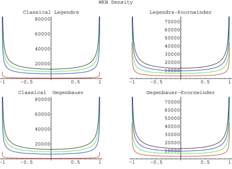
= 0.

WKB Density

-1 -0.5 0.5 1

Classical Gegenbauer

20000 40000 60000 80000

-1 -0.5 0.5 1

Gegenbauer-Koornwinder

10000 20000 30000 40000 50000 60000 70000

-1 -0.5 0.5 1

Classical Legendre

20000 40000 60000 80000

-1 -0.5 0.5 1

Legendre-Koornwinder

10000 20000 30000 40000 50000 60000 70000

Figure 2: WKB density of zeros of the

G

;A_{n (}

_x

_).

In this case the expression is very large and we will provide only the limit case when

A

!0. In this case we recover the classical expression [31], [32] wkb(x) =

p

2 + 16m2+ 4+ 16m+x2 16m2x2 16mx2 42x2

2(1 x2) :

For Legendre generalized polynomials we have, asymptotically,

asymp_wkb (

x

) =

p

R

asymp₍

_x

₎

(1

x

) (1 +

x

) (1

x

2+

mx

2 4

m

2

x

2+ 4

m

3

x

2)

;

where

Rasymp_{(x) = 7 8m+ 4m}2 12x2+ 2mx2 8m2x2 16m3x2+ 64m4x2 32m5x2+

+7x4+ 7mx4+ 6m2x4+ 44m3x4 112m4x4+ 80m5x4 96m6x4+ 64m7x4

2x6 10m2x6 4m3x6+ 16m4x6 32m5x6+ 96m6x6 64m7x6:

In Figure 2 we represent the WKB density of zeros for our generalized Gegenbauer polynomials. Notice that the value of the mass doesn't play a crucial role, since for

n >>

1,

W

m 1 2m

2, independently of

A

. We have plotted the Density function for dierent values

of the degree of the polynomials (from top to bottom)

n

= 210 4

;

1

:

5

10

4

;

104

;

103 for

two dierent cases: the generalized Legendre polynomials (

= 1

2) and the generalized

Gegenbauer with

= 5.

5.2.3 Numerical Experiments.

by computing the quantity

N

=Z 1 10

1 10

(

x

)

dx

Z 1

10 1 10

wkb(

x

)

dx;

which gives us (approximately) the number of zeros on such an interval. The result of such a calculation for the Legendre

L

A

2m(

x

) and Hermite

H

A

2m(

x

) families is given in table

1.

Table 1.

The number of zeros in [ 1 10

;

1

10] of the

L

A

2m(

x

) and

H

A

2m(

x

) polynomials.

2

m

L

2m(

x

)

L

A

2m(

x

)

H

2m(

x

)

H

A

2m(

x

)

100000 12753.7 12753.8 40.2634 38.8898 200000 25507.5 25507.5 56.941 55.4299 300000 38261.2 38261.2 69.7382 68.047 400000 51014.9 51014.9 80.5268 78.6623 500000 63768.6 63768.7 90.0317 88.0054 600000 76522.3 76522.4 98.6247 96.4471 700000 89276. 89276.1 106.527 104.207 800000 102030. 102030. 113.882 111.428 900000 114783. 114784. 120.79 118.208 1000000 127537. 127537 127.324 124.62

ACKNOWLEDGEMENTS

The research of the authors was supported by Direccion General de Investigacion Cientca y Tecnica (DGICYT) of Spain under grant PB 93-0228-C02-01. The authors thank to the referee for its useful suggestions and remarks and also for pointing out references [27] and [33].

References

[1] M. Abramowitz and I. Stegun Editors:

Handbook of Mathematical Functions.

Dover Publications, Inc., New York, 1972.

[2] R. Alvarez-Nodarse and F. Marcellan: A generalization of the classical Laguerre polynomials. Rend. Circ. Mat. Palermo. Serie II,

44

, (1995), 315-329.

[4] R. Alvarez-Nodarse and F. Marcellan: The limit relations between generalized orthog-onal polynomials. Indag. Math. (1997) (in press)

[5] E.R. Arriola, A. Zarzo, and J.S. Dehesa: Spectral Properties of the biconuent Heun dierential equation. J. Comput. Appl. Math.

37

(1991), 161-169.

[6] E. Buenda, S. J. Dehesa, and F. J. Galvez: The distribution of the zeros of the polynomial eigenfunctions of ordinary dierential operators of arbitrary order. In

Orthogonal Polynomials and their Applications.

M.Alfaro et al. Eds. Lecture Notes in Mathematics.

Vol. 1329

, Springer-Verlag, Berlin, 1988, 222-235.

[7] T. S. Chihara: Orthogonal polynomials and measures with end point masses. Rocky Mount. J. of Math.

15

(3), (1985), 705-719.

[8] T. S. Chihara:

An introduction to orthogonal polynomials.

Gordon and Breach. New York. 1978.

[9] N. Dradi: Sur l'adjonction de deux masses de Dirac a une forme lineaire reguliere quelconque. These Doctorat de l'Universite Pierre et Marie Curie. Paris, 1990. [10] N. Dradi and P. Maroni: Sur l'adjonction de deux masses de Dirac a une

forme reguliere quelconque. In

Polinomios ortogonales y sus aplicaciones.

A. Cachafeiro and E. Godoy Eds. Actas del V Simposium. Universidad de Santiago. Vigo 1988, 83-90.

[11] A. Erdelyi, A. Magnus, F. Oberhettinger and F. Tricomi:

Higher Transcendental

Functions.

McGraw-Hill Book Co. New York,

Vol 2

, 1953.

[12] J. Koekoek and R. Koekoek : On a dierential equation for Koornwinder's generalized Laguerre polynomials. Proc. Amer. Math. Soc.

112

, (1991), 1045-1054.

[13] R. Koekoek and H. G. Meijer: A generalization of Laguerre polynomials. SIAM J. Math. Anal.

24

(3), (1993), 768-782.

[14] R. Koekoek: Koornwinder's Laguerre Polynomials. Delft Progress Report.

12

, (1988), 393-404.

[15] R. Koekoek: Generalizations of the classical Laguerre Polynomials and some q-analogues. Thesis, Delft University of Technology. 1990.

[16] R.Koekoek: Dierential equations for symmetric generalized ultraspherical polynomi-als. Transact. of the Amer. Math. Soc.

345

, (1994), 47-72.

[17] T. H. Koornwinder: Orthogonal polynomials with weight function (1

x

)_{(1 +}

_x

₎

+

M

(

x

+ 1) +

N

(

x

1). Canad. Math. Bull.

27

(2), (1984), 205-214.

[18] A. M. Krall: Orthogonal Polynomials satisfying fourth order dierential equations. Proc. Roy. Soc. Edinburgh,

87

, (1981), 271-288.

[19] H. L. Krall: On Orthogonal Polynomials satisfying a certain fourth order dierential equation. The Pennsylvania State College Bulletin,

6

, (1940), 1-24.

[21] F. Marcellan and P. Maroni: Sur l'adjonction d'une masse de Dirac a une forme reguliere et semi-classique.Ann. Mat. Pura ed Appl.

IV

, CLXII, (1992), 1-22. [22] F. Marcellan and A. Ronveaux: Dierential equations for classical type orthogonal

polynomials. Canad. Math. Bull.

32

, (4), (1989), 404-411.

[23] P. Nevai: Orthogonal Polynomials. Memoirs of the Amer. Math. Soc.

213

, Providence, Rhode Island, 1979.

[24] A.F. Nikiforov and V. B. Uvarov:

Special Functions of Mathematical Physics.

Birkhauser Verlag, Basel, 1988.

[25] E.D. Rainville:

Special Functions.

Chelsea Publishing Company, New York, 1971. [26] J. Riordan:

An Introduction to Combinatorial Analysis.

Wiley, New York,

1958.

[27] A. Ronveaux, A. Zarzo, and E. Godoy: Fourth-order dierential equations satised by the generalized co-recursive of all classical orthogonal polynomials. A study of their distribution of zeros. J. Comput. Appl. Math.

59

(1995), 295-328.

[28] G. Szego:

Orthogonal Polynomials.

Amer. Math. Soc. Colloq. Publ.,

23

, Amer. Math. Soc., Providence, Rhode Island, 1975 (4th edition).

[29] W. Van Assche:

Asymptotics for Orthogonal Polynomials.

Lecture Notes in Mathematics

Vol. 1265

. Springer-Verlag, Berlin, 1987.

[30] S.Wolfram:

Mathematica. A system for doing Mathematics by Computer.

Addison-Wesley Publishing Co., New York, 1991.

[31] A.Zarzo and J.S. Dehesa: Spectral Properties of solutions of hypergeometric-type dif-ferential equations. J.Comput.Appl.Math.

50

(1994), 613-623.

[32] A.Zarzo, J.S. Dehesa, and R.J. Ya~nez: Distribution of zeros of Gauss and Kummer hypergeometric functions: A semiclassical approach. Annals Numer. Math.

2

(1995) 457-472.