Monterrey, Nuevo León a
INSTITUTO TECNOLÓGICO Y DE ESTUDIOS SUPERIORES DE MONTERREY
PRESENTE.-Por medio de la presente hago constar que soy autor y titular de la obra denominada
, en los sucesivo LA OBRA, en virtud de lo cual autorizo a el Instituto Tecnológico y de, Estudios Superiores de Monterrey (EL INSTITUTO) para que efectúe la divulgación, publicación, comunicación pública, distribución, distribución pública y reproducción, así como la digitalización de la misma, con fines académicos o propios al objeto de EL INSTITUTO, dentro del círculo de la comunidad del Tecnológico de Monterrey.
El Instituto se compromete a respetar en todo momento mi autoría y a otorgarme el crédito correspondiente en todas las actividades mencionadas anteriormente de la obra.
Characterization of the Stress-Softening and Permanent Set
Effects of Elastomeric Materials-Edición Única
Title Characterization of the Stress-Softening and Permanent Set Effects of Elastomeric Materials-Edición Única
Authors Victor Calva Mendoza
Affiliation Tecnológico de Monterrey, Campus Monterrey
Issue Date 2008-12-01
Item type Tesis
Rights Open Access
Downloaded 19-Jan-2017 02:55:02
INSTITUTO TECNOLÓGICO Y DE ESTUDIOS SUPERIORES
DE MONTERREY
CAMPUS MONTERREY
DIVISIÓN DE INGENIERÍA Y ARQUITECTURA
PROGRAMA DE GRADUADOS EN INGENIERÍA
CHARACTERIZATION OF THE STRESS-SOFTENING AND PERMANENT SET EFFECTS OF ELASTOMERIC MATERIALS
TESIS
PRESENTADA COMO REQUISITO PARCIAL PARA OBTENER EL GRADO ACADÉMICO DE:
MAESTRO EN CIENCIAS CON ESPECIALIDAD EN SISTEMAS DE MANUFACTURA
POR:
VICTOR CALVA MENDOZA
INSTITUTO TECNOLÓGICO Y DE ESTUDIOS SUPERIORES
DE MONTERREY
CAMPUS MONTERREY
DIVISIÓN DE INGENIERÍA Y ARQUITECTURA
PROGRAMA DE GRADUADOS EN INGENIERÍA
Los miembros del Comité de Tesis recomendamos que la presente Tesis del Ing. Victor
Calva Mendoza sea aceptada como requisito parcial para obtener el grado académico
de Maestro en Ciencias con especialidad en:
SISTEMAS DE MANUFACTURA
Comité de Tesis
__________________________________ Dr. Alex Elías Zúñiga
Asesor
____________________________ _________________________ Dr. Ciro Ángel Rodríguez González Dr. Héctor Rafael Siller Carrillo
Co-Asesor Sinodal
APROBADO
_________________________ Dr. Joaquín Acevedo Mascarúa
Abstract
In this work, the application of a phenomenological constitutive model able to predict
residual strains of isotropic, incompressible hyperelastic rubberlike materials is studied.
It consists in a form of the strain energy which accounts for the microstructural damage
developed during loading and unloading deformation process. Along with the study of
the application of the model, two new strain energy damage functions are proposed; the
first one is based on an exponential form that depends in a single material parameter to
predict the inelastic behavior of rubberlike materials; the second one is a simple function
with two fitting positive constants that characterize residual strain. Theoretical models for
the representation of uniaxial and equibiaxial extension are presented using
non-Gaussian constitutive models affected by a phenomenological function to account for the
Mullins effect. Also a comparison of the derived models with experimental data of
different materials is presented.
Also, an experimental set up has been designed to obtain data for equibiaxial
deformation state membrane inflation. the test consists in monitoring the evolution of a
rubberlike material membrane as inflated by steps of uniform static pressure. A
non-contact measuring system is used to obtain the stretch information from the material for
each inflation step.
At the end of the present work, we discuss the nanomanufacturing process of
thermosetting panels reinforced with carbon fibers and carbon nanotubes used in the lab
facilities of the Mechanical Engineering and Materials Science (MEMS) at Rice
University. A review of the main processing stages, the generation of the nanotubes, the
purification process, separation, embedding them into the composite, as well as the
technology and methodology employed for the qualitative characterization of the
different processing steps of the material was carried out. Finally, a description of the
Vacuum Assisted Resin Transfer Molding process is presented; it is the method
currently employed in the facilities of the MEMS department for manufacturing polymeric
Acknowledgements
I am grateful to my advisor Dr. Alex Elías Zúñiga for the opportunity to work with him and
for his guidance during the development of this work.
Thanks to the members of my Thesis Committee Dr. Ciro Rodriguez, and Dr. Hector
Siller for the support and help during my studies and their helpful input in this work.
Thanks to Dr. Enrique V. Barrera at Rice University for the opportunity to work in the
Mechanical Engineering and Material Science Department making possible the
conclusion of this research project.
Thanks to Ana Laura Jáuregui, José Luis González, René Ktnwa Córdoba, Gloria
López, Beatriz Montoya, Araceli Rivera, Arturo Marban, Ángel González, and Samantha
Rodriguez for their help, joy and cheers.
This work was carried out thanks to the support of the Research Chairs of Materials and
Nanotechnology and of Intelligent Machines of the Instituto Tecnológico y de Estudios
Superiores de Monterrey, Campus Monterrey, and also, of the CONACYT project:
Synthesis and constitutive modeling of biocompatible polymers for micro fluidic devices
Table of Contents
ABSTRACT... 3
TABLE OF CON TEN TS... 6
N OMEN CLATURE... 8
LI ST OF FI GURES... 11
LI ST OF TABLES... 13
OBJECTI VES... 14
I . I N TRODUCTI ON... 16
1.1 FUNDAMENTALS... 16
1.1.1 Therm oplast ic polym ers... 17
1.1.2 Therm oset t ing polym ers... 18
1.1.3 Elast om ers... 19
1.4 APPLI CATI ONS OVERVI EW... 23
1.4.1 Aerospace applicat ions... 23
1.4.2 Aut om ot ive applicat ions... 24
1.4.3 Medical applicat ions... 25
1.4.4 St ruct ural applicat ions... 26
1.4.5 Microelect ronic m echanical devices... 26
1.4.6 Nanocom posit es and sm art elast om ers... 27
I I . PRELI MI N ARI ES... 29
2.1 THE ELASTOMER MOLECULAR CONSTI TUTI ON AND MATERI AL ASSUMPTI ONS... 29
2.2 MECHANI CAL RESPONSE... 29
2.3 STATI STI CAL MECHANI CS... 31
2.4 AVERAGE STRETCH FULL NETWORK MODEL... 41
2.5 PHENOMENOLOGI CAL MODELS... 44
2.5.1 Ogden m odel... 44
2.6 MULLI NS EFFECT... 45
2.6.1 St rain int ensit y dam age m odel... 45
2.6.2 Ogden pseudo- elast icit y t heory... 47
I I I . MATERI AL CHARACTERI ZATI ON... 50
3.2 EQUI BI AXI AL EXTENSI ON – MEMBRANE I NFLATI ON... 52
I V. CHARACTERI ZATI ON OF MULLI N S AN D RESI DUAL STRAI N EFFECTS... 54
4.1 STRAI N ENERGY FUNCTI ON MODI FI CATI ON... 54
4.1.1 Model A.... 55
4.1.2 Model B.... 57
V. RESULTS AN D DI SCUSSI ON... 60
5.1 TRANSVERSE VI BRATI ON... 61
5.2 EQUI BI AXI AL TESTI NG... 68
VI . POLYMERI C N AN OCOMPOSI TE CHARACTERI ZATI ON... 73
CON CLUSI ON S AN D RECOMMEN DATI ON S... 78
APPEN DI X A. EXPERI MEN TATI ON METHODOLOGY... 80
APPEN DI X B. MEMBRAN E I N FLATI ON LAB MAN UAL: CARACTERI ZACI ÓN EXPERI MEN TAL DE ELASTÓMEROS... 87
APPEN DI X C. CARBON FI BERS- THERMOSETTI N G COMPOSI TE PAN ELS W I TH CARBON N AN OTUBE REI N FORCI N G MAN UFACTURE TECHN OLOGI ES... 101
Nomenclature
A Helmholtz free energy
B
Left Cauchy-Green deformation tensorF
Deformation gradient tensorF
, fi Tensile forcesG Gibbs free energy
I
Identity matrix3 2 1
,
I
,
I
I
Right or left Cauchy-Green deformation tensor invariantsJ Jacobian
L
Parallelepipedx
-axis side lengthM
Maximum strain intensityc
M Chain density
P Working pressure
0
R Undeformed membrane radius
S
Conformational entropyT Cauchy stress tensor
k j i
T
T
T
,
,
Principal Cauchy stress tensor componentss
T Cauchy stress accounting for permanent set
U Internal energy
W Strain energy per unit of volume
s
Wˆ Damage mechanism function
a Cord sectional area
b
Softening parameterc Permanent set related material parameter
* 0,c
c Convenient constants
f Normalized string frequency
i
s
f Softened string normalized frequency
k Boltzmann constant
i
l
Random flight step vectori
l
Random flight step vector magnitudel Cord length
m Strain intensity
o
m
Material constantn Material parameter
p
Arbitrary hydrostatic pressure( )
rip End to end configuration probability distribution function
r End to end distance vector
r Average end to end distance vector
0
r Undistorted chain end to end distance
o
r
Material constantch
r Current chain end to end distance
m
r Fully extended chain end to end distance
s Single chain entropy
0
t Undeformed membrane thickness
w Strain energy per chain
Θ Absolute temperature
(
η,Wm)
Φ Damage function
m
α
Ogden model material constantβ
Inverse of the Langevin functionη
Damage parameter3 2 1,λ ,λ
λ Stretches in the principal directions
ch
λ
Chain stretchm
ps
λ Permanent set in terms of the stretch
r
λ
Relative stretch0
μ
Shear modulus in the undeformed statem
μ
Ogden model material constant( )
I1μ Shear response function
v Virgin string frequency
s
v Softened string frequency
a
ξ Damage variables
ρ Material density
τ
Cauchy stress-softened tensor( )
ηφ ,φ
( )
ξa Damage functions1 1,ℵ−
List of Figures
Figure 1. Mullins effect schematization... 22
Figure 2. Entangled macromolecules lightly cross-linked forming an elastomeric 3D-network. ... 29
Figure 3. Undeformed chain conformation and total displacement vector. ... 34
Figure 4. Inverse of the Langevin function... 40
Figure 5. Arruda Boyce eight-chain configuration... 43
Figure 6. Transverse vibration experimental set up... 50
Figure 7. Pole membrane element subjected to equibiaxial stress... 53
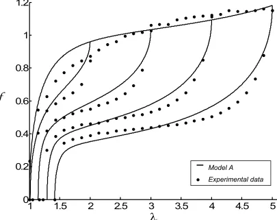
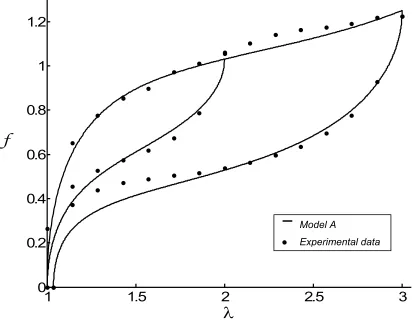
Figure 8. Frequency-stretch data for nitrile rubber string and normalized frequency curves accounting for stress softening and permanent set. Model A. with b = 0.4377, N = 20.893, c = 31.72, μ0 = 1.25 x10⁵ N/m2. ... 61
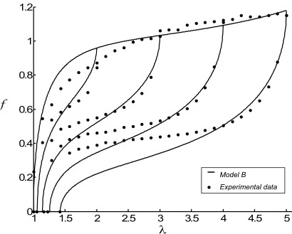
Figure 9. Frequency-stretch data for nitrile string and normalized frequency curves accounting for stress softening and permanent set. Model B. with b = 0.475, N = 20.893, c = 18, μ0 = 1.25 x10⁵ N/m2, n = 1.5. ... 62
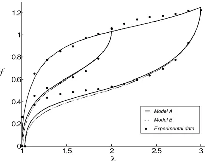
Figure 10. Comparison of constitutive models for nitrile rubber string and the experimental frequency data accounting for stress softening and permanent set. Model A. shown in continuous line, Model B. in hidden line, and experimental data in filled dots. ... 64
Figure 11. Frequency-stretch data for silicone rubber string and normalized frequency curves accounting for stress softening and permanent set. Model A. with b = 0.536, N = 6.31, c = 24.43, μ0 =1.39 x 10⁵ N/m2. ... 65
Figure 12. Frequency-stretch data for silicone string and normalized frequency curves accounting for stress softening and permanent set. Model B. with b = 0.6, N = 6.31, c = 149, μ0 =1.39 x 10⁵ N/m2, n = 2. ... 66
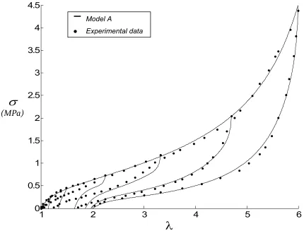
Figure 14. Equibiaxial engineering stress as a function of the equibiaxial stretch for
BALL9 from Johnson and Beatty. Model A. with μ0 = 0.3118 MPa, N = 34.25, b = 0.208,
c = 11.358... 68
Figure 15. Equibiaxial engineering stress as a function of the equibiaxial stretch for BALL9 from Johnson and Beatty. Model B. with μ0 = 0.3118 MPa, N = 34.25, b = 0.208, c = 17.18, n = 1.313... 69
Figure 16. Equibiaxial engineering stress as a function of the equibiaxial stretch for BALL10 from Johnson and Beatty. Model A. with μ0 = 0.1979 MPa, N = 34.25, b = 0.208, c = 11.358... 70
Figure 17. Equibiaxial engineering stress as a function of the equibiaxial stretch for BALL10 from Johnson and Beatty. Model B. with μ0 = 0.1979 MPa, N = 34.7, b = 0.1635, c = 19.13, n = 1.69... 71
Figure 18. Simple tension engineering stress as a function of the strain for polyethyleneand embedded nanotube system, (taken from Mokashi et al. [ 62]). ... 74
Figure 19. Modulus of a SWNT/LaRC-SI composite material vs. nanotube length for a 1% nanotube volume fraction, (taken from Odegart et al [ 61]). ... 76
Figure 20. Sketch of the transverse vibration - uniaxial stretching device. ... 80
Figure 21. Transverse vibration experimental set up... 81
Figure 22. Membrane inflation pneumatic circuit. ... 83
Figure 23. Inflation cylinder... 84
Figure 24. Reference marks in a membrane sample. ... 85
Figure 25. Inflated membrane contour and geometry... 86
Figure 26. SEM image of bundled HiPco nanotubes. ... 111
Figure 27. Typical TGA curve for HiPco nanotubes with iron impurities. ... 113
Figure 28. Typical Raman curve for HiPco nanotubes with iron impurities. ... 114
Figure 29. Schematic set up of the epoxy/carbon fibers panel preparation process.... 117
Figure 30. Carbon fiber fabrics after spraying carbon nanotubes in solution with a solvent. ... 118
Figure 31. Components of the vacuum bag for VARTM process... 120
Figure 32. Installed components for the VARTM process. ... 120
List of Tables
Table 1. St ress soft ening const it ut ive m odels lit erat ure review ... 23
Table 2. Residual st rain dat a com parison for nit rile rubber cord t ransverse
vibrat ion experim ent al analysis... 63
Table 3. Residual st rain dat a com parison for silicone rubber cord t ransverse
vibrat ion experim ent al analysis... 67
Table 4. Euclidean lengt h of t he error vect or for BALL9 and BALL10 unloading
Objectives
This work centers its attention into three main objectives,
the development of a constitutive model for rubber like materials which accounts for
stress softening with permanent set;
the design and assemble of an experimental set up for equibiaxial extension
elastomeric membranes testing;
a review of the state of the art of the preparation of polymeric nanocomposites and
their advantages over typical engineering materials.
The first part is focused in the development of a constitutive model to predict the elastic
and inelastic behavior of elastomeric materials including the effects of stress softening
and residual strains.
Along with the mathematical modeling of the mechanical behavior of rubberlike
materials, experimental protocols are needed to qualitative characterize elastomeric
materials, and also to verify the effectiveness of the models developed. Since the design
of experimental set ups to obtain data from rubberlike materials is one of the main
objectives of the present work, we work in the design and construction of an
experimental set up to measure equibiaxial stresses, and we discuss the application of
the set up to characterize uniaxial extension using small amplitude transverse vibrations of a rubber cord used in [ 1, 2, 3], to obtain residual strain data from different elastomeric
materials.
The design, construction and tuning of a set up able to generate equibiaxial extension
experimental data, is required to test rubberlike membranes of different compositions
and sizes; versatility and adaptability for different testing conditions, e.g. pressure range
and temperature, are required. Among different testing devices that have been used to
analyze elastomers under equibiaxial conditions, a feasible set up considering the
The final goal of this work involves the study of nanostructured materials as
reinforcements of elastomeric matrices. The preparation of polymeric nanocomposites
and the effect of this kind of structures when embedded into a polymeric network will be
reviewed. Additionally, we would intend to connect non-Gaussian statistical molecular
theory to characterize nanocomposite polymers such as PMMA, PDMS, and COC,
I. Introduction
Enormous efforts around the world have been taking place to understand and
mathematically express the complex mechanical behavior of the different types of
polymers, which are, day by day more often used in highly specialized engineering
applications. As their use increase, more reliable and realistic constitutive models are
required to simulate and predict their performance for a given application. The relevance
in generating more accurate ways to predict the performance of this kind of materials
becomes evident in areas such as mechanical design methodologies, manufacturing
and electronics, etc., as well as the repercussion in nearly every industry and common
life applications. Polymers can be natural or synthetic, organic or inorganic, branched or
not, each of them comprises a wide variety of structures with different mechanical,
chemical, electrical, thermal properties, reason why it is easy to find these materials as
applications in any kind of task everywhere.
1.1 Fundamentals
By polymer we understand a group of macromolecules entangled with each other and
joined together by either primary or secondary bonds depending on its type; each
macromolecule has a chain-like structure formed by a group of smaller entities called
monomers, these are joined together one another by primary chemical bonds created by a process called polymerization [ 9].
Polymerization is the process by which the short unit called monomer or a group of few
of these units called oligomers can become one long linear chain by means of covalent
bonding. In terms of the mechanism of polymerization there are two basic types of
polymerization, step-growth polymerization and chain-growth polymerization. The main characteristic of the first type is that all molecular species in the system can react with
each other to form higher molecular weight species; in the chain growth polymerization
the chain growth occurs only by addition of monomer to reactive sites present on the
A fundamental classification of polymers according to their structure, and mechanical
and thermal behavior establishes three mayor categories: thermoplastic polymers, thermosetting polymers and elastomers.
1.1.1 Thermoplastic polymers
Thermoplastic polymers are made of long macromolecules joined with each other by
weak van der Waals bonds, characteristic that causes ductile behavior. Thermoplastics
might be branched to form bulk structures with lower density than the un-branched type,
as density in the molecular chain reduces the strength of the material and the stiffness
reduce as well. Thermoplastics structure is composed partially by crystalline and
partially by amorphous molecular configuration; their long molecules can be untangled
upon the application of a stress allowing them to arrange a parallel string group forming
a crystalline region. Other way to induce this kind of molecular conformation is by
subjecting the material to slow cooling, inducing the molecules to fold and align forming
packs of crystalline sectors that contribute to strength and rigidity.
An important characteristic of thermoplastics is that they can be melted, shaped and
solidified again, once and again. This allows this kind of materials to be recycled.
Thermoplastics behavior depends to a great extent in its temperature, this phenomenon
can be clearly seen in the change of the modulus of elasticity as a response in a change
on the temperature; there are three temperature ranges dividing the thermoplastic
behavior, divided by, Tg, the glass temperature, and Tm, the melting temperature, where the thermoplastics properties change rate increases (or decreases). In liquid state, i.e.,
above the melting temperature, the polymer strength is nearly zero. The chains in the
material are separated from each other with weak secondary bonding between them
thus, making easy for them to move and slip from their original places and rearrange
without resistance. This condition makes the thermoplastics suitable for the different
When the temperature is below the melting point, the secondary bonds become
stronger, thus, the strength and rigidity of the bulk increase and an elastic and plastic
behavior is observed. Crystalline, semicrystalline or amorphous structures may be
achieved depending on the flexibility of the polymer’s chain and the thermal processes.
The first type has higher chain density and because of that the bonds between them are
stronger, this structure has the largest modulus of elasticity, although they are always
amorphous transition zones remaining in these thermoplastics. The amorphous kind
behaves more as rubber, resilient and ductile. Semicrystalline thermoplastics are a
combination of both of them, they have intermediate density with packs of crystalline
molecules among amorphous ones, and their properties are as well, between the ones
of the crystalline and amorphous polymers.
The lowest limit that changes dramatically the thermoplastic’s properties is the glass
temperature; below this temperature the material has high strength and stiffness,
although it becomes fragile. Crystalline thermoplastics do not have glass transition
temperature; they behave in a crystalline way above the melting point. Semicrystalline
ones do observe a change in properties change rate below this point but the most
affected are the amorphous polymers. As the side groups in a thermoplastic become
more complex, the glass temperature tends to be higher.
1.1.2 Thermosetting polymers
As the thermoplastics, they are composed of large molecules which may have branches
or not, but in this case, these chains have a large number of intersections joining them
called crosslinks; in other words the thermosetting polymers structure is three
dimensional network with entangled long linear molecules united by strong primary
bonding in certain points along them.
The crosslinks may be simply formed by a union between two chains in the network or
As the primary bonds cannot be dissolved as temperature rises the thermosetting
polymers remain solid at high temperatures. If the temperature exceeds the degradation
temperature thermosets simply char without loosing their rigidity and strength to great
extent. This characteristic makes this type of polymers non-recyclable.
The crosslinkings make the chains in the thermosets remain in their place without
relative displacements reason why these kind of polymers exhibit high strength, stiffness
and hardness. For the same reason they are low resilient and are as ductile as the strain
of the chains between crosslinks, in addition to the one of the covalent bonds in the
network, allows.
1.1.3 Elastomers
Elastomers are a kind of polymer whose fundamental characteristic is that they can be
stretched several times their original length and then recover the original form when
unstressed; thus, natural or synthetic polymers exhibiting this kind of behavior are called
rubberlike solids.
Elastic deformations above 200% are reached with elastomers because of their
particular molecular structure. They are constituted by long flexible chains joined
together by secondary bonds and, in certain places, by cross-links, which connect chain
to chain generating a 3D molecular network; as force is applied to an elastomer, the
intertwined chains tend to untangle and align as long as the cross-links allow them to,
this deformation is much grater than that of thermosets because of the small quantity of
cross-links in elastomeric networks; as load continues increasing, the strain of the
primary bondings adds to the first one to reach the furthermost elastic deformation.
Thus, the molecular state of the material changes according to the loading and, by
consequence, the elastic module.
components on a single macromolecular chain [10]. In these, one of the phases has
glass transition temperature above its service temperature and, because of that, it
behaves in a crystalline manner, these segments in the macromolecule form bonds with
their own type in other molecules generating crystalline domains acting strong and stiff
generating physical crosslinks. The second and dominant phase in the macromolecule
has lower glass transition temperature and then behaves in a rubbery way enabling
large recoverable strains.
The elastomeric matrix is composed primarily by an amorphous linked polymer chains
network. These links between them might be conformed by either physical or chemical
crosslinks. Physical linking can be formed by small crystalline domains, absorption of
chains onto the surface of finely divided particulate fillers, coalescence of ionic centers
or coalescence of ionic blocks. Chemical linking is created from random connecting
segments of complete chains, random copolymerization or endlinking of functionally
terminated chains, which is the most appropriate technique to form well defined
structures [10].
Rubber mechanical properties might be increased by addition of particles known as
fillers. Carbon black fillers help increasing tensile strength and tear resistance; they can
improve cut growth and fatigue resistance, reduce resilience and raise hysteretic
behavior, all depending in quantity and filler particle size. Silica fillers improve tensile
strength and reduce heat buildup. Other filler compounds as hydrous aluminum silicate,
potassium aluminum silicate, magnesium silicate, titanium dioxide and calcium
carbonate are often used.
Physical surrounding affect the elastomer degradation rate or even modifies the material
properties. Chemical compatibility with the service medium has to be verified because of
their capacity to absorb liquids and swell, react chemically generating changes in the
polymer structure, or allowing extraction of solubles causing a decrease in volume. The
thermal properties are essential as well; the mechanical properties will fluctuate along
differences in the degree of deterioration [11]. It is also known that rubbers exhibit
thermoelastic effects, i.e. a rubber sample subjected to a constant load contracts
(reversibly) on heating and gives out heat when stretched.
Low Young's modulus, high recoverability of strain and high extensibility are basic
mechanical characteristics of rubberlike solids [12]; they exhibit viscoelastic
characteristics such as creep, stress relaxation and stress recovery as well. Along with
these phenomena, their highly nonlinear behavior, stress softening and permanent set
effects have to be considered to evaluate the elastomer performance for a given
application.
Elastomers exhibit a stresssoftening effect known as Mullins effect, this is, the stress
required to elongate a virgin elastomer to a given length is higher than that required to
stretch it to the same length at subsequent loading cycles as long it remains below the
first maximum strain; if that strain is reached again, the new stress becomes equal than
the stress generated for the same previous deformation; for further extension the
material behaves as in the virgin state. If the material is unloaded for a second time, the
path changes again as described. This inelastic behavior was named after L. Mullins
(1947), although was first observed by Bouasse and Carriθre (1903) [13].
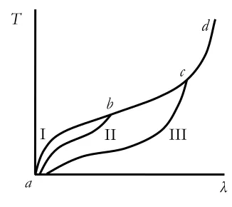
As stated in [12], the ideal loadingunloading path in simple tension is shown in figure 1;
stress T against stretch l is plotted to illustrate the Mullins effect. The material is first
stretched from a virgin state to an arbitrary length b through I, if the material is then
released, it would follow the return path II to a, on reloading, the latter path is followed
until the maximum stretch in b is reached again; for larger stretching the primary loading
path is taken over again from b to d, but if in an arbitrary point c, before d, the material is
The curves in figure 1 represent the loading/unloading typical simple tension behavior
without viscoelastic phenomena and strain rate dependency of a rubberlike material
exhibiting stress softening and permanent set.
d
c
b
a λ
II III
I
[image:24.612.224.387.173.318.2]T
Figure 1. Mullins effect schematization. Idealized loading/unloading curves for simple tension.
Mullins effect occurs in both, filled and unfilled rubbers, but fillers increase hysteresis in the material [ 12]. The stiffness lost in the loading cycle is recoverable partially or totally
in a period of time (usually long at room temperature), but might be greatly accelerated with an increase in temperature [ 13]. As Mullins noted, different magnitudes of softening
occur according to the stretch direction, softening magnitude is greater in the direction of
the greatest deformation of the material, and so, anisotropic stress-strain properties take place under stretching [ 12]
Related to the softening phenomena exhibited by elastomeric materials, residual strains
become evident after deformation, known in the rubber industry as permanent set. This
term refers to the difference in size of a virgin elastomeric element prior and after
deformation. Along with the softening effect, the virgin state is partially recovered in a
period of time.
Previous works on the characterization of the stress-softening and permanent set effects
works are classified by their approach, the inclusion or not of the permanent set effect,
and if so, the number of parameters necessary to model the inelastic behavior, where
the first number indicates the parameters required to model the virgin material loading
curve, and the second the parameters required for the unloading and reloading softened
[image:25.612.83.526.217.479.2]paths characterization.
Table 1. Stress-softening constitutive models literature review
Author Year Approach Accounts for
permanent set
Number of parameters
Holzapfel et al. [ 14] 1999 Phenomenological ● 6+1 Beatty and Krishnaswamy [ 15] 2000 Phenomenological
Bikard and Désoyer [ 14] 2001 Continuum damage
mechanics ●
5+12
Drosdov and Dorfmann [ 17] 2001 Physical ● 3+1 Zúñiga and Beatty [ 3] 2002 Phenomenological
Chagnon et al. [ 18] 2006 Physical
Dorfmann and Ogden [ 19] 2003 Phenomenological ● 6+3
Qi and Boyce [ 20] 2004 Phenomenological
2004 Physical Makovska and Kacianauskas
[ 21]
Diani et al. [ 22] 2005 Physical ● 2+1
Elías-Zúñiga and Calva 2008 Phenomenological ● 2+2
1.4 Applications
overview
Elastomeric materials are, day by day, covering more specialized and high responsibility
applications as the predictive mathematical models develop better and more time
efficient ways to simulate their mechanical behavior. Investigations, covering a wide
range of different applications, have been taking place in recent times to obtain as much
as possible of elastomers potential.
1.4.1 Aerospace applications
Different elastomeric materials are being used in aerospace applications due to the
solutions given the chemical inertness and thermal stability of the material; their high
resilience make them ideal as sealing elements. The importance of fully understanding
the behavior of the materials for these high responsibility applications becomes evident
as we remember that one of the main factors resulting in the Challenger space shuttle
explosion in 1986 was the failure of an elastomeric O-ring.
“In view of the findings, the Commission concluded that the cause of the Challenger accident was the failure of the pressure seal in the aft field joint of the right Solid Rocket Motor.”
This was the conclusion presented in the Report of the Presidential Commission on the Space Shuttle Challenger Accident [ 23], in which the partial responsibility of the
elastomeric element was found to be related to the temperature at launch time, which
was out of the recommended O-ring material working temperature range for the
particular application.
1.4.2 Automotive applications
Elastomers are being used nowadays to solve design and performance of different
automotive parts. Heat and chemical resistance, low permeability, long life, good
abrasion resistance, are characteristics of different elastomers that fit well as solutions to
many of the needs in vehicles design.
Apart from the use of rubber for tires, different systems in the engine require materials for service conditions were elastomeric materials can work adequately. In [ 24],
Hashimoto et al. described the conditions and requirements for different elastomer
elements working in; a gasoline engine, such as synchronous belts, seals and gaskets,
oil and air hoses, vibration isolators; the fuel and hydraulic system, the fuel hose, filler
neck hose, evaporation hose and control hose; the steering system, as the power
steering hose and the seals for this system; air conditioning system, hoses and seals; as
well as seals and diaphragms for the different systems in a vehicle. Elastomeric
fuels, oils and heat, their cold flexibility and sealing ability. The wide range of
applications and the fact that the service conditions in one is completely different to the
others requires the usage of different types of elastomer with specific mechanical
properties to function as desired in each given system. Tensile strength, elongation, the
dynamic complex modulus, dynamic permanent set, are significant mechanical
properties involved in the performance of the elements to be considered. Along with
these, thermal and aging properties as well as chemical resistances are important for
elastomer selection.
1.4.3 Medical applications
Need for precise mechanical characterization of elastomers becomes evident in
applications such as balloon angioplasty. This medical procedure allows blocked or
narrowed coronary arteries to restore blood flow, preventing heart failure alleviating the
stenosed artery by means of an inflated small balloon at the tip of a catheter. According
to Sauerteig and Giese [25], the elastomer membrane needs to be as thin as possible,
so as to produce a minimum deflated balloon profile, burst pressure of more than 15 bar
to dilate hard and heavily calcified stenosis and requires defined pressure and diameter
characteristics (balloon compliance). Low or noncompliant materials such as PET and
nylon are used for manufacturing this type of highpressure medical balloons [26]. A
critical variable involved in the performance of a balloon catheter is the bifurcation
pressure (internal pressure to initiate dilation), and subsequent uncontrolled inflation,
due to the highly nonlinear phenomenon [27]. Haridas and Haynes in [27], remark on the
need of effective hyperelastic materials characterization to be applied in nonlinear finite
element codes in both, uniaxial and biaxial stretching conditions for complete
understanding and control of these medical devices.
Different kinds of elastomers are being used to reproduce different biological soft tissues
to aid medical sciences replacing damaged body membranes. K.D. Kavlock et al. [28],
analyzed the poly(esterurethane urea)s suitability for musculoskeletal tissue
development. Since the early 1990's polyurethane elastomers have been studied for
and thus, insufficiency in blood pumping capability, condition that can be treated by
means of cell implantation with patches capable of coexistence with human organs, and
properties similar to those of the heart muscle that show nonlinear elasticity and
anisotropy [11]. The use of biocompatible elastomers to be used as patches in addition
to cultivated cells is being investigated to develop techniques of feasible and economic
implantations with low risk of rejection. Q. Z. Chen et al. [30] studied the physical
characteristics of poly(glycerol sebacate) elastomer and it's similarities with myocardial
tissues. L.A. Hidalgo Bastida et al. investigated poly(1,8octanediolcocitric acid)
elastomer and it's potential for cardiac tissue applications and found that it's porous
characteristics and adequate mechanical properties provides capability to serve as
scaffold for heart tissue regeneration techniques [31].
In addition to heart muscle regeneration elastomers have been investigated for
applications in medical sciences such as sutures, arteries or veins replacements,
jawbone, nose, ear, teeth, and tendon restoration and aesthetic plastic surgeries [32].
1.4.4 Structural applications
In any structural design appropriate material constants and properties are fundamental
to obtain effective results for a given application; passive vibration control and shock
absorption are important areas. As an example, in the design of thermoplastic elastomer
for railway paths (supports placed between the base of the steel rails and the pre
stressed concrete sleepers), high values of stiffness in the pads increases the dynamic
overloads to the nonsuspended masses, accelerating the deterioration of the railway,
while a low value leads to an excessive subsidence of the rail, increasing stresses [33].
1.4.5 Microelectronic mechanical devices
The improvement of microactuators is another area where elastomers are finding
important specialized applications. As applications for MEMS grow in number and
variety, devices as microactuators are required to be more efficient, low cost and easily
manufactured. In 1999 Khoo and Liu [34], presented a microfabricated, membrane type
magnetic actuator; employing magnetic electroplated Permalloy pieces, embedded on a
robust, biocompatible system. In 2004 Hung et al. designed and proved electrical
connections though microfabricated suspensions on a circular tunable elastomeric
membrane actuated by pressurized air [35]. Important investigations have been taking
place in the development of dielectric elastomers, materials capable of achieve large
strains able to transform electric energy into mechanical work. In 2005, P. Dubois et al.
[36] reported the fabrication and testing of a micromachined metallic ion implanted
dielectric electroactive polymer diaphragm actuator, system that can be employed by
complex structures such as robotic arms, grippers and orientating devices or used
directly to interact with liquids, gases or even human body [36]. J. S. Plante and S.
Dubowsky discussed the need for more accurate models to describe the deformation
obtained from the application of voltage difference across the elastomeric film of
dielectric elastomer actuators [37]. The fact that the behavior of these materials is still
not completely understood limits the selection of this kind of devices for high
performance applications. High strains in the membrane make Hookean models such
inadequate. Hyperelastic models function well for constant stretch rates but cannot
describe the viscoelastic behavior of the film. More complex models such as Mooney
Rivlin with Maxwell viscosity and finite element with quasilinear viscosity agreed well
with short strains but failed to describe large stretches of up to 5.0, generated by these
devices. In the article, a modified BergströmBoyce model was used to predict
experimental data reporting good agreement with the observed behavior.
1.4.6 Nanocomposites and smart elastomers
Recent studies have been focused in the development of elastomeric materials
reinforced with nanotubes or nanoparticles. Several rubber matrices such as natural
rubber, synthetic polyisoprene, styrenebutadiene, butyl rubber, polybutadiene, ethylene
propylene, silicone and nitrile rubbers have been investigated as hosts for clay
nanocomposites. Increase of stiffness and strength with minimal ductility and impact
resistance loss, decrease of permeability and swelling in solvents, improvement in
abrasion, flame resistance and thermal endurance, enhancement in electrical
conductivity and optical properties, in relation to the single polymeric matrix, can be
techniques, such as melt intercalation used by Arroyo et al. require information on the
rheological behavior of the system, i.e. polymerpolymer and polymerfiller interaction,
as stated in [38]. Zhao et al. [39] have reported the improvement of tensile strength, high
dynamic mechanical loss values, and reasonably good stabilities in nitrile butadiene
rubber with addition of hindered phenol nanoparticles. Carbon nanotubes have been
studied as fillers to modify properties of elastomers as an alternative to common fillers or
nanoparticles, e.g. De Falco et al. [40] compared the properties of styrenebutadiene
rubber reinforced with multiwalled carbon nanotubes to carbon filled styrenebutadiene
rubber, reporting that employing multiwalled carbon nanotubes increase the mechanical
properties above those obtained by the addition of carbon black fillers.
Shape memory polymers are materials developing extensively in the last decades; these
materials are capable of shifting shape given an external stimulus to recover a
predefined form after being reshaped by means of a mechanical stress to a temporary
form [41]. This phenomenon is also present in elastomeric materials, and has been
gaining territory in different areas of applications such as vascular stents, orthodontic,
wires, vibration dampers, pipe couplings and actuators [42]. As an example, the work
presented in 2007 by Cai and Liu [42], where the shape memory effect of poly (glycerol
sebacate) elastomer was investigated. A shape memory ratio above 99.5% was
reported for this biodegradable and biocompatible elastomer, by means of thermal
stimuli. Other types of smart elastomeric material are the magnetorheological
elastomers; these are constituted by polarizable particles in a polymer medium and the
basic characteristic is that the material shear modulus is dependant of the applied
magnetic field within the preyield regime; due to this important characteristic
magnetorheological elastomers capability are being studied to be applied in areas of
vibration control, such as adaptive tuned vibration absorbers [43] or sandwich structural
II. Preliminaries
The statistical analysis and the thermodynamics involved in the mechanical behavior of
elastomers give way to the formulation of network models which successfully reproduce
the behavior of hyperelastic materials. These basic aspects of rubber-like material
theoretical modeling are the central topic of this chapter.
2.1 The elastomer molecular constitution and material assumptions
Hundreds or even thousands of monomers joined by strong chemical bonds constitute a
single flexible macromolecule of an elastomeric material. Many of these molecules,
entangled and interacting with each other by the effects of van der Waals forces
between them and joined together in specific places by chemical cross-links, form a 3D
network of an elastomeric material as shown in figure 2. This complex morphology
makes difficult to obtain stress-strain relations to predict the behavior given the intrinsic
phenomena in their nature. Several considerations have to be made in order to
approximate the mathematical models to the response of a physical system. The
analysis developed in the present work assumes hyperelasticity, incompressibility and
isotropic nature in the elastomeric materials.
Figure 2. Entangled macromolecules lightly cross-linked forming an elastomeric 3D-network.
2.2 Mechanical
response
When a continuum body is deformed from its undistorted state from which a defined
particle, with a position vector X coordinates (
i
position with a vector defined by , with coordinates x (
j
x j =1,2,3), the deformation gradient tensor F has coordinates
i j ij
F =∂x ∂X . The isochoric deformation in terms of
the principal stretches λ1,λ2,λ3 follows xi =λiXi (i =1,2,3
3
). The left Cauchy Green
deformation tensor is used in order to exclude the rotation of the body from the
calculations since it does not contributes to the stress state of the continuum, it is given
by B 2 3 2 2 2e λ λ + +
1 2
1e e
λ T
FF
B= = , (1)
where B is a symmetric tensor; its magnitude can be computed as m= B⋅B, called
strain intensity. In the reference configuration, as B=1, m= 3, and m> 3 for any deformation state.
An isotropic, incompressible, hyperelastic material is an ideally elastic material for which
the stress – stretch behavior can be determined by means of a strain energy function
; where stand for the invariants of B as,
(
1, 2, 3)
ˆˆ W I
W
W = λ λ λ =
(
I1, 2,I3)
,I3B
2 ,,I 1 I
I1=tr , (2)
( )
[
B2]
tr − B 2 1 2 2 1 I =
I , (3)
det
3 =
I . (4)
Furthermore, given the incompressibility condition, the Jacobian has the form
, and from the third invariant
1
det =
= F
J λ1λ2λ3 =1; the strain energy function is then a function of solely the first and second invariants of the left Cauchy Green deformation
tensor as W =Wˆ
(
λ1,λ2)
=Wˆ(
I1,I2)
.The relation between the strain energy function Wand the Cauchy stress tensor for
an incompressible, isotropic, hyperelastic material, is given by
(
)
(
)
1 2 1 1 2 11 , ,
− − ℵ + ℵ + −
= I B B
T p I I I I , (5)
for which p is an arbitrary pressure, and the response functions ℵ1
(
I1,I2)
, are given by(
1 21 I ,I
− ℵ
)
(
)
(
)
(
)
(
)
2 2 1 1 2 1 1 1 2 1 1 2 1 1 , ˆ 2 , ; , ˆ 2 , I I I W I I I I I W I I ∂ ∂ − = ℵ ∂ ∂ =ℵ − , (6)
and need to satisfy and , for all isochoric deformations of B
[3]; the latter equality holds when and only when , in equation (5).
(
1, 2)
01 >
ℵ I I ℵ−1
(
I1,I2)
≤00
1=
ℵ−
Alternatively the principal Cauchy stresses in terms of the principal stretches λ1,λ2,λ3, can be expressed as
i i i W p T λ λ ∂ ∂ + −
= ˆ ; i∈
{ }
1,2,3 , (7)where p stands for an arbitrary hydrostatic pressure.
Rubberlike materials, because of their complicated morphology and differences between
one another create a challenging problem for the definition of a strain energy function
that captures in great extent the way elastomers perform elastically. Different
approaches have been considered in order to develop an adequate model; the bases for
most of these theories are statistical analysis and thermodynamics theory, considering
the deformations of these materials as a purely entropic phenomenon. A review of this
analysis is shown in the next section.
2.3 Statistical
Mechanics
The nature of the carbon bonding, i.e. angle of 109.5° and rotational capabilities around
of possible chain conformations. In an elastomer, a chain is defined as the number of
segments in a macromolecule between two cross-links; this number of cross-links in a
polymer is related to the stiffness of the material. If a polymer with no cross-linking is
sufficiently stressed, the weak van der Waals forces holding the chains together will
allow slipping and untangling and the result would be large stretches given that there is
no rotation and moving restrictions for the chains; in a cross-linked polymer, if the same
force is applied, the cross-links would act as restrictors and the stretching capabilities
would be proportionally reduced to the cross-linking degree. Therefore the size of the
chains in the polymeric matrices is then an essential factor to consider in a stress stretch
relation.
2.3.1 Thermodynamics
As noted before, elastomers exhibit thermoelastic behavior resembling the behavior of
an ideal gas; this can be noticed as the pressure to contain a gas at a constant volume
will rise as the temperature is increased, for rubber the same effect is observed, the
necessary force to maintain a rubber sample stretched to a certain length is proportional
to the temperature of the material. The expressions used to model rubberlike structures
within this particular approach can be derived from the first and second laws of thermodynamics [ 45].
For a macroscopic elastomeric rectangular parallelepiped specimen placed in a
Cartesian reference system, with its sides aligned with the reference axes, the side
oriented in the
x
-axis has a lengthL
0, in an unperturbed state, andL
when a force in theF
x-th direction is applied, the following thermodynamic expressions relate the force, length, temperature , internal energy U , entropy , Gibbs and Helmholtz free
energies G and :
Θ S
A
FL S U
G = −Θ − , (8)
LdF Sd
dG=− Θ− , (9)
FdL Sd
Θ Θ Θ ⎟ ⎠ ⎞ ⎜ ⎝ ⎛ ∂ ∂ Θ − ⎟ ⎠ ⎞ ⎜ ⎝ ⎛ ∂ ∂ = ⎟ ⎠ ⎞ ⎜ ⎝ ⎛ ∂ ∂ = L S L U L A
F . (11)
Along with the Maxwell’s reciprocity relation,
, L F L S ⎟ ⎠ ⎞ ⎜ ⎝ ⎛ Θ ∂ ∂ − = ⎟ ⎠ ⎞ ⎜ ⎝ ⎛ ∂ ∂ Θ (12)
can be used to determine the force – extension relation in terms of the conformational
entropy of the elastomeric chain system as
Θ ⎟ ⎠ ⎞ ⎜ ⎝ ⎛ ∂ ∂ Θ − = L S
F , (13)
where the term considering change in internal energy is nearly zero since the
deformation is provided by chain untangling not by atom separation; thus, the term is
neglected in the derivation of (13).
2.3.2 The Freely Jointed Chain Model
Considering a freely jointed chain, which consists in a hypothetical linear chain with
equal segments and where the angle between them can assume any possible value, the
theory of random flight can be used to determine the mean end to end distance of the
chains constituting an elastomer. The number of possible conformations depends on the
distance between chain-ends, when they are as far as possible there is only one
conformation (straight chain), but for close distances in relation to the chain length, the
possible conformations grow in number. Thus, the conformational entropy of a single
chain is proportional to the number of conformations with the same end-to-end distance
[46]. Diverse statistical entropic analysis of an elastomer combined with basic
thermodynamic relations have been studied to generate convenient expressions relating
y
x
R
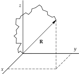
[image:36.612.237.376.74.204.2]z
Figure 3. Undeformed chain conformation and total displacement vector.
Considering a chain with one of the ends fixed in an origin where , and the other
end is localized at a distance defined by a vector , connected by randomly oriented
segments with the same length ; after steps the particle has traveled a distance 0 0 = r N r l N
∑
= = N i i 1 lr . (14)
The probability that the j-th segment will follow a jump vector
l
j, is given by the function( )
jj
p
l
; then, the average vector distance traveled is obtained by( )
∑
= = N i i i i p 1 l lr . (15)
The scalar distance traveled might be found by the average of the magnitude of the
vector , whose square is
r
∑
∑
= = ⋅ = ⋅ N j j N i i 1 1 l l rr . (16)
(
)
( ) , ... , 1 2 1 3 1 2 1 22
∑
∑
≠ = − ⋅ = + ⋅ + + ⋅ + ⋅ + = N j i j i j i N i i N N l Nl
r l l l l l l l l (17)
defining the scalar product in the last term, the average of the scalar distance is
∑
∑
≠ = ⋅ = N j i ij j i N ii ll
l
r cosθ
1 2
2 .
(18)
As the length of the segments is the same and, following the logic that for every possible
direction of a segment the probability to find a segment in the opposite direction is the
same, making the sum of both of them zero, the average of the cosine terms vanishes,
so equation (18) becomes
2 2
Nl
r = . (19)
Equation (19) is the resulting expression of the theory of free flight, representing the squared mean end to end distance of a polymeric chain [ 46].
Given the high extensibility of a polymeric chain, the deformation is generally expressed
as the relation between the current length of the mean end to end vector and the length
of the vector in its unstrained state as λch =rch r0 ; alternatively, the magnitude of current length of the mean end to end vector length, related to the length of the fully extended
chain vector rm = Nl, is called the relative chain stretch, this is
Nl r r r ch m ch r = =
λ . (20)
2.3.3 Entropy of a single chain
According to the principles of statistical thermodynamics [ 45], for a single chain the
( )
r p ks= ln . (21)
Upon deformation, the change in conformational entropy is
( )
( )
i i i r p r p k s * ln =Δ , (22)
where is the number of possible configurations for a chain with distance between
ends , in the undeformed state, and,
( )
ri pi
r
p( )
ri * represents the analogous probability for the deformed state; for the chains with initial length , the change in theconformational entropy becomes
i
N ri
∑
Δ = − i i io N s
S
S . (23)
2.3.4 Gaussian approximation
Assuming a Gaussian distribution as in [ 47], p
( )
r is given by(
x y z)
dxdydz b e ( )dxdydzp b2x2 y2 z2
2 3 3
,
, = − + +
π , (24)
where b2 =3 2Nl2, which represents the probability for the chain end to end distance vector r to end within the intervals of a cubic differential volume formed by the limits x
to x+dx, y to y+dy and to z z+dz. Noticing that the probability function is spherically
symmetrical, r2 =x2 + y2 +z2, then
( )
222 3 3 r b e b r
p = −
The resulting entropy would depend on the number of possible conformations for the
freely jointed chain with an end to end vector with ending within the limits of a differential
volume dv as
(
)
[
p x y z dv]
ks= ln , , , (26)
for a Gaussian distribution, since the natural logarithm of the volume element is a
constant, the entropy becomes
2 2
r kb c
s= − , (27)
where is an arbitrary constant. The entropy of deformation of a single chain with an
end to end distance with coordinates , in the unstrained state, and c
0
r x0,y0,z0 r with
coordinates x,y,z, after deformation to stretches in the principal directions λα =α α0, where α stands for x,y,z, becomes
(
2)
0 2 0 2 0 2 z y x kb c
s= − + + , (28)
for the unstressed state and
(
2)
0 2 2 0 2 2 0 2 2 z y x kb c
s= − λx +λy +λz , (29)
when deformed; thus, the chain contribution to the entropy of deformation of the full
network is
(
) (
) (
[
1 1 2 2 10 2 2 0 2 2 0
2 − + − + −
− =
−so kb x x y y z z
s λ λ λ
)
]
. (30)And the total entropy of deformation of the network can be computed by the summation
(
)
(
)
(
)
[
2]
0 2 2 0 2 2 0 2
2 1 1 1
z y
x kb
s
S=∑Δ =− x − ∑ + y − ∑ + z− ∑
Δ λ λ λ . (31)
The chain vectors have equally possible random directions; the summations of their
individual components result in one third the total displacement as,
0 r
∑
∑
∑
∑
2 ==0 = = 2 0 2 0 2
0 y z 1 3 r
x , where the latter summation is the same as the product
of the number of chains per unit volume , and the mean squared end to end
distance, yielding
c M
(
3)
3
1 2 2 2+ 2 + 2−
− =
ΔS Mckb r λx λy λz . (32)
Making the assumption that the length of the mean square chain vector in the unstrained
state is the same as for a corresponding set of free chains, this is r2 =3
( )
2b2 , the total entropy of deformation can be expressed as(
3)
2
1 2 + 2 + 2−
− =
ΔS Mck λx λy λz . (33)
Recalling that , the known expression for the work of deformation per unit
volume derived from Gaussian statistics for neo-Hookean incompressible solids can be
obtained as,
S W =−ΘΔ
(
3)
2
1 2 2 2
0 + + −
= x y z
W μ λ λ λ , (34)
where μ0 is the shear modulus given by
Θ =Mck 0
Gaussian chain models describe the stress-strain relation of the material for small deformations, but deviate significantly for large ones. Drozdov and Gottlieb in [ 48]
described the shortcomings for this kind of model as: (i) it implies that the end to end
distance of a chain exceeds its contour length with a non-zero probability, (ii) it
disregards short-range interactions between statistical segments, and (iii) it neglects
long range segment interactions that reflect excluded-volume effects.
2.3.5 Kuhn-Grün approximation
Different probability distributions have been studied to provide a better description than
the Gaussian approach; the Kuhn-Grün distribution assumes an ideal chain, formed by
links each with length randomly oriented with no dependency on the orientation of
the adjacent links, and fixed in the origin of a coordinate system with the other end
enclosed in a differential volume [ 47]. The method consists in the calculation of the
most probable distribution of link angles with respect to the end to end vector length,
maintaining its accuracy reasonably well for the complete range of r.
N l
dv
The approximate expression for the distribution function p
( )
r determined by Kuhn and Grün is( )
⎟⎟ ⎠ ⎞ ⎜⎜ ⎝ ⎛ + − = β β β sinh ln ln Nl r N c rp . (36)
Where
c
is a constant andβ
is the inverse of the Langevin functionL
−1(
r
Nl
)
obtained from
( )
β β β = =coth − 1
Nl r
L . (37)
The inverse of the Langevin function is a monotonic increasing function, continuously
differentiable on . As shown in [ 49], the calculation of can be significantly
simplified with the use of an approximation function, as 1
( )
31 3 r r r λ λ λ β − = = -1
L . (38)
Figure 4 shows the inverse of the Langevin function of β for the numerical solution from
(37) and the approximation employing eq. (38); it can be seen that the difference
between one another is negligible specially for small values of β.
50
Figure 4. Inverse of the Langevin function. (—) numerical approximation from eq. (37),
(●) approximation from eq. (38).
Substituting the natural logarithm of the probability density (36) into eq. (21), the
conformational entropy for a single, randomly oriented chain becomes,
⎥ ⎦ ⎤ ⎢ ⎣ ⎡ ⎟⎟ ⎠ ⎞ ⎜⎜ ⎝ ⎛ + − = β β β sinh ln Nl r N c k
s . (39)
The work of deformation per chain w
( )
λr , depends on the absolute temperature, Θ, andthe conformational entropy as w=−Θs, this is
0 0.2 0.4 0.6 0.8 1 0 10 20 30 40 β