FPGA-Based Digital Filters Using Bit-Serial Arithmetic
M´onica Arroyuelo Jorge Arroyuelo Alejandro Grosso
Departamento de Informatica Universidad Nacional de San Luis
Republica Argentina
{mdarroyu,bjarroyu,agrosso}@unsl.edu.ar
Abstract
This paper presents an efficient method for implementation of digital filters targeted FPGA architectures. The traditional approach is based on application of general purpose multipliers. However, multipliers implemented in FPGA architectures do not allow to construct economic Digital Filters. For this reason, multipliers are replaced by Lookup Tables and Adder-Substractor, which use Bit-Serial Arithmetic. Lookup Tables can be of considerable size in high order filters, thus interconnection techniques will be used to construct high order filters from a set of low order filters. The paper presents several examples confirming that these techniques allow a reduction in logic cells utilization of filters implementation based on Bit-Serial Arithmetic concept.
Keywords: Digital Filter, FIR-Filter, FPGA, IIR-Filter, Lookup Tables.
1
INTRODUCTION
A Digital Filter is a Linear Time Invariant (LTI) system, which performs numerical calculations on sampled values of the signal. The analog input signal must first be sampled and digitized using an Analog to Digital Converter (ADC). The resulting binary numbers, representing successive sampled values of the input signal, are transferred to the filter, which carries out numerical calculations on them. These calculations typically involve multiplying the input values by constants and adding the products together. If necessary, the results of these calculations, which now represent sampled values of the filtered signal, are output through a Digital to Analog Converter (DAC) to convert the signal back to analog form. In the last years digital filters have been recognized as primary digital signal processing (DSP) operation.
On the other hand, the advances in Field Programmable Gate Arrays (FPGA) technology have enabled these devices to be applied to a variety of applications traditionally reserved for Application Specific Integrated Circuits (ASICs). The advantages of the FPGA approach to digital filter imple-mentation include: higher samples rates than those that are available form traditional DSP chips, lower costs than an ASIC for moderate volume applications, and are more flexible than the alternate approaches.
A filtering function is usually carried out by a number of multiplication operations, which are expensive in terms of time and space. Therefore, several techniques are used to minimize the hard-ware needed to implement a filter. A technique widely used is to replace Bit-Parallel by Bit-Serial structures.
Bit-Parallel structures process all the bits of input data simultaneously at a significant hardware cost. Bit-Serial, by comparison, process the input one bit at a time. The advantage of the last one is that all the bits pass through the same logic, resulting in a huge reduction in the required hard-ware. Typically, the Bit-Serial approach requires 1/nth of the hardware required for the equivalent
n-bit parallel design. The price of this logic reduction is that serial hardware taken clock cycles to execute, while the equivalent parallel structure executes in one clock cycle. Since for certain classes of applications, FPGA utilization is high, performance goals are achieved while using economically attractive FPGA devices. For applications that require high speed performance, Bit-Parallel structures yields the highest performance.
This paper illustrates a new approach to the design of digital filters using Bit-Serial Arithmetic, which will reduce the logic cells utilization in an FPGA considerably, it allow us to construct high or-der filters (FIR-filters require a large number of coefficients to produce adequate frequency response, so these filters can occupy all the FPGA), or have others applications running on our FPGA simultane-ously. Although this approach degrades the performance of filters, this degradation is not considerable for the practical purposes since the most applications do not require high speed performance. Others approaches can be see in [1],[2],[3],[4] and [5], which keep high performance but do not reduce the logic cells utilization significantly due to the fact that these try a balance between time and space.
2
IIR-DIGITAL FILTERS
IIR-Digital Filters are widely used in digital signal processing applications. They compute an output from a set of input samples and a set of previous outputs, which are multiplied by a set of coefficients and then added together to produce the output. The digital filter behaviour is determined by the filter coefficients. A general IIR-filter is characterized by the following equation:
yn=a
0xn+a1xn−1+· · ·+apxn−p+b1yn−1+· · ·+bpyn−p (1)
wherepis the filter order, theap’s andbp’s are coefficients,xnis the filter input at the time stepn,
Expanding the equation 1 for yn in terms of the individual bits for the two-complements (2’C)
operandsx= (x(0).x(−1)x(−2)....x(−l))2 andy= (y(0).y(−1)y(−2)....y(−l))2 we get [6]:
yn=a
0 −xn(0)+
−1
X
j=−l 2jxn
(j) !
+a1 −xn(0)−1+
−1
X
j=−l
2jxn−1
(j) !
+· · ·+ap −xn(0)−p+
−1
X
j=−l
2jxn−p
(j) !
+b1 −yn−1
(0) +
−1
X
j=−l
2jyn−1
(j) !
+· · ·+bp −xn(0)−p+
−1
X
j=−l
2jyn−p
(j) !
(2)
Definef(s, t, . . . , u, v, . . . , w) =a0s+a1t+· · ·+apu+b0v+· · ·+bpw, wheres,t,. . .,u,v,. . ., andw
are single-bit variables. If the coefficients arem-bits constants, then each of the22p+1 possible values
forf is representable in(m+⌈log2(2p+ 1)⌉)bits, as it is the sum of(2p+ 1)m-bit operands. These
values can be precomputed and stored in a((22p+1)× (m+⌈log
2(2p+ 1)⌉))-bit table.
Using the functionf, we can rewrite the expression forynof the equation 2 as follows:
yn=
−1
X
j=−l
2jf(xn
(j), xn(j−)1, . . . , x
n−p
(j) , y
n−1
(j) , . . . , y
n−p
(j) ) !
−f(xn
(0), xn(0)−1, . . . , x
n−p
(0) , y
n−1
(0) , . . . , y
n−p
(0) )
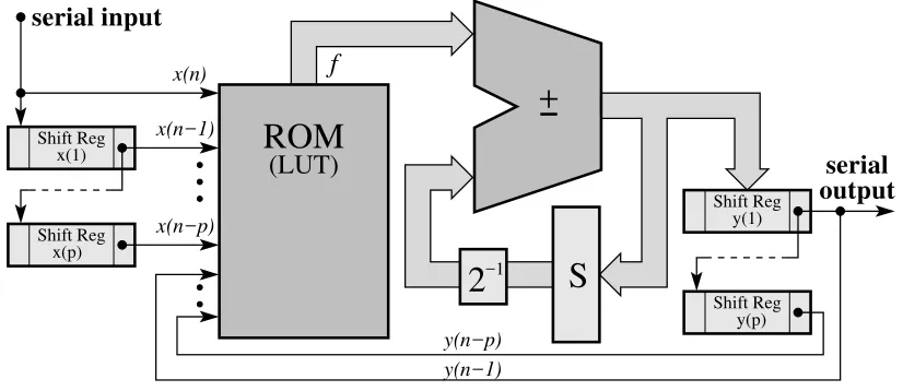
[image:3.595.56.537.114.230.2](3) Figure 1 shows the filter architecture (using Bit-Serial Arithmetic) to compute the equation 3, where the mappingf is presented as a Lookup Table (LUT) that includes all the possible linear com-binations of the filter coefficients, as was mentioned previously.
+
2
−1 serial outputS
f serial input x(n−1) x(n) x(n−p) y(n−1) y(n−p) (LUT)ROM
Shift Reg Shift Reg Shift Reg x(1) x(p) y(1) Shift Reg y(p)Figure 1: IIR-Digital Filter Architecture.
The architecture shown in Figure 1 has bit serial input and output. The ROM memory is addressed by the Least Significant Bits (LSB) of thex’s andy’s shift registers, and its output together with the
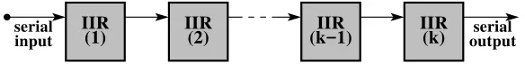
[image:3.595.93.506.455.634.2]We can construct high order filters by using the previously mentioned method, but the size required for the LUTs will grow exponentially with the number of filter coefficients. For this reason, a scheme is shown to construct high order IIR-filters making use of the properties of LTI systems such as association andcommutation. The associative property means that we may analyze a complicated LTI system by breaking it down into a number of simpler subsystems. The commutative property of LTI systems means that if subsystems are arranged in series, or cascade, then they can be rearranged in any order without affecting overall performance [7]. Therefore, interconnecting low order sub-filters appropriately we can make high order sub-filters. This technique permits us to use a set of smaller LUTs instead one huge LUT, which reduces considerably the space occupied in an FPGA. Figure 2 shows the interconnection scheme, where the input, the output and the internal connections (between the filters) are serials, and the(i)-filter output is connect to the(i+ 1)-filter input straight forward.
(1) (2) (k−1) (k)
IIR IIR IIR IIR
input
serial serial
[image:4.595.151.443.273.313.2]output
Figure 2: High Order IIR-Filter Interconnection Scheme.
For example, if we need to build a fifth-order IIR-filter we can use two second-order IIR-filters and one first-order IIR-filter. This allows us to use two 32-entry tables and one 8-entry table instead of one 2048-entry table.
3
FIR-DIGITAL FILTERS
In a FIR-Digital Filter the output depends only of present and previous input samples, which are multiplied by a set of coefficients and then added together to produce the output. The filter behaviour is determined by the filter coefficients. A general FIR-filter is characterized by the following equation:
yn=a
0xn+a1xn−1+· · ·+aqxn−p (4)
Wherepis the filter order, theap’s are the filter coefficients,xnis the input signal at the time step
n, andynis the output signal at the time stepn. The major disadvantage of these filters is that usually
a large number of coefficients are required to control adequately their frequency response. Practical FIR-Filters typically need between 10 and 150 coefficients. This make them slower in operation than most IIR-filter design.
Expanding the equation 4 forynin terms of the individual bits for the 2’C operandsx= (x(0).x(
−1)
x(−2)....x(−l))2andy= (y(0).y(−1)y(−2)....y(−l))2, like it was made for IIR-filter, we get:
yn=
−1
X
j=−l
2jf(xn
(j), xn(j−)1, . . . , x
n−p
(j) ) !
−f(xn
(0), xn(0)−1, . . . , x
n−p
(0) ) (5)
Figure 3 shows the filter architecture to compute the equation 5.
+
2
−1ROM
S
f
serial input
serial output
x(n−p) x(n−1) x(n)
(LUT)
Shift Reg. yShift Reg. x(1)
[image:5.595.93.506.97.274.2]Shift Reg. x(p)
Figure 3: FIR-Filter Architecture.
to this, afterl+ 1cycles, theadder-substractoroutput is only stored intoy(n)register.
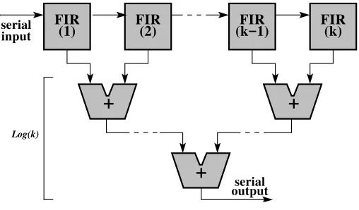
To construct high order FIR-filters we need to interconnect a cascade low FIR sub-filters; in that way the input pass through them serially and the sub-filters outputs are added (by serial adders) to produce the high order FIR-filter output. The interconnection scheme is shown in Figure 4.
FIR
(1) FIR(2) (k−1)FIR FIR(k)
+
+
+
Log(k)
serial input
serial output
Figure 4: High Order FIR-Filter Interconnection Scheme.
If we want to construct a high order FIR-filter making use of k sub-filters, its result will have
⌈log2(k)⌉additional bits due to the fact that the tree adder have depth⌈log2(k)⌉and each level may add one bit. Therefore, if the filter input havelbits the filter will produce one result eachl+⌈log2(k)⌉
clock cycles.
[image:5.595.168.422.416.565.2](a)
(b)
[image:6.595.128.468.95.587.2](c)
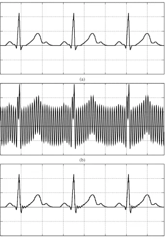
Figure 5: Removing mains-frequency interference from an electrocardiogram.
4
EXPERIMENTAL RESULTS
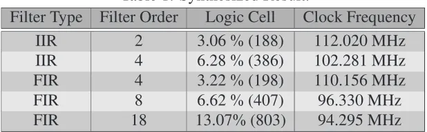
Table 1: Synthesized Result.
Filter Type Filter Order Logic Cell Clock Frequency IIR 2 3.06 % (188) 112.020 MHz IIR 4 6.28 % (386) 102.281 MHz FIR 4 3.22 % (198) 110.156 MHz FIR 8 6.62 % (407) 96.330 MHz FIR 18 13.07% (803) 94.295 MHz
To see the good behaviour of the architectures presented in the previous sections we will show the functioning of a digital filter. In particular, we will consider a digital filter for an electrocardiogram. In medicine, the electrical activity of the heart can be recorded using electrodes placed on the chest, a filter can be used to reduces the fluctuations due to electric activity in the resulting electrocardiogram (60 Hz in the USA, 50 Hz in Europe). In this case the needed digital filter is a band-stop IIR-filter, because we must reject the mains supply frequency (60 Hz or 50 Hz). This filter is characterized by the following equation:
yn=xn+ (−1.9021)xn−1+xn−2 + (1.8523)yn−1+ (−0.94833)yn−2 (6)
If the interference is at 60 Hz, the filter is effective at sampling frequency of 1200 samples per second (1.2 kHz); if it is at 50 Hz, the filter is effective at 1000 samples per second (1 kHz) [7]. The VHDL specification for this can be see in Appendix I. Figure 5 (a) shows a typical EKG waveform, corresponding to several heartbeat. In part (b) of the figure it is badly contaminated by sinusoidal in-terference of 60 Hz frequency. Figure 5 (c) shows the dramatic effect of this filter on the contaminated signal of part (b). The interference has been greatly reduced, without distorting the signal waveform.
Now, we will show the FPGA resources utilization of filters implemented with the techniques described in this paper. Table 1 presents these results. We can note that these techniques allow an important reduction in the logic cells utilization, also we can see that the size of filters grows lineally with the numbers of coefficients, degrading their performance slightly. We must have in mind that the overall performance of each implementation is: its clock frequency divide by the number of bits of its input signal (because this is processes serially). Therefore our implementations work at about 10 MHz, which is adequate for the most applications. These are important results, especially for FIR-filters, since they usually require many coefficients to control adequately their frequency response. In fact, using these techniques, we could synthesize a hundredth-order filter with a performance of 10 MHz approximately, it is not possible using traditional techniques with which we could synthesize sixtieth-order filters only.
5
CONCLUSION
REFERENCES
[1] Rawski, Tomaszewicz, Selvaraj and Luba. “Efficient Implementation of Digital Filters with Use of Advanced Synthesis Methods Targeted FPGA Architectures”.Digital System Design, 2005. Proceedings. 8Th Euromicro Conference on.30 Aug.- 3 Sept. 2005. Pages 460-466.
[2] Knut Arne Vinger and Jim Torrensen. “Implementing Evolution of FIR-Filters Efficiently in an FPGA”.Evolvable Hardware, 2003. Proceedings. NASA/DoD Conference on.July 9-11, 2003. Pages 26-29.
[3] Kalivas, Tsirikos, Bougas and Pekmestzi. “100% Operational Efficient Bit-Serial Programmable FIR Digital Filters”.EUSIPCO 2005- 13Th European Signal Processing Conference. Septem-ber 4-8, 2005. Antalya, Turkey.
[4] Chi-Jui Chou, Satish Mohanakrishnan and Joseph Evans. “FPGA Implementation of Digital Filters”. International Conference on Signal Processing Applications and Technology. Berlin, 1993. Pages 251-255.
[5] Sang-Hun Yoon, Jong-wha Chong and Chi-Ho Lin. “An Area Optimization Method for Digital Filter Design”.ETRI Journal, volume 26, Number 6.December 2004. Pages 545-553.
[6] behrooz Parhami. “Computer Arithmetic: Algorithms ans Hardware Designs”. New York: Ox-ford University Press, 2000.
APPENDIX I (VHDL CODE)
library IEEE;
use IEEE.std_logic_1164.all; use IEEE.numeric_std.all;
entity dig_filtro is port (
x : in unsigned(0 to 7);
clk : in std_logic;
rst : in std_logic;
y : out unsigned(0 to 7));
end;
architecture df of dig_filtro is
constant cBitsx : integer := 8;
constant cCoef : integer := 5; -- number of coeficient
constant cLogNumCoef : integer := 3; -- ciel of cCoef logaritm
constant cBitsM : integer := 8; -- number of coeficient bits
type TableCoef_type is array(0 to 2**cCoef-1) of
unsigned(0 to cBitsM+cLogNumCoef-1);
constant cTableCoef : TableCoef_type
:=(
signal x_n_reg : unsigned(0 to cBitsx-1);
signal x_n_input : unsigned(0 to cBitsx-1);
signal x_n_1_reg : unsigned(0 to cBitsx-1);
signal x_n_1_input : unsigned(0 to cBitsx-1);
signal x_n_2_reg : unsigned(0 to cBitsx-1);
signal x_n_2_input : unsigned(0 to cBitsx-1);
signal y_n_1_reg : unsigned(0 to cBitsx-1);
signal y_n_1_input : unsigned(0 to cBitsx-1);
signal y_n_2_reg : unsigned(0 to cBitsx-1);
signal y_n_2_input : unsigned(0 to cBitsx-1);
signal y_input : unsigned(0 to cBitsx-1);
signal y_reg : unsigned(0 to cbitsx-1);
signal counter_reg : unsigned(0 to cBitsx-1);
signal counter_input : unsigned(0 to cBitsx-1);
signal s_reg : unsigned(0 to cBitsM+cLogNumCoef-1);
signal s_input : unsigned(0 to cBitsM+cLogNumCoef-1);
signal f : unsigned(0 to cBitsM+cLogNumCoef-1);
signal opndo_1 : unsigned(0 to cBitsM+cLogNumCoef-1+2);
signal opndo_2 : unsigned(0 to cBitsM+cLogNumCoef-1+2);
signal add : unsigned(0 to cBitsM+cLogNumCoef-1+2);
signal address : unsigned(0 to 4);
begin -- df
counter_input <= counter_reg(counter_reg’high) &
counter_reg(0 to counter_reg’high-1);
x_n_input <= x when counter_reg(counter_reg’high)=’1’ else ’0’ & x_n_reg(0 to x_n_reg’high-1);
x_n_1_input <= x_n_reg(x_n_reg’high) & x_n_1_reg(0 to x_n_reg’high-1);
x_n_2_input <= x_n_1_reg(x_n_1_reg’high) & x_n_2_reg(0 to x_n_1_reg’high-1); y_n_1_input <= add(4 to 4+y_n_1_input’high) when
counter_reg(counter_reg’high) =’1’ else ’0’ & y_n_1_reg(0 to y_n_1_reg’high-1);
y_n_2_input <= y_n_1_reg(y_n_1_reg’high) & y_n_2_reg(0 to y_n_1_reg’high-1); y_input <= add(4 to 4+y_n_1_input’high) when
counter_reg(counter_reg’high)=’1’ else y_reg;
y <= y_reg;
opndo_1 <= ’0’ & s_reg(0) & s_reg(0 to cBitsM+cLogNumCoef-2) & ’1’; opndo_2 <= ’0’&(f xor (0 to (cBitsM+cLogNumCoef-1) =>
counter_reg(counter_reg’high)))& counter_reg(counter_reg’high);
add <= opndo_1 + opndo_2;
s_input <= (others => ’0’) when counter_reg(counter_reg’high) = ’1’ else add(1 to cBitsM+cLogNumCoef);
address <= (x_n_reg(x_n_reg’high), x_n_1_reg(x_n_1_reg’high), x_n_2_reg(x_n_2_reg’high), y_n_1_reg(y_n_1_reg’high), y_n_2_reg(y_n_2_reg’high));
with address select f <=
cTableCoef(3) when "00011", cTableCoef(4) when "00100", cTableCoef(5) when "00101", cTableCoef(6) when "00110", cTableCoef(7) when "00111", cTableCoef(8) when "01000", cTableCoef(9) when "01001", cTableCoef(10) when "01010", cTableCoef(11) when "01011", cTableCoef(12) when "01100", cTableCoef(13) when "01101", cTableCoef(14) when "01110", cTableCoef(15) when "01111", cTableCoef(16) when "10000", cTableCoef(17) when "10001", cTableCoef(18) when "10010", cTableCoef(19) when "10011", cTableCoef(20) when "10100", cTableCoef(21) when "10101", cTableCoef(22) when "10110", cTableCoef(23) when "10111", cTableCoef(24) when "11000", cTableCoef(25) when "11001", cTableCoef(26) when "11010", cTableCoef(27) when "11011", cTableCoef(28) when "11100", cTableCoef(29) when "11101", cTableCoef(30) when "11110", cTableCoef(31) when others;
write: process(clk,rst) begin
if rst=’1’ then
s_reg <= (others => ’0’); x_n_reg <= (others => ’0’); x_n_1_reg <= (others => ’0’); x_n_2_reg <= (others => ’0’); y_n_1_reg <= (others => ’0’); y_n_2_reg <= (others => ’0’);
y_reg <= (others => ’0’);
counter_reg <= (0 to counter_reg’high-1 => ’0’, counter_reg’high => ’1’);
elsif clk=’1’ and clk’event then counter_reg <= counter_input; s_reg <= s_input;
x_n_reg <= x_n_input; x_n_1_reg <= x_n_1_input; x_n_2_reg <= x_n_2_input; y_n_1_reg <= y_n_1_input; y_n_2_reg <= y_n_2_input; y_reg <= y_input;