LOUDNESS OF SOUNDS WITH TEMPORAL VARIABLE INTENSITY

LOUDNESS OF SOUNDS WITH TEMPORAL VARIABLE INTENSITY

PACS REFERENCE: 43.66

Meunier Sabine ; Marchioni Alain LMA-CNRS

31, chemin J. Aiguier 13402 Marseille cedex 20 France

33 491 16 41 75 33 491 77 55 65

[email protected]

ABSTRACT

In a pilot experiment on loudness of road-traffic noises, it has been shown that the loudness estimated by subjects could not be predicted by the value of N5 only (calculated using the model of Zwicker and Fastl, 1999). Nevertheless, it appeared that estimated loudness could be predicted by a combination of N5 and mean loudness averaged over time. Thus, we decided to run specific experiments on synthesized sounds, to get a precise control of these two parameters. Non-steady sounds were created with different profiles of amplitude variation in time (total duration of 6 s). These signals were a 1-kHz pure tone, the vowel « a » and a low-pass noise with a cut-off frequency of 4 kHz. For each category (pure tone, vowel and noise) two sets of signals were made: one with constant N5, the second with a constant mean loudness. Loudness was evaluated by 14 listeners using magnitude estimation. We looked for a model of loudness that would include both N5 and mean loudness. A forward regression between evaluated loudness, N5 and mean loudness shows that a model that does take into account mean loudness explains the major part of the variance of estimated loudness for the low-pass noise. For the pure tone, mean loudness and N5 explain a part of the variance, but the model must be improved. For the vowel, the result obtained cannot permit us to conclude.

INTRODUCTION

A lot of studies have shown that annoyance is highly correlated with loudness. This had been demonstrated for example by Berglund et al. (1976), among others, for community noise, and more recently by Canévet et al. (1999) in a study on environmental noises and by Altinsoy et al. (1999) in a study on noise produced by vacuum cleaners. Then, it is of a great interest to develop loudness models in order to have a tool to predict annoyance. Models of loudness have been developed by Zwicker and his colleagues (Zwicker and Scharf, 1964; Zwicker et al., 1984) and more recently by Moore and his colleagues (Moore and Glasberg, 1996; Moore et al., 1997). For stationary sounds, the estimated loudness is well predicted by the models (Fastl, 1985; Meunier, 2000). But, most of environmental sounds are not stationary.

noises, the percentile loudness N10 does not describe well the estimated loudness. Therefore, experiments with synthetic sounds have been run to investigate the relationship between overall loudness judgment and the temporal pattern of loudness. The advantage of synthetic sounds is that the physical parameters of the signals can be totally controlled. Then, sounds with different temporal shapes were built, allowing to set the N5 constant and to investigate the influence of other parameters like the mean loudness.

PRELIMINARY EXPERIMENT

In a study on annoyance of road-traffic and train noises (Meunier et al., 2000a; Meunier et al., 2000b), different perceptual parameters have been measured for a group of sounds with the same loudness. The aim of the experiment was to find out the relationship between annoyance and acoustical and/or psychoacoustical parameters, discarding the influence of loudness. The loudness of the sounds was equalized on the basis of N10. Afterwards, different perceptual parameters were evaluated by the subjects using seven-step continuous scales. Among them, a scale named "loud" was used to measure loudness. The two end points of the scale were labeled "not very" and "very". The experiment has been run on road-traffic and train noises. Road-traffic noises were very instationary compared with train noises, which were quasi-stationary.

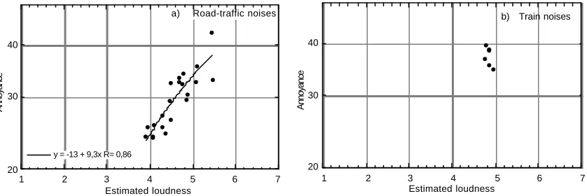
The method of magnitude estimation developed by Stevens (1975) was used to measure annoyance. In figure 1a and b, annoyance is plotted versus estimated loudness for the road-traffic noises and the train noises respectively.

20 30 40

1 2 3 4 5 6 7

y = -13 + 9,3x R= 0,86

Annoyance

Estimated loudness

a) Road-traffic noises

20 30 40

1 2 3 4 5 6 7

Annoyance

Estimated loudness

b) Train noises

Figure 1: Annoyance as a function of estimated loudness: a) For road-traffic noises

b) For train noises

One can observe on figure 1b that, for the train noises, estimated loudness is, as expected, constant within the corpus of sounds. On the other hand, for road-traffic noises, the estimated loudness varies within the corpus of sounds (figure 1a). Furthermore, it should be noted that, even if loudness variation is low, annoyance is correlated with loudness with a correlation coefficient of 0.86.

The result obtained for the train noises is not surprising because these noises are quasi-stationary and, in this case, N10 is close to what would have been the loudness calculated using a model for stationary signals.

EXPERIMENT

The aim of this experiment is to investigate how loudness is evaluated by subjects for different sorts of time-varying signals.

Stimuli and method

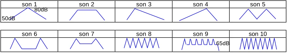
Three sounds with different temporal fine structures have been chosen: a 1-kHz pure tone, the vowel "a" and a low-pass noise with a cut-off frequency of 4 kHz. For each sound, twelve temporal envelopes have been defined (table 1). The level of the envelopes varied from 50 dB to 80 dB. All sounds had duration of 6 s.

son 1 son 2 son 3 son 4 son 5

son 6 son 7 son 8 son 9 son 10

Table 1: Temporal envelopes of the sounds

Two sets of signals were made: in the first one, the percentile loudness N5 was kept constant and in the second one, the mean loudness was kept constant. The levels of the original sounds (table 1) were slightly modified to equalize on the one hand N5 and on the other hand the mean loudness. Thus, 20 sounds have been synthesized for the 1-kHz pure-tone (temporal fine structure): 10 sounds (with envelopes shown in table 1) with a N5 of 78 phons (±1.5 phon) and 10 sounds (with the same envelopes) with a mean loudness of 66 phons (±1 phon). In the same way, 20 sounds have been synthesized with the vowel and the low-pass noise. For the vowel, N5 was set at 87 phons (±1 phon) and mean loudness at 73 phons (±0.3 phon). For low-pass noise, N5 was set at 93.5 phons (±1 phon) and mean loudness at 80 phons (±0.5 phon).

The mean loudness level and the percentile loudness N5 level were calculated using a matlab program computed from the model given by Zwicker and Fastl (Zwicker, 1977; Zwicker, 1984; Zwicker and Fastl, 1983).

The experiment was run in an anechoic chamber. The sounds were played via a loudspeaker (Genelec 1031A). The loudness was estimated using magnitude estimation without reference (Steven, 1975). In a run, the subject had to judge the loudness of one category of signal (pure tone, vowel or low-pass noise). Each run was separated by a 5-min pause. Within each run, the sounds with a constant N5 and those with a constant mean loudness were mixed and presented in random order. The order of presentation of the three run was different from a subject to another. Fourteen persons volunteered to be subject for this study.

Results

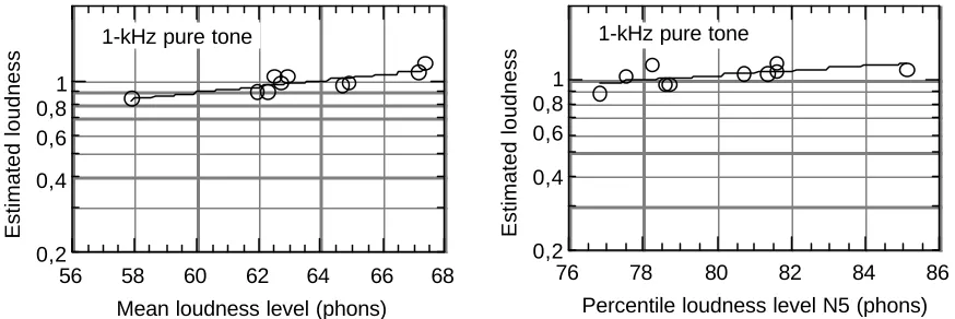
The data were normalized by dividing, for each run, each individual listener's estimation by the geometric mean of all of that individual's estimation. The geometric mean of the group is plotted versus calculated loudness level in figures 1 to 3. The graphs on the left of the figures shows estimated loudness as a function of calculated mean loudness level, N5 being constant. The graphs on the right of the figures shows estimated loudness as a function of calculated N5, mean loudness being constant.

On can observe that the slope of the function between, on the one hand, estimated loudness and N5 and, on the other hand, estimated loudness and mean loudness level depends on the spectra of the sound (see the curving fits in figure 1 to 3).

50dB

80dB

stepwise forward regression was run for the three sorts of sounds. The estimated loudness was the independent variable and N5 and mean loudness level the dependent variables. The regression was calculated on the logarithms of the estimated loudness, to get linear series of data. Indeed, with magnitude estimation, the series of data is geometric.

0,2 0,4 0,6 0,8 1

56 58 60 62 64 66 68

Estimated loudness

Mean loudness level (phons) 1-kHz pure tone

0,2 0,4 0,6 0,8 1

76 78 80 82 84 86

Estimated loudness

Percentile loudness level N5 (phons) 1-kHz pure tone

Figure 1: Estimated loudness as the function of calculated mean loudness level (left) and calculated N5 loudness level (right) for a 1-kHz pure-tone.

0,2 0,4 0,6 0,8 1

66 68 70 72 74 76 78

Estimated loudness

Mean loudness level (phons) Vowel

0,2 0,4 0,6 0,8 1

84 86 88 90 92 94

Estimated loudness

Percentile loudness level N5 (phons) Vowel

Figure 2: same as figure 1 for the vowel "a".

0,2 0,4 0,6 0,8 1

74 76 78 80 82 84

Estimated loudness

Mean loudness level (phons) Low-pass noise

0,2 0,4 0,6 0,8 1

90 92 94 96 98 100

Estimated loudness

Percentile loudness level N5 (phons) Low-pass noise

Figure 3: same as figure 1 for the low-pass noise.

Variable R R2 R2mod p Mean loudness level 0.82 0.67 0.67 0.000011

N5 0.84 0.71 0.04 0.13

Table 2: correlation coefficients from a stepwise forward regression. In the second line (mean loudness level), the correlation between logarithm of estimated loudness and mean loudness level is

given. In the third line, the correlation when N5 is added to the model is given. R2mod is the increase of R2.

For the vowel, the stepwise forward regression showed that 22% of the variance of the estimated loudness could be explained using a model with the mean loudness level. The percentile level N5 has no influence on the variance of the estimated loudness and thus it was not added to the model. But, in figure 2 (left graph), on can observe an outlier point on the left part of the graph (abscissa ~ 67 phons). This outlier point was removed of the analysis. The stepwise forward regression was run without this point and no correlation have been found between variables.

In figure 3, on can observe an outlier point on the left part of the graph, it has been removed of the analysis. Table 3 shows the result for the low-pass noise. The stepwise forward regression shows that 99% of the variance of the estimated loudness can be explained by a linear relationship to mean loudness level (table 3, R2 = 0.99). It was found that the percentile loudness level N5 has no influence on the variance of the estimated loudness and thus it was not added to the model.

Variable R R2 p

Mean loudness level 0.996 0.99 <0.0001

Table 3: same as table 2 for the low-pass noise.

CONCLUSION

In this paper we have shown, in the case of a 1-kHz pure tone, a vowel and a low-pass noise, how the estimated loudness can be related to mean loudness level and percentile loudness N5 (both calculated using loudness' model). The idea of the study was to keep constant the mean loudness level of the signal and to investigate how loudness varies with the percentile loudness level N5. Then the reverse was done, that is, N5 was kept constant and we have investigated how loudness varies with mean loudness level. It is observed that, for the pure tone and the noise, mean loudness level predict most part of the overall estimated loudness of time-varying sounds and that the addition of N5 does not increase significantly the percentage of variance explained. For the vowel, no significant results have been found, and hence it is difficult to conclude now.

The results are surprising. It seems that N5 has no influence on estimated loudness. This could be due to the sample of signals used, their envelopes and their levels. Especially for the vowel and the low-pass noise, where, if the outlier points are discarded, the range of the level is only of 4 phons.

This study shows that N5 is not sufficient to evaluate the loudness of time-varying sounds. Mean loudness should be taken into account. But at this point of the research, more experiment should be done to clarify the results.

Altinsoy E., Kanca G. and Belek H. T. (1999). "A comparative study on the sounds quality of wet-and-dry type vacuum cleaners", Proceedings of the 6th International Symposium on Sound and Vibration, Copenhagen, Denmark.

Berglund B., Berglund U. and Lindvall T. (1976). "Scaling loudness, noisiness and annoyance of community noises", J. Acoust. Soc. Am., 60, 1119-1125.

Canévet G., Meunier S. Marchioni A., Regal X., Carles J. L. and López Barrio I. (1999). "Nuevos estudios de validaçion subjetiva de los indices de calidad sonora", Proceedings of the Meeting of the acoustical Society of Spain, Ávila 20-22 october, Cdrom, 1-8.

Fastl H. (1985). "Loudness and annoyance of sounds : subjective evaluation and data from ISO 532B", Inter noise 85, 1403-1406.

Meunier S. (2000). "Subjective evaluation of loudness models using synthesized and environmental sounds", Inter noise 2000, vol.4, 2205-2209.

Meunier S., Boussard P., Marchioni A. Rabau G., Regal X. et Santon F (2000a). "Simulation acoustique et évaluation psychoacoustique de bruits de circulation routière", Proceedings of the 5th French Congress on Acoustics, Lausanne, Suisse.

Meunier S., Santon F., Boussard P., Marchioni A. Rabau G. et Regal X. (2000b). "Etude perceptive de bruits de circulation routière et ferroviaire", Research Report, PREDIT 98.

Moore B. C. J. and Glasberg B. R. (1996). "A revision of Zwicker's loudness model", ACUSTICA-Acta acustica, 82, 335-345.

Moore B. C. J., Glasberg B. R. and Baer T. (1997). "A model for the prediction of thresholds, loudness and partial loudness", J. Audio. Eng. Soc., 45, 224-240.

Stevens S. S. (1975). Psychophysics, New-York, John Wiley.

Zwicker E. (1977). "Procedure for calculating loudness of temporally variable sounds", J. Acoust. Soc. Am., 62, 675-681.

Zwicker E. (1984). "Dependence of post-masking on masker duration and its relation to temporal effects in loudness", J. Acoust. Soc. Am., 75, 219-223.

Zwicker E. and Fastl H. (1983). "A portable loudness-meter based on ISO 532B", Proceedings of the 11th International Congress on Acoustics, Paris.

Zwicker E. and Fastl H. (1990). Psychoacoustics : facts and models, Springer.

Zwicker E. and Fastl H. (1999). Psychoacoustics : facts and models, Springer, 2d Updated Edition.

Zwicker E. and Scharf B. (1965). "A model of loudness summation", Psychological Review, 72, 3-26