Universidad Nacional de La Plata
Novenas Jornadas de Economía
Monetaria e Internacional
La Plata, 6 y 7 de mayo de 2004
Estimating Household Responses to Price Reforms: Trade,
Agricultural Income and Labor Supply in Mexico
Estimating Household Responses to Price Reforms.
Trade, Agricultural Income and Labor Supply in
Mexico
∗
Guido G. Porto
†Development Research Group
The World Bank
May 2004
Abstract
Economic reforms involving the agricultural sector, such as those being proposed in the WTO Doha Round negotiations, will affect household behavior in developing countries. This paper proposes an empirical methodology to assess the impacts of agricultural price reforms on household outcomes like consumption patterns, sources of income, labor supply, health outcomes, and educational decisions. The method uses an empirical model of demand to extract price information from unit values, and uses this information to estimate the response of households to price changes and price reforms. By correcting unit values for quality effects, the method overcomes the endogeneity and measurement error problems of using unit values as regressors. The methodology is applied to study the responses of household agricultural labor income and labor supply in rural Mexico. I find that higher prices of corn and fruits and vegetables, key goods produced in rural Mexico, significantly increase the agricultural wage income of rural Mexican households. Instead, corn prices do not seem to affect the labor market decision of young adults. It is shown that using unit values instead of prices may lead to inconsistent results, and that the corrections suggested in this paper may be empirically important.
∗Very preliminary note. Comments are welcome. The outstanding research assistance of Jorge Balat is
greatly appreciated. I thank I. Brambilla, A. Deaton, P. Goldberg and G. Grossman for useful comments on an earlier version of this paper. I assume full responsibility for all the errors and omissions. Comments and suggestions are very much welcome. The views expressed here are my own and are not necessarily endorsed by the World Bank Group.
†Correspondence: Guido Porto, MailStop MC3-303, The World Bank, 1818 H Street, Washington DC
1
Introduction
This paper proposes an empirical method to evaluate price reforms. The method provides an
alternative that can be used when natural or quasi experiments (Meyer, 1995) or matching
methods (Rosenbaum and Rubin, 1983) are not feasible alternatives. Trade reforms are an
example: trade liberalization is often accompanied by other simultaneous reforms and it is
often difficult to identify the treatment and control groups. In many instances, in addition, there is an interest, or a need, to explore the effects of a policy that has not yet taken place.
The method proposed here accommodates these cases.
Most policy reforms can be linked to price changes. In consequence, one way to evaluate
the impacts of economic policies is by estimating the responses of some household behavior
to prices and then to link prices with the reforms. Although conceptually attractive, there
are several empirical difficulties with this two-step approach. One in the need to estimate
structural models so that household responses can be linked to prices through a structural
parameter that can be used to simulate policy outcomes.1 More importantly, there is a need
of survey data with sufficient price variation at the household level. This is rarely the case.
The current practice is to proceed with the following alternatives. One is to combine
household surveys with official price information. Often times, there is time and regional
variation in prices. Examples include Deaton (1997), Porto (2003), Ravallion (1990), and
Wolak (1996). In some surveys there are community price questionnaires that provide more
variation in prices. Edmonds and Pavcnik papers on Viet Nam are outstanding examples
(Edmonds and Pavcnik, 2003, 2004). Another option is to use unit values as measures of
prices. In many surveys, households are asked to report expenditures and quantities bought
of several goods. The ratio of these quantities, the unit values, provide useful information
on prices that can be used to assess price reforms (Balat and Porto, 2004).
The use of unit values in household models has advantages and disadvantages. The
main advantage is that, at least for food items, many households provide information on
expenditures and quantities, so that unit values are available at the household level. This
introduces a lot of cross-sectional variability. However, it has long been argued that unit
values are not the same as prices. Deaton (1987), for instance, showed that consumers jointly
choose quantity and quality so that unit values combines measures of price and quality. Thus,
the use of unit values instead of prices may contaminate the regression model and lead to
misleading results in the evaluation of policies.
In a series of seminal papers, Deaton (1987, 1988 and 1990) proposed a methodology
to account for the difference between prices and unit values. With the aim of examining
tax reforms in developing countries, he applied these methods to estimate demand systems
and to recover own- and cross-price elasticities. Deaton’s main insight is to model consumer
choices of quantity and quality simultaneously in order to extract the right price signals from
the data on unit values.
In this paper, I propose a joint estimator of demand price-elasticities and a household
outcome price-elasticity (or a household behavior price-elasticity). These parameters could
be used to assess a number of policies, including trade liberalization, agricultural reforms, and
tax reforms. Suitable household outcomes may include the wage earned by the household head or the agricultural income of different households. Suitable behaviors may include the labor supply of different individuals (including children and women), health status, or
education.
The procedure extends the empirical model of demand developed by Deaton by
endogenizing how prices determine some household outcome (wage agricultural income) or
some household behavior (labor choice, occupational choice). The model of demand allows
me to extract price information from unit values, expenditures, and quality choices, as in
Deaton’s work. My extension shows how to use this price information to estimate the
response of household outcomes.
In this paper, I develop the econometric model and I provide the formulas for the general
case. After developing the formulas, I put them to work by studying one household outcome
and one household behavior in rural Mexico. The household outcome studied here is the
response of agricultural wage income to agricultural prices such as corn, wheat, dairy, oils
market participation of young adults to those agricultural prices. In order to assess the
proposed methodology, I estimate the models of household outcome and household behavior
under the assumption that unit values can be correctly used as measures of prices.
I find that higher prices of corn and fruits and vegetables, key goods produced in rural
Mexico, significantly increase the agricultural wage income of rural Mexican households.
Further, the probability that young adults participate in the labor market depends positively,
but not significantly, on the price of corn. It is shown that using unit values instead of prices
may lead to inconsistent results, and that the corrections suggested in this paper may be
empirically important. Alternative models with partially purged unit values (instead of fully
quality corrected unit values) are explored as well. These alternatives, of lower accuracy but
easier implementation, seem to work well in practice.
The paper is organized as follows. Section 2 provides a more general motivation of
the paper and gives an overview of the methodology. I develop a simplified version of the
model with only one good, as in Deaton (1997), to clarify the intuition and the mechanism
through which Deaton’s method can be extended to identify the effects of price changes
on household outcomes. Section 3 develops the full model, with possibly many agricultural
prices affecting outcomes. Section 4 applies the method to the Mexican data and reports
the empirical results. Section 5 concludes.
2
Motivation
Let’s assume that the interest lies in the estimation of the response of agricultural wage
income in rural Mexico to the WTO agricultural trade negotiations. The case of Mexico
is, in principle, a good case study because of the importance of the agricultural sector and
because of the proximity of the country to the United States. More concretely, suppose that
the United States and the European Union eliminate production and export subsidies on
corn and that, as a result, its international price increases. Corn is a key agricultural good
in Mexico and I expect changes in its price to significantly affect outcomes and behavior
in agricultural activities, such as farm labor and agricultural services. In consequence, the wage agricultural income of rural households may be affected.
A good staring point in the estimation strategy would be to use the Mexican household
surveys. These are the Household Income and Expenditure National Surveys, ENIGH
(Encuesta Nacional de Ingresos y Gastos de los Hogares).2 These surveys collect data on expenditure and quantities bought of different agricultural goods, including corn; data on
sources of household income is collected, too. Let vc be the average unit value of corn
reported by households residing in cluster c. The simplest model would regress agricultural
wage income, ahc, on average unit values and additional controls m,
(1) lnahc=α+γmhc+λln(vgc) +uhc.
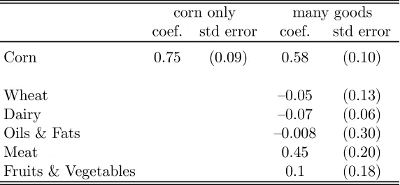
In column 1 of Table 1, I report the results of a regression of the agricultural wage income of
rural households on a number of household controls (such as household size, demographics,
education of the head, and year dummies) and the log of the average unit value spent on
corn. Ifind thatahcis positively and significantly associated with corn prices. The elasticity
is 0.75, with a t statistic of 7.6.3 This is an intuitive result. Since corn is one of the main
goods produced in rural Mexico, higher corn prices induce households, farms and firms to
devote more resources to corn production and thus labor demand in agricultural activities
increases. In the end, the agricultural wage income of rural households will increase.4
In column 2 of Table 1, I add the prices of other agricultural goods, such as wheat, dairy,
oils & fats, meat and fruits & vegetables. It is still found that the price of corn positively
affects agricultural income, with an elasticity of 0.58 and atstatistic of 5.65. Apart from the price of meat, which appears to affect wage agricultural income positively too, the remaining
prices are statistically insignificant.
There are three concerns with a regression model such as (1): endogeneity of unit
2See Apendix 1 for a description of the data.
3Notice that the standard errors are corrected for clustering since all households in a given cluster face the same averages for the unit values.
4Notice that I am estimating equilibrium responses in wage agricultural income. For instace, it may be the case that labor supply increases as a result of higher corn prices, probably causing wages to decline. My
Table 1
Simple Models of Agricultural Wage Income Using Average Unit Values
corn only many goods coef. std error coef. std error Corn 0.75 (0.09) 0.58 (0.10)
Wheat —0.05 (0.13)
Dairy —0.07 (0.06)
Oils & Fats —0.008 (0.30)
Meat 0.45 (0.20)
Fruits & Vegetables 0.1 (0.18)
Note: estimates from the simple model that uses OLS and average cluster unit values as regressors. The first model includes the price of corn as the only price regressor. The second model includes other agricultural prices. The standard errors (which are cluster corrected) are reported in parenthesis. The regressions include a number of additional controls, such as demographics, education, age, gender and year dummies.
values, bias due to proxy variables, and measurement error. Endogeneity may arise because
households choose quantity and quality together; unit values are not a perfect measure of
prices. Even when unit values are a good proxy for prices, the model may estimate the
vector γ consistently, but λ inconsistently. Measurement error arises if there are inaccurate
responses, mainly on quantities consumed. In all these cases, OLS estimation of (1) will
lead to inconsistent estimates of the wage agricultural income price-elasticity. The results
shown in Table 1 suggest that these problems may indeed be present. Attenuation bias due
to measurement error, for instance, may be critical: all the unit value regressors, except for
corn and meat, are not statistically significant. Some of these problems could be solved by
using an instrumental variable estimator instead of OLS. If finding suitable instruments is
difficult, as it probably is since household variation is generally desirable in the instruments,
the estimation of (1) will not produce consistent results.
The method proposed in this paper combines a model such as (1), with true unobservable
prices instead of average unit values as regressors, with the model of demand and quality
shading developed by Deaton (1988). In order to introduce the method, I begin by setting up
rather, my aim is to provide an intuition for the more difficult formulas derived in Section 3.
The demand for the good is modeled with an equation characterizing budget shares (the
implicit assumption is that there are other goods that complete the system). Deaton and
Muellbauer (1980) show that a suitable model for the budget share shc spent by household
h in cluster c (a village, for example) is
(2) shc =α0+β0lnxhc+γ0zhc+θlnπc+fc+u0hc,
wherexhcis total expenditure,zhcare household demographic characteristics, such as number
of members and demographic composition. πc is a price level that is assumed to be the same
for all households in cluster c; this price is unobservable. fc is a fixed effect at the cluster
level andu0
hc is a standard error term, with zero mean (for a large number of households in
each cluster) and variance σ00.
The endogeneity of unit values may be solved by modeling unit values explicitly. Unit
values are not the same as prices; rather, they are function of the priceπc. I assume that
(3) lnvhc =α1+β1lnxhc+γ1zhc+ψlnπc+u1hc.
Here, unit valuesvhcare affected by household expenditurexhc. As explained by Deaton, the
parameterβ1 is called the “quality elasticity” or the “expenditure elasticity of quality”. This
parameter β1 would be zero if there were no quality shading. Demographics zhcdetermine
unit values, too. The error termu1
hc has mean zero (for a large number ofhin clusterc) and
variance σ11. There is nofixed effect in this equation, for identification purposes.
Equations (2) and (3) are modeled exactly as in Deaton (1997). My extension introduces
into this model a way to handle the endogenous determination of household wage agricultural
income,ahc. I redefine (1) as
(4) lnahc=α2+γ2mhc+λlnπc+u2hc,
different from the determinants of the budget shares and unit value), such as education,
age, or marital status of the income earner; u2
hc is an error term. There is no fixed effect
in this equation either. The coefficient λ measures the price elasticity, or the proportional
change in agricultural income brought about by the changes in product prices.
The model is estimated in two stages. If prices πc were observed, it would be
straightforward to estimate the model in (2), (3) and (4). This is a system of equations that
can be handled easily with well-known econometric techniques. Prices πc are not observed
though. The identification assumption is that every household in cluster c faces the same
prices. This implies that unobserved prices can be controlled for with cluster dummies (which
will absorb anyfixed effects as well). In the first stage, then, I recoverβ0,γ0, β1, γ1 andγ2
by estimating the model by OLS, after demeaning all variables (shc,lnvhc,lnahc,lnxhc, zhc,
andmhc) from cluster means.
With estimates β0e , eγ0, β1e ,eγ1 and eγ2, I construct three variables
(5) yehc0 =shc−β0ˆ lnxhc−ˆγ0zhc,
(6) yehc1 = lnvhc−β1ˆ lnxhc−eγ1zhc,
(7) yehc2 = lnahc−eγ2mhc.
Averaging (5), (6) and (7) at the cluster level, I argue that
(8) yec0 p
−→α0+θlnπc+fc+u0c,
(9) yec1 −→p α1+ψlnπc+u1c,
(10) yec2 −→p α2+λlnπc+u2c,
whereu0
c,u1c, andu2c are average error terms in clusterc (these averages would be zero for a
Notice that
(11) covf ye0c,ye1c
− eσ 01
nc
=θeψevar(lnπc),
(12) covf ye0c,ye2c
− eσ 02
nc
=θeeλvar(lnπc),
where nc is the number of observations (households) in cluster c, σe01 is the estimated
covariance between the residual in the equation for budget shares and the equation for unit
values, and eσ02 is the estimated covariance between the residual in the equation for budget
shares and the equation for wage agricultural income. By the same token, notice that
(13) gvarye1c
− 1
nce
σ11 =ψe2var(lnπc),
(14) gvarye2c
− 1
nce
σ22 =eλ2var(lnπc),
where eσ11 and eσ22 are estimates of the variances of the residuals in the equations for unit
values and wage agricultural income. By combining (11), (12), (13) and (14), I can identify
the ratios φ1e =θe/ψeandφ2e =θe/eλ.
To recover the elasticities, I combine these estimates with a quality shading model. I
borrow Deaton’s group-separable preference model of demand. Let p be the price elasticity
of quantity with respect to priceπ and let x be the total expenditure elasticity of the group.
Deaton (1988) shows that
(15) ψ = 1 +β1 p
x
.
While Deaton was interested in the elasticity of demand p and the expenditure elasticity x,
here I am after an estimate of λ, obtaining p and x as intermediate steps.
I assume that total household expenditure comprises agricultural wage income,ahc, other
labor income whc, and capital income khc, so that
Adapting Deaton’s formulation, it is possible to show that
(17) ψ = θ
s +bwλ−εp,
where sis the average budget share andbw is the share of wage agricultural income in total
income. Finally, Deaton (1997) shows that
(18) β1 = β0
s + 1−εx.
Using (15), (17) and (18), it follows that
(19) ψ = 1 +β1
θ
s +bwλ−ψ
β0
s + 1−β1
.
This equation can be combined with the estimates ofφ1e andφ2e to solve forθe, ψeandeλ, the
agricultural income price elasticity.
To exemplify how the simplified model works, I estimate it for the case of corn. Ifind an
elasticity of 0.95, with a tstatistic of 6.79. These numbers are in line with those reported in
Table 1. A generalization to the case of many goods follows.
3
The Full Model
In this section, I provide the formulas needed to implement the full model, with
many agricultural goods, cross-price elasticities and several agricultural wage income
price-elasticities. To extend the simplified model, I begin by rewriting the general formulas
for budget shares, unit values and agricultural wage income. With G goods, the budget
share spent on goodg by household h(in cluster c) is
(20) sghc =α g
0+β
g
0 lnxhc+γ0gzhc+
[
k G
θgklnπck+f g c +u
g0
where lnπk
c is the (log) price of good k in cluster c. As before, fcg is a fixed effect at the
cluster level and ughc0 is the error term, with mean zero and variance σ00g . This model of
demand is similar to the AIDS model of Deaton and Muellbauer (1980b).
The unit value equation for good g is
(21) lnvhcg =αg1+β1glnxhc+γ1gzhc+
[
k G
ψgklnπck+u g1
hc.
Here, the “quality elasticity” for good g is β1g. The error term ughc1 has also zero mean and
variance σg11. This is just the generalization to many goods of equation (3).
There areG equations (20) and (21); instead, there is only one agricultural wage income
equation
(22) lnahc=α2+γ2mhc+
[
k G
λklnπkc +u2hc,
where u2
hc is an error term. As argued above, changes in prices, particularly of agricultural
goods, will cause some agricultural activities to expand and some others to contract. This,
in turn, will lead to changes in agricultural labor demand and supply and, in the end, to
changes in the agricultural wage income of rural households. Equation (22) captures these
effects.
In the first stage, I demean budget shares, log unit values and log agricultural income to
eliminate prices and clusterfixed effects. In principle, there is no problem with the consistent
estimation of these parameters if the regressors are exogenous, as in Deaton (1990). Here,
however, I am introducing an agricultural wage income equation and agricultural income
may be correlated with total expenditure. This means that the model is not identified if
there is correlation between the errors of the share or unit value equations with the error of
the wage agricultural income equation.
If I assume that this correlation is absent, then the model is triangular and I can estimate
it consistently using OLS equation by equation. This assumption is not necessary. It
parameters of the demeaned model using instruments in the share and unit value equations.
In particular, since the set of explanatory variables in mhc is different from the set of
explanatory variables in zhc, I use the variables that are in m but not in z as instruments.
These exclusion restrictions allow me to fully identify the parameters of thefirst stage. The
parameters of the agricultural wage income equation are identified providedmis exogenous,
which I assume.
For each good g, I build the following variables
(23) yecg0 =
1 nc
[
h
sghc−βeg0lnxhc−eγ g
0zhc
,
(24) yecg1 =
1 nc
[
h
lnvhcg −βeg1lnxhc−eγ1gzhc
,
(25) yec2 =
1 nc
[
h
(lnwhc−eγ2zhc).
The population counterparts are
(26) yecg0 −→p αg0 +[
k G
θgklnπck+f g c +u
0
cg,
(27) yecg1 p
−→αg1 +
[
k G
ψgklnπck+u1cg,
(28) ye2
c p
−→α2+
[
k G
λklnπck+u2c,
where u0
cg, u1cg, and u2c are average error terms in clusterc.
To solve for the parameters of interest (i.e. the price elasticities), I need to extend the
quality model to many goods. This is done in Deaton (1988) and Deaton (1990), who shows
that
(29) ψgk =δgk+β1g
gk p
g x
,
of good k and g
x is the expenditure elasticity. The generalization of equation (19) is
(30) ψgk =
θgk
sg
+bwλk− gkp .
Finally, I have that, for each good g
(31) β1g = β
g
0 sa
+ 1− g x.
Combining (29), (30) and (31), it follows that
ψgk =δgk+
β1g β0g +sg(1−β
g
1)
[θgk+sgbwλk−sgψgk].
Defining a vector ξ with elementβ1g/(β0g+sg(1−β g
1))for goodg, and a vector sof average
budget shares, I can write
(32) Ψ=I+D(ξ)Θ+bwD(ξ)D(s)Λ−D(ξ)D(s)Ψ,
whereD(ξ)andD(s)are matrices with the elements of vectorsξ andson the diagonal (and
zero off-diagonal elements). The matrix Λ is defined as
(33) Λ=1G⊗λ,
where 1G is a G×1 vector of ones and λ is a G×1 vector of agricultural income price
elasticities λg.
To solve for λ, I need to manipulate the model and introduce some new notation, as
follows. Let πc be a 1× G vector of the logarithm of (unobserved) prices in cluster c.
Stacking the vectors πc for all clusters, I get a C ×G matrix π. I stack observations on
average unit values for good g, (24), into a C×1 vector ey1g = 1Cαg1 +πψg+u1g, where 1C
follows that
(34) cov(ey1g,ye1k) =ψgΠψk+E[u1gu1k],
where Π is the variance-covariance matrix of the vector of good prices (across clusters).
Next, I construct a G×Gmatrix V1 with element gk given by (34)
(35) V1 =ΨΠΨ +Ω11,
where Ω11 is the matrix withgk element E[u1gu1k].
Following the same procedure, I generate the vectorye0g by stacking the estimated average
budget shares spent on good g by clusters. This vector isye0
g = 1Cα0g+πθg +fc+u0g,where
θg is the gthrow of matrix Θ, and u0g is a vector of residuals. It follows that
(36) cov(ey1g,ye0k) =ψgΠθk+E[u1gu0k].
Next, I build a G×G matrix V10 with elementgk given by (36)
(37) V10 =ΨΠΘ +Ω10,
where Ω10 is the matrix withgk element E[u1gu0k].
So far, I have shown how estimation of the model of demand delivers algebraic expressions
involving the unknown matricesΘandΨ; these are equations (35) and (37). These equations
can be combined to express one of these matrices as a function of the other. For instance,
by defining a matrixB = [V1−Ω11]−1[V10−Ω10], it follows that
(38) BΨ=Θ.
The next step is to complete the system by developing similar formulas involving the vector
λ of wage agricultural income price elasticities. One option is to combine the agricultural
clustercas a stacked vectorye2 =1Cα2+πλ+u2, Ifind that the covariance between ey2 and
e y1g is
(39) cov(ey2,ye1g) = λΠψg+E[u2u1g].
This allows me to build a G×1 vector v21 with elementg given by (39)
(40) v21=ΨΠλ+ω21,
where ω21 is a vector with g element E[u2u1
g]. Next, I define a matrix B1 = [v21−ω21] [V1 −Ω11]−1, so that
(41) B1 =λΨ−1.
These are all the steps needed to close the model. The mechanics of the solution involves
using (32), (38) and (41) to solve for the matrices Θ and Ψ, and the vector λ. Replacing
(38) and (33) in (32), I get
e
Ψ= [I−D(ξ)B −bwD(ξ)D(s)1G⊗B1+D(ξ)D(s)]−1.
This matrix is a function of the data, and can be estimated after B and B1 have been
computed from the data. Plugging this into (38) and (41), I get
e
Θ=BΨe,
e
λ =B1Ψe.
This vectoreλ is the vector of agricultural income price-elasticities that are needed to jointly
assess, for instance, the effects of trade reforms on income and expenditure. This is discussed
3.1
A Special Case
The model described so far is quite general. By allowing for the estimation of a wage
agricultural equation, a number of complications arose. Changes in prices bring about
changes in demands but also changes in wages. This means that the total expenditure of the
household may change when prices change. In consequence, the typical model of demand with
exogenous expenditure (Deaton and Muellbauer, 1980a) had to be modified to account for the additional effects of prices on quantities via changes in expenditure. Another important
complication was that the agricultural income equation introduced an endogeneity problem
in the estimation of the first stage. In some potential applications, these complications are
not present, and the estimation of the model can be simplified. A special case that is not
subject to these problems is when the interest lies, for example, in the estimation of the
effects of price reforms on behavior, such as health, nutrition, education, and labor market
participation.5
The extension is simple. The budget share and unit values equations remain intact. I
replace the agricultural income equation with an “outcome” equation
(42) ohc =α2+γ2mhc+
[
k G
λklnπck+u2hc,
whereohc is the outcome of interest. In the empirical application (and in the discussion that
follows), this outcome is the labor market participation of young males.
The estimation steps are exactly the same as before, except that now there is in principle
no need to utilize instruments in the estimation of thefirst stage for the share and unit value
equations. I define V1 =ΨΠΨ +Ω11, V10=ΨΠΘ +Ω10, BΨ=Θ, v21=λΠΨ+ω21,
andB1 =λΨ−1.
The quality model has to be amended because I am back in an scenario with exogenous
expenditure. The formulas are easily simplified to
(43) Ψ=I+D(ξ)Θ−D(ξ)D(s)Ψ,
as in Deaton’s original formulations.
The solution delivers
e
Ψ= [I−D(ξ)B +D(ξ)D(s)]−1,
e
Θ=BΨe,
e
λ =B1Ψe.
The vector λe contains the elasticities of the outcomes (young adults labor market
participation) with respect to the prices of the agricultural goodsg.
4
Empirical Results
I implement the empirical method to study the impacts of agricultural prices on the
agricultural wage income of the household, and on the labor market participation of young
adults in rural Mexico.
4.1
Agricultural Income
Discussions about the poverty impacts of trade reforms often make the argument that supply
responses are critical for the poor. Specifically, WTO reforms on agricultural trade are
expected to boost production opportunities in rural areas in developing countries. Behind
these arguments, there lies the notion that agricultural trade liberalization will bring about
increases in international prices of agricultural goods, such as corn. Faced with higher
permanent corn prices, households may choose to devote more resources to agricultural
production and firms will increase their labor demand in agricultural. This higher demand
may imply higher labor demand in agricultural services, such as sales of fertilizers and tools,
farm maintenance, etc.
I use the model described in section 3 to estimate the impacts of agricultural prices on
agricultural wage income. This is defined as wage income in agricultural activities and self
employment income earned in agricultural. The ENIGH surveys collect detailed information
on these sources of income. As mentioned before, the ENIGH gathers data on unit values
for many different food items, too. In what follows, I focus on the most relevant agricultural
prices, namely corn, wheat, dairy, oils & fats, meat, and fruits & vegetables.
Results are reported in Table 2.6 In each specification and for each of these six price
regressors, I report two elasticities, one for the model with exogenous expenditure in the
share and unit value equations, and another for the model that uses instrumental variables in
these equations. Since I am more interested in wage price-elasticities rather than in demand
and expenditure elasticities, I focus here on the estimates of the vectorλ. Discussion of
own-and cross-price elasticities is left for Appendix 2.
I begin by discussing the model with instrumental variables (column 2). The prices
of corn and fruits & vegetables are positively and significantly associated with household
agricultural wage income. The elasticity of corn is 0.53, and that of fruits & vegetables,
0.90. There is no statistically significant effect of the prices of wheat, oils & fats, and meat.
In contrast, the price of dairy is negatively associated with agricultural income, with an
elasticity of -0.79.
In column 3 of Table 2, I report the OLS estimates (assuming exogeneity of expenditure in
thefirst stage estimation of the share and unit value equations). It is found that higher corn
prices are associated with higher agricultural wage income, whereas higher prices of dairy products negatively affect agricultural income. No statistically significant effect is found in
the rest of the cases, including fruits & vegetables.
The comparison of the results in Table 2 with those estimated in the simple model
that uses average cluster unit values as a proxy for prices (Table 1) reveals the following
conclusions. The price of corn seems to be systematically related with agricultural wage
Table 2
Applying the Methodology
Simplified Alternative 1 Alternative 2 Model IV OLS IV OLS IV OLS (1) (2) (3) (4) (5) (6) (7) Corn 0.95 0.53 0.88 0.63 0.99 0.51 0.88
(0.14) (0.14) (0.16) (0.16) (0.16) (0.14) (0.16) Wheat —0.09 —0.11 —0.08 —0.12 —0.07 —0.11
(0.13) (0.13) (0.14) (0.14) (0.12) (0.12) Dairy —0.79 —0.35 —0.61 —0.31 —0.69 —0.31
(0.14) (0.11) (0.12) (0.10) (0.14) (0.10) Oils & Fats —0.26 —0.12 —0.16 —0.05 —0.17 —0.05
(0.52) (0.39) (0.42) (0.38) (0.46) (0.37) Meat —0.37 0.11 —0.38 0.14 —0.31 0.13
(0.24) (0.25) (0.26) (0.26) (0.20) (0.24) Fruits & Vegetables 0.90 0.02 0.78 —0.04 0.77 —0.04
(0.35) (0.06) (0.33) (0.29) (0.33) (0.29)
(1) Simplified model with only corn prices (section 2) (2) Full Model using instrumental variables
(3) Full Model using OLS (4) and (5) Alternative 1: Ψe =I
(6) and (7) Alternative 2: Ψ˜ =D(vecdiag(Ψe))
income, the relationship being positive. The elasticity ranges from 0.53 (IV case) to 0.88
(OLS case), which are similar to the elasticity of 0.58 reported in Table 1. The use of average
unit values as regressors may be incorrect, however, since dairy and fruits & vegetables are
shown to have impacts on household wage agricultural income. In addition, the price of
meat, which was found to be positively related withahc in Table 1, it is no longer significant
in Table 2. Since the method of section 3 is robust to possible inconsistencies that may
arise by using unit values as proxies for prices, I argue that it is important to correct unit
values to make them more accurate measures of prices. In one case, namely corn, the models
seem to deliver comparable elasticities; but in three out of the remaining five cases, results
are significantly different. It appears that using unit values as measures of prices can be
inappropriate, and that the correction proposed here improves the estimates.
There might be concerns about the complexity of the joint estimator discussed in this
and agricultural wage income. This may imply a lot of hard work, mainly in setting up the
data and in computing the matrices developed in section 3. It seems important to inquire if
slightly modified versions of the model can help simplify the formulas. In addition, since the
model can only estimate linear regression functions for household outcomes, it may not be
used in cases where the outcome involves discrete choices (such as labor supply decisions, see
below). Thus, it is also important to investigate whether more flexible ways to implement
the model are feasible. These alternatives are discussed next.
One option is simply to assume that unit values are only affected by own prices, so that the cross-price effects in equation (21) are zero. Further, it may be argued that the coefficientsψgg are unity, so that unit values respond one to one with own prices. This would
be consistent with a model with negligible quality shading effects caused by prices. However,
it is still possible to purge the average cluster unit values to take care of the expenditure
quality and demographic effects.
In practice, these assumptions imply that the matrix Ψ is the identity matrix. This
may not be a strong assumption, since the full model delivers, in the end, estimates of the off-diagonal elements of Ψ that are very close to zero. Estimation of the model is thus
much easier. Indeed, I could either replace Ψ = I in the formulas, or I could estimate
thefirst stage, purge unit values, and use average “purged” unit values as regressors in the
agricultural wage equation. The estimated coefficients are in columns 4 (using instrumental
variables in the share and unit value equations) and 5 (using OLS) of Table 2. This simple
model is an improvement over the simple OLS estimation with average unit values of Table
1; the results are also close to the the estimation of the full model (in columns 2 and 3).
Corn and fruits & vegetables are positively associated with agricultural rural income, dairy
is negatively associated, and the remaining prices have no significant effects.
Another option, which lies in between the full model of section 3 and the model with
Ψ=I, is to estimate the diagonal elements ψgg but assume that all the ψgk = 0, for k =g.
This would be a model that assumes that unit values are affected by quality choice, so that
they are not the same as prices, but that they are a function of own-prices only. Estimation
elements ψegg in the diagonal, and zero off-diagonal elements. Results are in columns 6 and
7 of Table 2. As expected, this version of the model improves the OLS estimation of Table
1 and delivers estimates that are even closer to those in the full model. This result is not
too surprising since, as argued, the estimates ψegk are not, in general, significantly different
from zero. This model seems to be a good compromise between the full model, which may
be quite complicated to estimate and not beflexible enough in some applications (see Balat
and Porto, 2004).
4.2
Labor Market Participation of Young Adults
In theory, higher corn prices (brought about, for example, by the WTO reforms in
agricultural trade) may affect labor market decisions of different household members. There is an income and a substitution effect. Since higher corn prices lead to higher wage
agricultural income, there is an incentive to work more. In contrast, parents in rural
household with higher agricultural income may force children and young adults to attend
further schooling. In this section, I briefly study the effects of corn prices on labor markets
participation of male young adults in rural Mexico. The model is estimated with the formulas
developed for the special case developed in section 3.1.
Results are in Table 3. The first two rows report the coefficients of a linear probability
model and a probit model using average cluster unit values as measures of prices. Both
models deliver similar elasticities, 0.044 and 0.047 respectively; notice, however, that these
elasticities are not statistically significant.
The estimation of the full model is performed under the assumption that there is no
correlation in the error of the outcome equation and the unit value or share equations. In
row (3) of Table 3, the coefficient is 0.039 and statistically significant. This elasticity of the
labor choice with respect to the price of corn is quite similar to the crude estimates of the
first two rows. Notice that the elasticity is now statistically significant.
Since I am estimating a discrete choice model, the linear specification of the full model
may not be appropriate. Unfortunately, the full model cannot be modified to deal with
Table 3
Labor Market Participation Males aged 14-18
marginal effect standard error R2
(1) (2) (3) OLS 0.044 (0.034) 0.09 Probit 0.047 (0.037) 0.07
Full Model
No correlation 0.039 (0.018)
Alternative 1
OLS 0.056 (0.035) 0.09 Probit 0.061 (0.038) 0.07
Alternative 2
OLS 0.046 (0.029) 0.09 Probit 0.050 (0.032) 0.07
Note: OLS and Probit in thefirst two rows refer to the estimation of the model using average unit values as proxies for prices
The Full Model corresponds to the model in section 3.1 Alternative 1: Ψe =I
Alternative 2: Ψ˜ =D(vecdiag(Ψe))
at the end of the previous section. In thefirst alternative, I assume thatΨ=I; in the second
alternative, I may assume thatΨ=Ψh. In both cases, the model can be estimated as follows.
After estimating the first stage of the model, unit values are purged from the expenditure
and demographic effects. The average of these purged unit values are measures of lnπg c (if
Ψ = I) or of ψegglnπcg (if Ψ = Ψh). The outcome equation is then estimated using purged
unit values as regressors.
Rows (4) and (5) of Table 3 reports the results when Ψ = I. In the linear model, the
elasticity is 0.056; in the probit, it is 0.061. In both cases, the elasticity is not statistically
significant. Rows (6) and (7) display the estimates from the model with Ψ = Ψh. The
elasticities are slightly lower (0.046 and 0.050 in the linear and probit models respectively),
but not quite significant.
young males are affected by the prices of corn in rural Mexico, except in the complete model with fully corrected unit values. It may be that the income effects and the substitution effects almost cancel out, or it may be that the decision to work involves a different model
that cannot be studied with the available data. In any case, the exercise shows that in this
case the correction of unit values does not make much difference in the point estimates but
increases their precision.
5
Conclusions
This paper has introduced an empirical model designed to be used in the evaluation of price reforms. These reforms bring about price changes, which affect households both as consumers and as producers or income earners. Studying consumption effects is relatively
straightforward. Budget shares can be used to approximate first order effects. Deaton’s
methods (Deaton, 1987, 1988, and 1990) can be used to estimate demand elasticities and
second order effects.
The estimation of the impacts on the income side is harder since, in general, there is
not enough price variation at the household level. One obvious option is to use unit values
as a proxy for prices. Although such a model would generate sufficient variability in the
regressors, there are problems of endogeneity of unit values, biases due to proxy variables,
and measurement error. In this paper, I have proposed a method that uses unit values
as measures of prices, but that would be free from these problems. The method combines
Deaton model of demand with an equation that describes a household behavior or outcome.
By estimating the demand model together with the quality shading model, I was able to
extract the right price signal from unit value data. These data can then be plugged in the outcome equation to identify elasticities that would show how household behavior is affected
by prices.
The method wasfirst applied to the estimation of the response of agricultural wage income
to agricultural prices in rural Mexico. I found a positive effect of corn prices on household
a difference and should be preferred to a simpler model that uses average cluster unit values
as regressors. Failing to control for endogeneity, biases, and measurement errors may lead to
inconsistent estimates of the price elasticities and to an incorrect or misleading evaluation
of policy changes.
The second application of the method pursued in the paper investigated the response of
the labor market choice of young adults in rural areas. My findings suggested that the price
of corn impacts positively but not significantly on the decision to enter the workforce at a
young age. The unit value correction seems to be less important in this case.
Since the model proposed here is quite intensive in data, and some of the formulas of
the general model can be difficult to code, I have explored intermediate models that would
restrict the model a little bit while still preserving the correction of unit values. It was
found that a model that purges unit values from quality choices, but that restricts own price
to affect unit values (rather than own and cross price effects) performs quite well and is
relatively simple to estimate.
Appendix 1: The Mexican Data
This Appendix briefly describes the data used to implement the empirical method discussed in section 3. The method can in principle be applied to any household survey with information on expenditures and quantities. I have chosen to implement the model using the Mexican data for a number of reasons. First, agriculture, and particularly corn, is a key activity in rural Mexico. Second, since Mexico is a major trading partner of the US, it will be very much affected by WTO Doha round negotiations in agriculture. Third, there are actually several surveys in the 1990s that can be used to improve the estimation.
Table A1.1 reports sample sizes and other summary statistics.
Appendix 2: Demand Elasticities
This appendix describes the own- and cross-price demand elasticities estimated with the different models developed in the paper. Since demand elasticities are not the focus of my investigation, I describe the estimates of the own price elasticities, cross-price elasticities being just briefly described for one of the cases.
In Table A2.1, I report own-price elasticities obtained from the different models discussed in the text. Thefirst two columns report the estimation of the full model, with fully corrected unit values, using IV and OLS, respectively. Alternative 1 simplifies the model by assuming
are negative and highly significant, as expected. There are no major differences across
[image:26.612.103.514.168.384.2]specifications.
Table A2.1 Own-price Elasticities Agricultural Income Full Model
Alternative 1 Alternative 2 IV OLS
IV OLS IV OLS (1) (2) (3) (4) (5) (6) Corn —0.9995 —1.2151 —1.2872 —1.4035 —1.0197 —1.25
(0.0541) (0.0709) (0.1) (0.0955) (0.0542) (0.0702) Wheat —1.3121 —1.4331 —1.5742 —1.5807 —1.3287 —1.4166 (0.0643) (0.0737) (0.0904) (0.0902) (0.0664) (0.0734) Dairy —1.8857 —1.5384 —1.546 —1.5022 —1.767 —1.4995 (0.1175) (0.0823) (0.0857) (0.0829) (0.1113) (0.0826) Oils & Fats —1.124 —1.1382 —1.0099 —0.9922 —1.0901 —0.9727 (0.3232) (0.2422) (0.2769) (0.256) (0.3277) (0.246) Meat —1.1785 —1.3769 —1.4696 —1.5044 —1.195 —1.366
(0.1347) (0.1713) (0.1944) (0.2013) (0.134) (0.168) Fruits & Vegetables —0.9472 —1.0438 —0.9597 —1.02 —0.9468 —1.0132 (0.1134) (0.1121) (0.1182) (0.1154) (0.1139) (0.1142)
(1) Full Model using instrumental variables (2) Full Model using OLS
(3) and (4) Alternative 1: Ψe =I
(5) and (6) Alternative 2: Ψ˜ =D(vecdiag(Ψe))
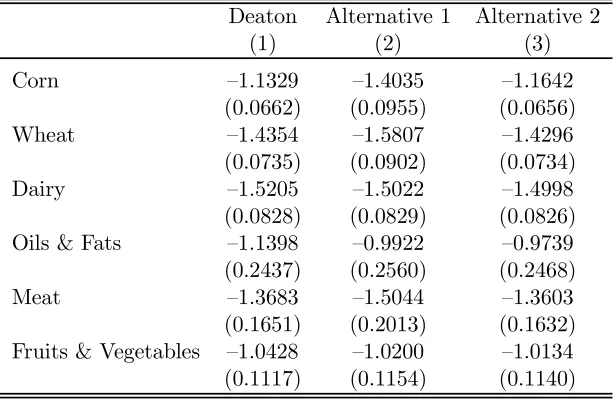
In Table A2.2, I report the own-price elasticities estimated with the special case of section 3.1. Essentially the same results are obtained. Notice that thefirst column reports the results that would be obtained using Deaton (1990) method.
Table A2.2 Own-price Elasticities Young Adults Labor Model
Deaton Alternative 1 Alternative 2 (1) (2) (3) Corn —1.1329 —1.4035 —1.1642
(0.0662) (0.0955) (0.0656) Wheat —1.4354 —1.5807 —1.4296 (0.0735) (0.0902) (0.0734) Dairy —1.5205 —1.5022 —1.4998 (0.0828) (0.0829) (0.0826) Oils & Fats —1.1398 —0.9922 —0.9739 (0.2437) (0.2560) (0.2468) Meat —1.3683 —1.5044 —1.3603 (0.1651) (0.2013) (0.1632) Fruits & Vegetables —1.0428 —1.0200 —1.0134 (0.1117) (0.1154) (0.1140)
(1) Estimation using Deaton’s (1990) formulas (2) Alternative 1: Ψe =I
(3) Alternative 2: Ψ˜ =D(vecdiag(Ψe))
Table A2.3 Cross-price Elasticities
Full Model with Instrumental Variables
Oils & Fruits & Corn Wheat Dairy
Fats Meat Vegetables Corn -0.9995 0.0192 -0.0768 -0.2667 -0.1276 0.2066
(0.0541) (0.0603) (0.1442) (0.0858) (0.0615) (0.0482) Wheat 0.1376 -1.3121 0.1154 0.3258 0.1061 -0.0875
(0.0695) (0.0643) (0.1268) (0.1050) (0.0670) (0.0611) Dairy 0.4665 0.1304 -1.8857 -0.4092 0.4292 0.4311
(0.0672) (0.0592) (0.1175) (0.0901) (0.0678) (0.0462) Oils & Fats 0.0676 -0.7266 -0.1182 -1.1240 0.0114 0.5746
(0.2370) (0.2216) (0.5054) (0.3232) (0.3293) (0.1719) Meat -0.1803 0.1386 0.0579 -0.1858 -1.1785 0.3661
(0.1007) (0.0929) (0.2011) (0.1435) (0.1347) (0.0733) Fruits & Vegetables -0.0868 -0.0273 -0.0470 0.0425 0.1709 -0.9472
(0.1413) (0.1407) (0.3074) (0.2185) (0.1613) (0.1134)
[image:27.612.97.518.475.669.2]References
Balat, J. and G. Porto (2004). “Occupational Choices and Trade Reforms: Informality, Self
Employment and WTO Reforms,” mimeo World Bank.
Benjamin, D. (1992). “Household Composition, Labor Markets, and Labor Demand: Testing
for Separation in Agricultural Household Models,”Econometrica, vol. 60, No.2, pp. 287-322.
Deaton, A. (1987). “Estimation of Own- and Cross-Price Elasticities From Household Survey
Data,”Journal of Econometrics, vol. 36, pp. 7-30.
Deaton, A. (1988). “Quality, Quantity, and Spatial Variation of Price,”American Economic
Review, vol. 78 No 3, pp. 418-430.
Deaton, A. (1990). “Price Elasticities from Survey Data,” Journal of Econometrics, vol. 44,
pp. 281-309.
Deaton, A. (1997). The Analysis of Household Surveys. A Microeconometric Approach to
Development Policy, John Hopkins University Press for the World Bank.
Deaton, A. and J. Muellbauer (1980). Economics and Consumer Behavior, Cambridge
University Press.
Deaton, A. and J. Muellbauer (1980). “An Almost Ideal Demand System,” American
Economic Review, vol 70, pp. 312-336.
Dixit, A. and V. Norman (1980).Theory of International Trade. A Dual, General Equilibrium
Approach, Cambridge Economic Handbooks.
Edmonds, E. and N. Pavcnik (2003). “The Effects of Trade Liberalization on Child Labor,”
mimeo, Dartmouth College.
Edmonds, E. and N. Pavcnik (2004). “Trade Liberalization and Household Labor Supply in
Feenstra, R. C. (2004). Advanced International Trade: Theory and Evidence, Princeton
University Press, Princeton.
Goldberg, P. and N. Pavcnik (2003). “The Response of the Informal Sector to Trade
Liberalization,” Journal of Development Economics, forthcoming.
Goldberg, L. and J. Tracy (2003). “Exchange Rates and Wages,” Federal Reserve Bank of
New York, mimeo.
Hsiao, C. (1986). Analysis of Panel Data, Econometric Society Monographs No 11,
Cambridge University Press.
Kloek, T. (1981). “OLS Estimation in a Model Where a Microvariable is Explained by
Aggregates and Contemporaneuos Disturbances are Equicorrelated,”Econometrica, vol. 49,
No1, pp. 205-207.
Leamer, E. E. (1996). “In Search of Stolper-Samuelson Effects on US Wages,” NBER
WP5427.
Porto, G. (2003). “Using Survey Data to Assess the The Distributional Effects of Trade
Policies,” Policy Research Working paper, the World Bank Research Group.
Porto, G. (2004). “Agricultural Trade Reforms, Wages and Unemployment,” mimeo, World
Bank Research Group.
Ravallion, M. (1990). “Rural Welfare Effects of Food Price Changes Under Induced Wage
Responses: Theory and Evidence for Bangladesh,” Oxford Economic Papers, vol. 42, pp.
574-585.
Rosenbaim, P. R., and D. B. Rubin (1983). “The Central Role of the Propensity Score in
Observational Studies for Causal Effects,” Biometrika, 70, pp. 41-55.
Singh, I., L. Squire, and J. Strauss, eds. (1985).Agricultural Household Models: Extensions,
Wolak, F. A. (1996). “The Welfare Impacts of Competitive Telecommunications Supply:
A Household-Level Analysis,”Brookings Papers on Economic Activity Microeconomics, vol.