4-(N2-1) puzzle: parallelization and performance on clusters

4-(

N

2

_{-1) Puzzle: Parallelization and performance on clusters}

Victoria Sanz

III LIDI, Facultad de Informática, Universidad Nacional de La Plata La Plata, Buenos Aires, Argentina

and

Armando De Giusti

III LIDI, Facultad de Informática, Universidad Nacional de La Plata La Plata, Buenos Aires, Argentina

and Marcelo Naiouf

III LIDI, Facultad de Informática, Universidad Nacional de La Plata La Plata, Buenos Aires, Argentina

ABSTRACT

In this paper, an analysis of the 4-(N2_{-1) Puzzle, which is a} generalization of the (N2-1) Puzzle, is presented. This problem is of interest due to its algorithmic and computational complexity and its applications to robot movements with several objectives.

Taking the formal definition as a starting point, 4 heuristics that can be used to predict the best achievable objective and to estimate the number of steps required to reach a solution state from a given configuration are analyzed. By selecting the objective, a sequential and parallel solution over a cluster is presented for the (N2-1) Puzzle, based on the heuristic search algorithm A*. Also, variations of the classic heuristic are analyzed.

The experimental work focuses on analyzing the possible superlinearity and the scalability of the parallel solution on clusters, by varying the physical configuration and the dimension of the problem.

Finally, the suitability of the heuristic used to assess the best achievable objective in the 4-(N2_{-1) Puzzle is} analyzed.

Keywords: Multi-objective problems, discrete optimization, superlinearity, parallel algorithms.

1 INTRODUCTION

One of the areas of interest in parallel computing in recent years has been search processing in graphs. Discrete optimization problems (DOP) comprise a large number of areas [1] and are often solved with search algorithms that

browse the state space of the problem to reach a “solution”

state that minimizes a target function [2].

In general, these search techniques have a high computational cost because state spaces grow in a factorial or exponential manner. Oftentimes it is impossible to perform a thorough analysis of the solution space, so algorithms that use heuristics are required to assess the cost of the states and process first the nodes that are most likely to yield the best results [3] [4].

The high computational complexity as regards computational time and memory requirements are drivers for the development of parallel algorithms for discrete optimization problems to achieve an efficient solution; in particular, graph processing techniques to represent the problem have been of great interest [5] [6].

This is the case of some variations of the BFS (Best First Search) search method, which start from a node of the graph representing the problem to solve and apply some type of work assessment metrics to reach a solution,

so as to evolve from an initial state of the graph towards

the “optimum solution” state.

The natural parallelization of the technique consists in

starting the evolution from different “possible” nodes on

the different processors of the multiprocessor architecture. As the algorithm progresses, processors need to be communicated to be able to report the partial results achieved and enable search termination detection or discard solutions that, based on the selected metrics, will not improve the partial solution found so far [7] [8].

Some of the aspects observed when using cluster-type parallel architectures for the resolution of discrete optimization problems [9] are of interest:

▪

Parallelization granularity (ratio between independent processing time and communication) is critical for performance, since it will affect the improvement of solution time as well as communications overhead.

▪

In general, load balancing has to be dynamic, since the state space is implicit and generated during the search. This requires communication, since exploratory work is variable and very hard to predict a priori [10]. In parallel processing, two of the main aspects of performance analysis are the Speedup factor (Sp) [11] [12] and the Efficiency (E) that relates the Speedup with the number of processors (N) used [13] [14].

Scalability is a third, very significant factor in parallel applications: problems usually scale, i.e., by increasing the volume of work to be done, and the multiprocessor architectures used can also scale by increasing the number of processors used. The effect of escalating workload and/or processors on the performance of parallel algorithms, considering Sp and E [15], is of interest.

The maximum theoretical speedup can in some cases be improved, which is known as superlinearity (Su). The reasons why the Sp can be greater than N, in particular for discrete optimization problems, is an issue of interest:

▪

The exploration of the total space of possible solutions can be reduced by distributing the workload between N

processors so as to “cut down” or “finish” the global

search when reaching the expected result in any of these processors [16] [17]. That is, in theory, the cluster architecture will allow superlinearity depending on workload balancing, processor heterogeneity, and the processing time/communication time ratio of the algorithm used [18].

time imposes a limit on the possibility of obtaining superlinearity [19].

2 CONTRIBUTION

In this paper, a multi-objective generalization of the (N2_-1) Puzzle is presented and its application to robot movement planning is analyzed [20]. The contributions are:

▪

Analyzing time improvements in the sequential and parallel algorithms presented in [21] achieved with the application of variations in prediction heuristics that combine Manhattan Distance (DM) and Linear Conflict Detection (CL) with the detection of the last movements carried out to solve the board and the location of corner tiles.

▪

Carrying out experimental work based on these algorithms with boards of various dimensions and clusters of 4, 8, 12, and 16 processors, varying heuristics and analyzing the performance obtained in each case.

▪

Analyzing a local work parameter (LW) that is related to load balancing and is used during the execution of the parallel algorithm.

▪

Analyzing the suitability of the heuristic used to assess the best achievable objective in the 4-(N2-1) Puzzle.

3 4-(N2-1) PUZZLE: GENERALIZATION OF THE (N2-1) PUZZLE TO MULTIPLE

OBJECTIVES

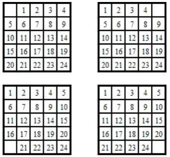
[image:2.595.97.268.411.568.2]

The 4-(N2-1) Puzzle is an extension of the (N2-1) Puzzle, applicable in multi-objective robot movements. It has the following characteristics:

Fig. 1. Solution boards for the general problem.

▪

Given an initial board, 4 possible solutions are

admitted, each of these being a “target board”. In

Figure 1 these solutions are shown for N = 5. Once the target is chosen, the problem becomes that of solving the (N2-1) Puzzle, the final board being the selected target.

▪

The analysis of solvable cases for a target board is that presented in Section 4.1, and it will be different for the achievable “target boards” if N is an even or an odd number.

4 CHARACTERIZATION OF THE (N2-1) PUZZLE The (N2-1) Puzzle problem is a generalization of the Puzzle-15 [22]. It consists in N2-1 pieces numbered from 1 to N2-1 and placed on a N2-sized board. Each square of the

board contains one piece, so there is only one empty square. Figure 2 shows the (N2-1) Puzzle with N = 4.

▪

A legal movement implies moving the empty square to an adjacent position, either horizontally or vertically, by moving the piece that was in the newly emptied square to the previous position of the empty square.

▪

The objective of the Puzzle is applying legal movements until the initial board becomes the selected final board (Figure 2). The solution to the problem should be the one that minimizes the number of movements required to achieve the final configuration from the initial given configuration.

Fig. 2. Boards for the 15 (N=4) Puzzle. a. Initial board. b. Final board.

4.1 Solvability of the Puzzle

The state space of the (N2-1) Puzzle has N2! states. However, not every state can be reached from any other state by applying legal movements. This is because the graph representing the state space of the Puzzle has two equally-sized connected components, and therefore, if the initial and the final states are not in the same component, there is no solution for the problem.

By applying a simple detection step prior to the search process, in order to determine if the final configuration can be reached from the initial configuration, the state space of the (N2-1) Puzzle is reduced to N2!/2.

The procedure to corroborate if an initial board can be solved into a final board is the following:

▪

For each piece i (i = 2..N2

-1), the number of pieces with a lower number that appear after the piece in question – whether on the same row to the right or on any lower row – are counted. We will call this the “i inversion

number”, and will denote it as ni.

▪

Then, NT = n2 + n3+… n(N2-1) is calculated for both the initial and final boards. If N is an even number, the number of the row where the empty square is located is added to NT.

▪

If the parity of both results is the same, then the final board can be reached from the initial board. This is because (NT mod 2) does not vary with any legal movement.

Figure 2 shows an example for an even N, where the board in 2.a has NT = 28 and the board in 2.b has NT=4; therefore the board in Figure 2.a can be solved into that final board.

4.2 Heuristics

A more polished heuristic will carry out estimates that are closer to the real cost; therefore, the algorithms that use it will need to process less nodes.

The heuristics used for the implementation of the sequential and parallel algorithms are: (H1) addition of Manhattan Distances, (H2) H1+ detection of Linear Conflicts, (H3) H2+ Last Movements, (H4) H3+ Corner Tiles. The corresponding definitions can be found in [23].

In this paper, the best heuristic (H4) is used for the 4-(N2-1) Puzzle in order to estimate the most easily reachable objective (lowest number of steps to reach the solution), and its suitability is determined.

5 SEQUENTIAL SOLUTION

A* is a variation of the Best First Search search technique [6], where each node n is valuated in accordance to the cost of reaching it from the root of the search tree (g(n)) and a heuristic that estimates the cost to go from n to the solution node (h(n)). Thus, the cost function will be f(n) =

g(n) + h(n). If the heuristic is admissible, i.e., it never overestimates the real cost, the algorithm A* will always find the best solution.

The algorithm keeps a list of unexplored nodes (open list1) ordered by the value of function f, and a second list of already explored nodes (closed list2) used to avoid loops in the search graph. Initially, the open list contains only one element, the initial node, and the closed list is empty.

After each step, the node with the lowest f value (the most promising node) is removed from the open list and examined. If the node is the solution, the algorithm ends. Otherwise, the node is expanded (generating the children nodes by applying legal movements) and added to the closed list. Each successive node is added to the open list if it has not been previously processed or if it has been processed but its cost value improves the previous one.

In order to check time improvement as the heuristic is tuned, tests with 60 initial configurations were carried out varying the heuristic function (H1, H2, H3, H4). In most cases (65%), the heuristic H4 produced the best execution times, followed by H3 (20%), and H2 (15%). In general, it was noted that, as the heuristic is adjusted, running time, the number of processed and exploited nodes, and the average size of the lists of the structure used as closed list (factor LPLC) decrease.

6 OUTLINE OF THE PARALLEL SOLUTION The parallelization strategy consists in keeping local open and closed lists on each processor. At the beginning, only one of the processors will work with the initial node, and it will also be in charge of detecting the end of the search. As other nodes are generated, processors will receive them and start working.

All processors will search locally, building their own closed list – to avoid locally repeated work – as well as their open list. Processors should communicate among them the minimum values of the solutions found in order to minimize unnecessary searches.

Since the graph for the problem is implicit and generated during the execution, a dynamic load balancing technique has to be adopted. These strategies are based on

1 _{The open and closed lists are implemented by means of a}

priority queue and a hash table, respectively.

2 _{The open and closed lists are implemented by means of a}

priority queue and a hash table, respectively.

the idle processor selecting a work donor process. If the latter has work, it sends part of its load to the requesting process. Otherwise, it sends a rejection message, and the idle process looks for another donor. The technique used in the algorithm is the Asynchronous Round Robin [11]. The quality of the nodes sent has to be considered as well, since, if the nodes sent are known not to lead to a better solution, then the receiver will quickly become idle.

To detect the end of the search in a distributed environment with a dynamic load balancing technique, the

modified Dijkstra’s Termination Algorithm [24] is used, whose purpose is detecting the state in which processes are idle and there are no messages circulating through the network. To this end, processes are connected in a ring structure and pass a message called token between them.

A global pruning algorithm was used where each of the

p“worker” processes has a value that indicates the cost of

the best solution found so far (BSC), which is used to limit the search process. Thus, the nodes to process will be only those whose cost is lower than BSC.

A process that has some work pending on its open list will process at the most a fixed amount of nodes for each iteration (LW), or it will process nodes until it finds a

solution or until its open list is empty. Then, the “worker”

receives the costs of the “best solutions” – if there are any

– found so far by the other workers and updates its BSC

variable as needed.

If the process still has some work pending on its open list, it checks if there are any work requests from other processes, and if there are, it sends the first and last nodes of its open list to the requesting processor. It then continues working with its nodes.

If the process does not have any pending work, it will be idle, so it will send a work request to its donor following the ARR algorithm. If the process found a new solution, it sends the corresponding cost to the other processes. It then waits for the types of messages listed below, which will be processed with no particular order of priority:

▪

Work request: an idle worker selected this process as its donor.

▪

Work: the donor sends the requested work. The process is active again.

▪

Rejection of work request: the selected donor does not have any work. The process must send a work request message to the next donor.

▪

Token: reception of the token for termination detection. If necessary, the token is updated and the next process begins. Process 0, upon receiving the token, checks if it has to end the search process and, if that is the case, it sends a message to the other processes to inform the end of the computation.

▪

New solution found: if necessary, the BSC variable is updated.

The termination token is used to translate the minimum cost solution movements to process 0, so that the messages communicating new solutions only have a value (cost) to avoid communication overhead.

7 EXPERIMENTAL RESULTS

For the tests, a cluster of 20 Pentium IV, 2.4 GHz, and 1GB RAM computers connected over a 100-Mbit LAN was used.

LW parameter (500, 750, 1000). For each initial configuration, the sequential algorithm was run with the different heuristics (since the speedup has to be taken based on the best sequential algorithm). In 65 % of the tests, superlinear results were obtained.

One cause for superlinearity occurs when, during parallel execution, a solution node is reached after examining a lower number of nodes than the sequential algorithm. In BFS algorithms, this anomaly is caused by nodes that have the exact same cost. Another cause is the reduction of the LPLC factor in each processor. Since work is distributed among processors, each closed list is smaller and therefore the search processes for the elimination of cycles are faster, which means that it is more likely to be enough memory for them.

To see how the algorithm escalates as the size of the problem increases (N = 4, 5, 6) and as the number of processors in the architecture escalates (P = 4, 8, 12, 16), two types of initial configuration were defined, created based on: (1) inversion of the third column and the third row of the lower right 4x4 sub-board (Figure 3.a), (2) inversion of the second column and the second row of the lower right 4x4 sub-board (Figure 3.b). The solution to be found will be based on the classic solution board.

Fig. 3. Examples of 5x5 boards. a. Configuration 1 b. Configuration 2.

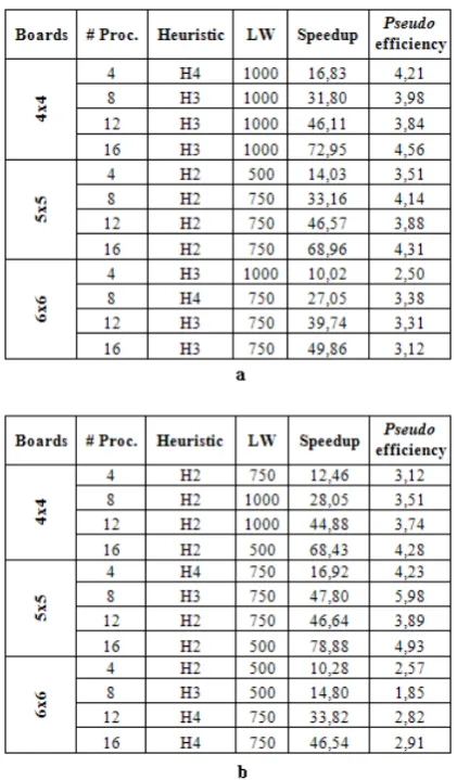
For each configuration and each P, the LW block size (500, 750, 1000) that optimizes times was looked for. The best times for each configuration are shown in Figures 4.a and 4.b, respectively.

Based on these results, it can be seen that, as P

increases, for a specific N and configuration, the speedup increases as well. Therefore, efficiency first increases and then decreases when the number of machines increases, or it remains more or less at the same level. Also, when N

increases, the speedup decreases. This may be due to two reasons:

▪

The state space grows exponentially as N increases, which results in an increase of the nodes expanded by the algorithm.

▪

Each work request communication will require sending a larger volume of data because the boards are bigger. The role of the LW parameter, presented in Section 6, should be noted. It measures the number of nodes to

process at each “worker” by iteration of the algorithm

before checking work requests received and examining partial solutions found by other processors.

A large value of LW might cause idle processors waiting to receive work to remain in this state for a long time. Also, since the costs of sub-optimum solutions found by others would not be received, unnecessary nodes would be processed. A very small value of LW would allow more frequent checks, but it might cause an increase of times due to the constant verifications.

Fig. 4. Best parallel times. a. Configuration 1 b. Configuration 2.

During the tests carried out, it was observed that there is no optimum LW value – it depends on the dynamic distribution of the state space. For example, if the processors have a tendency to run out of work, a smaller value of LW will be more suitable, so that the processors that are selected as donors can answer the request from the idle processor.

With the purpose of analyzing the suitability of the heuristic H4 for the 4-(N2-1) Puzzle, each initial board was run with the two objectives that were closest as regards the initial disorder so as to calculate the number of steps required to reach the solution. The two remaining objectives were discarded because their initial disorder is above the number of steps corresponding to the solutions of the other two objectives.

The results obtained were classified based on:

▪

Successful: the objective selected with the heuristic H4 is reached in a lower number of steps.

There was a 67% rate of Successful results.

▪

Unsuccessful: the objective discarded by the heuristic H4 is reached in a lower number of steps.

There was an 8% rate of Unsuccessful results.

▪

The cases for which H4 indicates that both objectives are equivalent were not considered.

[image:4.595.311.522.68.428.2] [image:4.595.95.268.327.416.2]

number of steps between the two objectives is N-1 steps.

8 CONCLUSIONS AND FUTURE LINES OF WORK

A generalization (4(N2-1) Puzzle) of the (N2-1) Puzzle has been defined, particularly useful for some cases of robot movement planning.

Four heuristics that can be used both to predict the best reachable objective and to estimate the number of steps

required to reach a “solution” state from a given

configuration have been analyzed.

An analysis of the parallel solution for the (N2-1) Puzzle on clusters has been presented, incorporating the implementation of variations of the classic heuristic. The advantages of using these variations for the sequential and the parallel algorithms has been analyzed, and speedup, efficiency and superlinearity factors have been analyzed for various cluster configurations, various problem dimensions, and various initial states.

One research line that is currently being studied is the migration of the algorithm to multicore and multicore cluster platforms. The strategy in this case would be taking into account those workers that are inside the same cluster node and having an only open and closed list for them. Another research line currently under study is the parallelization of the multiple-objective problem increasing to M the number of boards to solve.

9 REFERENCES

[1] Sergienko I., Shylo V. Problems of discrete optimization: Challenges and main approaches to solve them. New York: Springer; 2006; 42(4):465-482.

[2] Lambur H, Shaw B. Parallel State Space Searching Algorithms. 2004.

www.metablake.com/parallel_search_project [3] Grama A., Kumar V. State of the art in parallel search

techniques for discrete optimization problems. IEEE Trans. on Knowledge and Data Engineering, 1999. [4] Parberry I. A Real Time Algorithm for the (n2-1)

Puzzle. Information Processing Letters 1995;56(1): 23-28.

[5] Ferreira A., Pardalos P. Solving Combinatorial Optimization Problems in Parallel: Methods and Techniques. New York: Springer; 1996.

[6] Reinefeld A. Complete Solution of the Eight-Puzzle and the Benefit of Node Ordering in IDA*. In: Proc. of the 13th International Joint Conference on Artificial Intelligence; Chambery Savoi, France; 1993. p. 248-253.

[7] Hanson O., Mayer A., Yung M. Criticizing Solutions to Relaxed Model Yields Powerful Admissible Heuristics. Information Sciences 1992; 63(3): 207-227.

[8] Korf R. E., Schultze P. Large-scale parallel breadth-first search. In: Proc. of the 20th National Conference on Artificial Intelligence; Pittsburgh, USA; 2005. p. 1380-1385.

[9] Anderson T., Culler D., Patterson D. A Case for NOW (Networks of Workstations). IEEE Micro 1995; 15(1): pp. 54-64.

[10]Bohn C., Lamont G. Load Balancing for Heterogeneous Clusters of PCs. Future Generation Computer Systems, 2002; 18(3): 389-400.

[11]Grama A., Gupta A., Karypis G., Kumar V. An Introduction to Parallel Computing. Design and Analysis of Algorithms. Pearson Addison Wesley; 2003.

[12]Leopold C. Parallel and distributed computing. A survey of models, paradigms, and approaches. New York: Wiley; 2001.

[13]Quiin M. J. Parallel Computing: Theory and Practice. McGraw-Hill Companies; 1993.

[14]Buyya R. High Performance Cluster Computing: Architectures and Systems. Prentice-Hall; 1999. [15]Hwang K. Advanced Computer Architecture.

Parallelism, Scalability, Programmability. McGraw Hill; 1993.

[16]Helmbold D., McDowell C. Modeling speedup(n) greater than n. IEEE Trans. on Parallel and Distributed Systems, 1990; 1(2): 250-256.

[17]Manquinho V., Marques-Silva J. Search Pruning Techniques in SAT-Branch-and-Bound Algorithms for Binate Covering Problem. IEEE Trans. on Computer-Aided Design of Integrated Circuits and Systems, 2002; 21(5): 505-516.

[18]Sanz V., Chichizola F., Naiouf M., De Giusti L.,De Giusti A. Superlinealidad sobre Clusters. Análisis experimental en el problema del Puzzle N2-1. In: Proc. of the XIII Congreso Argentino de Ciencias de la Computación; Chaco-Corrientes, Argentina; 2007. p. 1300-1309.

[19]Wilkinson B., Allien M. Parallel Programming: Techniques and Applications Using Network Workstation and Parallel Computers. Pearson Prentice Hall; 2005.

[20]Fitch R., Butler Z., Rus D. Reconfiguration Planning Among Obstacles for Heterogeneous Self-Reconfiguring Robots. In: Proc. of the IEEE International Conference on Robotics and Automation; 2005. p. 117-124.

[21]Sanz V., Chichizola F., De Giusti A, Naiouf M, De Giusti L. Análisis de Performance en el procesamiento paralelo sobre Clusters del problema del Puzzle N2-1. ENIEF 2008. XVII Congreso sobre Métodos Numéricos y sus Aplicaciones. ISSN: 1666-6070

[22]Ratner D. and Warmuth W. Finding a shortest solution for the NxN extension of the 15-Puzzle is intractable. AAAI-86, 168-172

[23]Sanz V. Paralelización de problemas de búsqueda en grafos en una arquitectura tipo cluster. Análisis de Performance. Informe Final de Trabajo de Grado; 2009.