The long and winding road towards fiscal decentralization

Keywords: Decentralization, default, taxes, sub-national governments. THE LONG AND WINDING ROAD TOWARDS FISCAL

DECENTRALIZATION

MARÍA LAURA ALZÚA AND CAROLINA LOPEZ

RESUMEN

Este trabajo ofrece una explicación teórica de las dificultades asociadas en un proceso de descentralización fiscal desde gobiernos nacionales a sub-nacionales, como es observado en numerosos países en desarrollo. Un marco teórico de juegos es usado para mostrar que la escasez del gobierno central de un compromiso tecnológico creíble, usado para penalizar el despilfarro fiscal de los gobiernos sub-nacionales, puede dar lugar a un nivel incompleto de descentralización fiscal. Dos diferentes conjuntos de equilibrios son obtenidos. En uno de ellos el gobierno central le conferirá completa autonomía fiscal a los gobiernos sub-nacionales, mientras que en el otro el gobierno mantiene la autoridad fiscal ya que es óptimo hacerlo. En este caso la economía cae en un nivel ineficiente de descentralización fiscal, medido en términos de recaudación de ingresos.

Clasificación JEL: E62, H63, H72

Palabras Clave: Descentralización, cesasión de pagos, impuestos, gobiernos

subnacionales.

ABSTRACT

This paper o_ffers a theoretical explanation of the di_fficulties embodied in a

process of fiscal decentralization from national to sub-national governments, as it is empirically observed in numerous developing countries. A game theoretic

framework is used to show that the central government’s lack of a credible

commitment technology, used to penalize sub-national governments’ fiscal profligacy, may give rise to an incomplete level of fiscal decentralization. Two di_fferent sets of equilibria are obtained. In one of them the central government will confer complete taxing autonomy to the sub-national governments, while in the other the government maintains the taxing authority since it is optimal to do so. In this case, the economy falls in an inefficient level of fiscal

THE LONG AND WINDING ROAD TOWARDS FISCAL DECENTRALIZATION

MARÍA LAURA ALZÚA AND CAROLINA LOPEZ*

I. Introduction

One of the main recent institutional innovations for developing countries is that of fiscal decentralization of decision making authorities to sub-national governments, both in terms of the provision of public goods and revenue collection. The most widespread approach to decentralization in the public finance literature is known as fiscal federalism. It identifies three main functions for the public sector in terms of public spending: macroeconomic stabilization, income redistribution and resource allocation.

While macroeconomic stabilization and income redistribution functions are assigned to the cen- tral government, sub-national governments should be in charge of resource allocation mainly for efficiency reasons. It is argued that while some public goods such as national defense confer benefits to the whole nation, some other goods such as garbage collection, basic education, etc. are more limited in geographical incidence. In such cases, by making decisions concerning the provision and financing of such goods at sub-national government's level, an optimal level of provision can be achieved. In a decentralized setting, sub-national governments choose the “mix" of taxes and

public goods they consume according to their citizens' preferences.

Recent history of developing countries shows serious intents of central governments to pursue fiscal decentralization both for efficiency reasons and as ways to induce fiscal discipline in lower level of governments. International organizations also advocate for such decentralization. For example, as stated in the Policy Statement on IMF technical assistance, one of the core activities of the organization's assistance in the area of fiscal affairs is to collaborate with

“the design of structural policy reforms, and related institutional reforms, for

sustainable revenue mobilization, including macro-significant inter-jurisdictional issues (e.g. fi_{scal federalism, tariff reform)”}.

In spite of the efficiency reason stated above, effective decentralization rests on institutional structures that may not exist when a process of fiscal decentralization starts and it may take time to build such institutions. There is not much research, both at the theoretical and empirical level, addressing the problems that arise during a decentralization process or analyzing whether such process would produce useful results. Among many of the issues which deserve attention in order to engage in a process of fiscal decentralization we can mention the timing of decentralization and the conditions under which such process can be optimally concluded.

As mentioned above, a large number of developing countries - Latin American countries, African and Eastern European countries - are undergoing processes of fiscal decentralization. Whereas each country presents differences in such processes, one particular feature observed in many of them is the decentralization of some public expenditures without the corresponding decentralization of revenues. Moreover, some other elements that are often required in order to attain a successful decentralization may not be present in these countries. Among them, we can mention: the state of the system of intergovernmental grants between different levels of governments, sub-national governments' capacity to raise taxes and the type of budget constraint faced by sub-national governments.

Regarding the issue of intergovernmental grants, its design is crucial at the moment of decentralization, since some of these systems may induce irresponsible fiscal behavior on behalf of lower levels of governments. If, for example, lower levels of government rely too much on intergovernmental grants in order to finance decentralized expenditures, then individuals enjoying the benefit of consuming public goods may not bear the total cost of providing

them. This is known as “lack of fiscal correspondence". Furthermore, if

bureaucracy operating at lower level of governments is not as efficient as that of the national government. To sum up, each process of fiscal decentralization may have different outcomes resulting from the different institutional structures mentioned above.

The present study is aimed at analyzing which are the different economic configurations that may give rise to a sub-optimal level of decentralization in a federal country. In order to match the stylized fact that decentralization of expenditures comes before revenue decentralization, we look at an economy where expenditure autonomy has already been granted to sub-national governments, but revenues are still collected at the national level.

We develop a model to study the interaction of a Central Government, henceforth CG, and Regional or Sub-national Governments (RGs) in the

context of a real economy. We model two different situations: first, one economy which has random endowments. We look for the Equilibrium of the game between CG and one RG. CG has to decide whether to grant taxing

autonomy to the regions or not. We look for the Weak Perfect Bayesian Equilibrium, restricting ourselves to pure strategies. We obtain different sets of equilibria. There are different configurations of parameters which support different choices for each level of government. Choices will depend on parameters like endowment volatility, size of the region, default and decentralization costs.

We are interested in looking at the set of beliefs and strategies that give rise to the regional taxation equilibrium and to the equilibrium without fiscal decentralization. The former is the most efficient in terms of the decentralization theorem and reduces the deficit bias observed in regional governments. The latter is of interest since many of the countries undergoing decentralization fall into this intermediate phase of fiscal decentralization; it is worth looking at which configuration of parameters give rise to this equilibrium. Secondly, we repeat the game allowing for regional interaction. We look for the Sub-game Perfect Nash Equilibrium, since as we will show, random output plays no restrictions on beliefs, and so, in order to simplify the inter-regional game, we eliminated it. Again there are different sets of equilibria: one with complete fiscal decentralization and the other with no taxing autonomy.

over output. Section 4 extends the game to allow interaction between RGs and

the CG. Section 5 provides some explanation of why the model could be

applied to Argentina and other developing countries and some policy implications. Finally, Section 6 concludes.

II. Literature Review

The present section presents a summary of two main issues concerning fiscal federalism. The first one is a brief mention to normative aspects of decentralization. The second one refers to the problems generally associated to fiscal decentralization which are related to the model developed later in the chapter.

The main issues concerning normative aspects of fiscal federalism are surveyed by Oates (1999). He reviews the different aspects to be considered in the evolution of fiscal federalism theory: how to assign the different expenditure and revenue raising functions to the different level of governments, which are the gains from fiscal decentralization in terms of efficiency, and how to use fiscal instruments (taxes and debt). Finally he mentions some recent developments on the field of political economy of fiscal federalism, and fiscal decentralization in developing and transitional economies as well.

Classical theory of fiscal federalism (Musgrave, 1959) states normative functions for the different level of governments. While Federal Government should be responsible for macroeconomic stabilization and income redistribution, lower level of governments must take care in the provision of public goods whose consumption is limited to their jurisdictions. Oates (1972) states the Decentralization Theorem, justifying the local provision of public

goods based on efficiency reasons: “...in the absence of cost savings from the

centralized provision of a (local public) good and interjurisdiccional externalities, the level of welfare will always be at least as high (and typically higher) if Paretto efficient level of consumption are provided in each jurisdiction than if any single, uniform level of consumption is maintained across all jurisdictions".

Oates (1998) provides evidence of the welfare gains arising from fiscal decentralization.

Another point of relevance for fiscal federalism theory is how to raise taxes in order to finance public expenditures and which is the structure of revenue raising responsibilities best suited for a decentralized provision of public goods. Gordon (1983) presents evidence of distortions originated by decentralization of taxes without taking into account the effects of fiscal decisions in different jurisdictions (such as exporting tax burden, congestion effects, etc.). He presents some normative principles for the use of different taxes by different level of governments.

Another topic often addressed by fiscal federalism literature is that of intergovernmental grants, since they may serve different policy objectives. Gordon (1983), Feldstein (1975) and Inman and Rubinfeld (1979) discuss several aspects of intergovernmental transfers: whether they may serve the purpose of correcting distortions, equalizing taxable capacity and transferring income from richer to poorer areas. Bradford and Oates (1971) state a prescriptive theory of intergovernmental grants where benefit spillovers across jurisdictions, revenue sharing and income redistribution are taken into account. McKinnon (1997) explores the relationship between decentralization and a growing economy and the importance of having subnational governments facing hard budget constraints and full separation of monetary and fiscal powers. As McKinnon states, a hard budget constraint means that lower level of governments must rely in their own sources of revenues in order to finance their expenditures.

which allow them to reduce the dependence of transfers from higher levels of governments. Finally, the federal government must ensure that the decentralized governments face restrictions to debt financing to avoid the use of such instruments to cover large deficits.

While existing literature on fiscal federalism provides some insight on normative issues like efficiency gains from decentralization, tax assignments between the different level of governments, etc. there is much less work done on the problem associated with engaging in fiscal decentralization processes in developing countries. Tanzi (2000) makes a good account of the hurdles that may appear as a consequence of decentralization such as: the size of the country, how regulations will change after decentralization, corruption at lower level of governments, tax and expenditures assignment, difficulties for tax reforms, macroeconomic coordination, regional disparities, timing of decentralization and quality of lower levels of government's public employment. He stresses the need to further study these issues before recommending deepening decentralization processes in developing countries. He finally concludes that in some cases it may not even be such a good policy recommendation.

Narrowing down the literature to problems associated to fiscally decentralized countries we mention two pieces of work from which the model developed later builds on. One refers to the timing of decentralization and the other to the bailout mechanisms behind RG’s and CG interaction. As far as the

timing of decentralization is concerned, Garcia Mila and McGuire (2001) develop a model to explore the more frequently observed sequence for decentralization: decentralization of expenditures followed by tax decentralization. They test their model for Spain and find evidence that there might be inefficient regional borrowing (sub-national governments borrowing

“too much" from central government) resulting from this timing for

decentralization.

Incentives for regional borrowing depend on the regions' expectations about how the federal system of finances is going to evolve. Their results suggest that if taxing authority is given back to the regions, then sub-national borrowing can efficiently correct any initial revenue deficiency. But, if regional governments expect the central government to increase grants as a response to the increase in regional borrowing, then a “soft budget constraint"

Qian and Weingast (1997) find that in a context of fiscal federalism and, to the extent that lower level of governments do not have access to a central bank

to bail them out, they will be facing a “hard budget constraint". However, if

they gain indirect access to the central bank through intergovernmental transfers, then, their budget constraints are softened.

Cooper et al. (2005) study the different repayment paths of regional debt issued by members of a federation. They found that if CG is able to commit

not to bailout RGs, then the former will use its taxation power to smooth

distortionary taxes across regions. Without commitment CG will bailout RGs

to smooth consumption and distortionary taxes across regions. These two solutions result in different welfare implications.

Among the approaches to fiscal federalism we can consider the Second Generation Fiscal federalism (SGFF) based on the first generation (which considers only benevolent planners who seek to maximize the welfare of society, ignoring the objectives of permanence in office). The second generation models deal specifically on the importance of political parties and how regional governments act to protect their power from the central government, and the importance of democratic systems, among others (Weingast, 2013). In this paper we focus on first generation model, the model we develop in the next sections builds on some aspects of both Garcia Mila and McGuire (2001) and Cooper et al. (2005). Two further features have been added: strategic action between CG and RGs and the modeling CG bailout vs. taxing decisions.

The model developed can be applied to di_fferent developing countries

engaged in processes of fiscal decentralization. We focuse on Argentina, in

1989-1990 the country suffered two episodes of hyperinflation and sank into

macroeconomic stagnation. In 1991 a newly elected government launched a program of deep structural reforms. Among the most important reforms we can mention a currency board which pegged the domestic currency (Argentine peso) to the US dollar together with a law (called Convertibility Law) which prevented the Central Bank from issuing domestic money if it was not backed by foreign reserves. Money supply depended on the amount of reserves in the hand of the Central Bank. In this sense, the currency board eliminated the

“inflation tax”, but this mechanism was soon replaced by issuing debt,

exchange rate regime prevents the government from printing money to finance its deficits. In this sense, one of the results of adopting a currency board is that it acted as implicit hardening of the budget constraint. Given the structure of all level governments in Argentina, Convertibility meant that the CG should

introduce reforms outcome after the monetary one. The fiscal reform rested on

two pillars: prohibition of financing in the tax system and in government expenditures. In this sense, the fiscal reform was an expected deficits by

printing money (derived directly by the restrictions of the Currency Board) and the beginning of a process of fiscal decentralization, giving back decision

power to RGs. At the time of decentralization, the main pro-decentralization

reasons were efficiency and a way to induce fiscal discipline in RGs, given that CG monetary bailouts would no longer be possible. The country moved fast in

terms of expenditure decentralization, but faced harder challenges when attempted tax reforms. Revenue collection is still highly centralized. Basically,

CG collects most of the taxes and redistributes back to RGs through a

complicated tax-sharing agreement of intergovernmental grants called

“Coparticipacion Federal de Impuestos”. This creates a severe vertical

imbalance problem (as it can be observed in Table 1), which was often followed in the past by several GB bailout episodes, not financed by issuing

money but debt. This imbalance is unequal and becomes very high for some provinces (like fomosa, Corrientes, Santiago del Estero) reaching 80% of provincial revenues (Ardanaz et al., 2013).

As mentioned above, while the reform program succeeded in reducing

inflation, it was not able to achieve fiscal discipline (at least at the sub-national level). This indiscipline caused great indebtedness and forced the central government to abandon the peg and to default on its debt.

Saiegh and Tommasi (1999) state that the two most important problems in

Argentina’s fiscal structure are the lack of fiscal correspondence between sub -national revenues and expenditures and the central government recurrent bailouts of sub-national units. First of all, there is a lack of fiscal

borrowing autonomy. However, taxes are still heavily centralized at the national government. Taxes are collected by the Central Government (CG) and

then re-distributed in the form of transfers to the provinces (RG) through a

system called “Coparticipacion Federal” (tax-sharing agreement). Provinces di_ffer in both share of the national income and in population. The tax-sharing agreement as it is today presents two main drawbacks:

1. The unit of redistribution of CG revenues is the region and not the

households. This has been historically the case since governors of the di_fferent regions give their support to the CG. The power of each governor in the Upper

house of the Congress does not bear any relationship with the population or share of income of the di_fferent regions. So bigger regions are under-represented and smaller regions are over-under-represented. As a consequence, per capita transfers di_ffer widely across regions.

2. The second problem is derived directly from the first one, and it is the

deficit bias that this way of sharing transfers creates. For bigger and wealthier

provinces (wealthier in terms of higher share of income, not in terms of per

capita income), the incentive to run deficits is too big: they create most of the

taxable income of the country and they are not able to reap its benefits Similarly, poorer regions do not have any incentives to reduce their deficits either. In this case, any fiscally responsible region will receive fewer transfers than its fiscally irresponsible neighbor. But, regardless of the wealth or the

regions, there is a lack of fiscal correspondence between the benefit of

enjoying public goods and the cost to provide them. Moreover, the fact that

RGs have borrowing autonomy makes matters even worse, since many

provinces generally run large deficits, borrow abroad and then wait for the CG

to bail them out.

Provinces collect few taxes, and on average provincial expenditure is financed only by one-third of own resources of each province. According to political or economic circumstances, during the last decades the federal government has discretionaryly allocated funds to the provinces, despite the provisions of the Ley Federal de Coparticipación (Ardanaz et al, 2013).

III. A Game between CG and one RG

We develop a simple two period model to study a real endowment economy. The country is undergoing a process of fiscal decentralization, expenditures are decentralized at a regional level but revenues are still centralized at the national level. The economy is populated by N identical agents who live for two periods. There is a CG and two regional governments

(RG1 and RG2). Population in each region is N1 and N2, respectively, they may

not necessarily be equal and Δ and (1 - _{Δ) are the population shares of e}ach region. Individuals cannot move from one region to the other. Agents have endowments in both periods. Individuals live for two periods where the

superscripts “y” and “o” will stand for young and old respectively.

While there is certainty in period one endowment, period two endowment is random, but perfectly correlated across regions, and takes the value high (Y h)

with probability p and low (Y l) with probability (1-p)1. Expenditure policy is

determined at the regional level. In period one CG makes g transfers to the

provinces. Following Mila et al. (2000) we consider the transfers of period one to be exogenous and assume that there is a mismatch between g, and RG

spending in this period in order to introduce RG's borrowing or lending as in

McGuire et al. (2001).

We are going to assume that only RG1 is active and issues debt, while there

is no mismatch between CG grants and RG'2s expenditures. This can be

thought of, for example, RG2 having borrowing restrictions in its constitution.

The timing of the game is as follows: Stage one:

 CG sets exogenous transfers to the provinces and decentralizes

expenditures.

 RGs issue bonds 1

j

b _{, j = 1; 2, to finance the gap between CG’s transfers and}

desired spending. Debt can be held in either region, and the superscript j

indicates the region were debt is held.

 All young agents make decisions in anticipation of period two government policies.

At stage two, CG and RG play the following game which can be observed

in the tree below:

 Regional governments observe the realization of endowments Yh or Yl, high

and low endowment respectively.

 CG decides to give taxing authority (TA) to RG or not (NTA).

 If CG gives taxing authority to RGs, RGs can choose to levi the tax (T) by

charging individuals of Region 1 a proportional tax 1 on endowments or pass the obligation to the CG (NT).

 CG can choose to bail out (BO) RGs by means of an economy wide tax

proportional to regional per capita endowments.

 If CG does not levi an economy-wide tax, RGs will default (D), paying a

penalty cost δ.

 If CG does not pass the taxing authority (NTA) to RGs then it pays off RG'1sdebt by means of an economy wide tax proportional to regional per

capita endowments.

We search for a Weak Perfect Bayesian Equilibria (WPBE) of this game, restricting ourselves to pure strategies. CG cannot make credible threats not to

bail out RG1. We will analyze the equilibria when the CG lacks this

commitment power.

The solution for the first period optimization problem and for CG-RG1

game with a complete derivation of the payoffs can be found in Appendix A.

III.1. Payoffs

In period one, agents in each region solve a standard maximization problem deciding consumption (of a public, giy and

o i

g _{, and a private good} y i

c _{i and} o i

c

) and Region 1 debt holdings bi1.

Agents are able to smooth private and public good consumption, achieving intertemporal efficiency, but, due to the lack of regional taxation in period one, intratemporal efficiency is not achieved. Issuing regional debt does not correct for initial mis-funding of regional governments.2

In the second period, there is a game played by CG and RG1. Each government has different payoffs according to their welfare functions.

While RG1 maximizes second period per capita consumption for their citizens, CG has to optimize a welfare function that includes a population

weighted average of per capita consumption for the second period and an autonomous consumption for CG, .

We can write the welfare function of CG as follows:

1 (1 ) 2

CG o o

W     c c    ₍₁₎

 _{is a parameter which captures the cost of a bailout. This parameter can be}

understood as an “extra effort" on behalf of the Central Government once it has given taxing autonomy to the regions. We are going to consider  as fixed, but in a more complicated environment, it can be made a function of  , the tax rate: the higher the tax rate, the higher the reduction in CG consumption; or a

function of the population shares, since the bigger the region the more costly is a bailout. For the CG, the welfare of a CG bailout will then decrease, the

higher the level of regional debt.3

While CG does not know the realization of endowments when deciding

whether to grant taxing autonomy, RG does. The rationale for this comes from

2 _{This is the same result obtained in Garcia Mila and McGuire (2001).}

the fact that in general RGs possesses much more information about the

productivity and the real possibilities of their economies than the CG. A

principal agent problem arises, where it is costly for the CG to monitor the

activity in the regions.

III.2. Equilibria

We look for the Weak Perfect Bayesian Equilibrium (WPBE),4 restricting ourselves to pure strategies. As mentioned before, we obtain different sets of equilibria. There are different configurations of parameters which support different choices for each level of government. We are interested in looking at the set of beliefs and strategies that give rise to the taxing autonomy-regional taxation equilibrium and to the equilibrium without fiscal decentralization. The former is the most efficient in terms of the decentralization theorem and reduces the deficit bias observed in regional governments. The latter is of interest since many of the countries undergoing decentralization processes may stay in this intermediate phase of fiscal decentralization, with a problem of

“vertical imbalance" and CG’s bailouts.

3.2.1 Equilibrium with fiscal decentralization and regional taxation

Proposition1.Under the following condition5  

  ₍₂₎

there exists an equilibrium where CG grants taxing autonomy to RG1 and RG1 taxes its citizens.

Intuitively, this equilibria will be supported for high bailout costs -high  - which lowers CG autonomous consumption.6 The smaller the size of the

region ∆, the higher the range of values within which this equilibrium will be

supported, since the welfare function of CG is a population weighted average

4 _{Please refer to Appendix A for a detailed analysis of equilibria.} 5 _{The proof of this proposition appears in the Appendix.}

of second period consumption. Finally, small default costs  relative to  increase the feasibility of this equilibrium. This fact looks a little counterintuitive, since it is sometimes suggested by the literature that increasing default costs may induce sub-national government discipline. Here what matters is and its relationship to  , and not its absolute value.

It is interesting to note that output volatility does not matter for the CG

decision to grant taxing autonomy or not. Output volatility matters only to the decision of RG whether to tax or not once taxing autonomy has been conceded.

1

( )

E R b  _{ }  _



  _{defines the maximum level of debt which can ∆ be held in}

equilibrium in each region).

3.2.2 Equilibrium without fiscal decentralization

Proposition 2.Under the following condition7  

  ₍₃₎

there exists an equilibrium where CG will not give taxing autonomy to RG1 .

Here CG always prefers not to grant taxing autonomy regardless of p.

Again, output volatility plays no role in CG decision. Low decentralization

costs make a CG bailout after taxing autonomy has been granted more

attractive, and so CG prefers not to give taxing autonomy in the first place.

There are no restrictions on CG beliefs for which CG will prefer a bailout

to a default. It only depends on the fiscal cost of a bailout  with respect to the default costs in CG’s government function. This also depends on R1

population, since allowing default is more costly the bigger R1 is. Given that CG always bailout R1, then it is always the case than RG1 will not choose

regional taxation, regardless of output realization. Here regional tax e_ffort is non-existent and complete fiscal decentralization will never take place.

This equilibrium is easily supported the higher the size of R1 (∆) and the

higher default costs  . Ex-post consumption for individuals living in R1 is

higher than for the ones in R2. This is because they get to repay less than in the

case of regional taxation, since the tax is spread between the two regions.

IV. A game of regional interaction

While the simple model presented in the previous section where only one region is active sheds some light about why a country may end up in a process

of incomplete fiscal decentralization, it is useful to study what happens when

regional interaction is taken into account, since it is a more accurate representation of what happens in decentralized countries.

Here we present a model where two regions (RG1 and RG2) interact while CG must decide whether to grant taxing autonomy to regional governments. In

order to simplify the game studied we eliminate output volatility, since we showed it played no major role in CG decision. Otherwise the model is the

same than the one developed in the previous section. The timing of the game is as follows:

Stage one:

• CG sets exogenous transfers to the regions and decentralizes expenditures.

• RGs issue bonds bi to finance the gap between CG’s transfers and desired spending.

• All young agents make decisions in anticipation of period two government

policies.

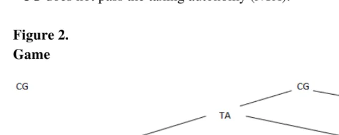
In stage two, CG and RGs play the following game, the corresponding tree

can be observed below:

• CG decides to give taxing autonomy (TA) to RGs or not (NTA).

• If CG gives taxing autonomy to RGs, RGs play a simultaneous move game

where they can choose to levy a regional tax i (_T) or pass the obligation to the CG (NT).

• CG can choose to bail out (BO) RGs by means of an economy wide tax .

• If CG does not levy an economy wide tax, RGs will default (D), paying a

• CG does not pass the taxing autonomy (NTA).

Figure 2. Game

We search for a Sub-game Perfect Nash Equilibria (SPNE) of this game. The CG cannot make credible threats not to bail out RGs. We will analyze the

equilibria when the CG lacks this commitment power.

IV.1. Payoffs

The period 1 optimization problem is analogous to the one with one region, but there is no uncertainty and now individuals can hold bonds of either region.

In the second period, payo_ffs are also derived similarly to the single region case. The welfare functions of CG and RG1 remain the same. Now, we add RG2, whose welfare function corresponds to per capita consumption of its

citizens in the second period. The solutions to the maximization problem and to the second period game appear in Appendix B.

IV.2. Equilibria

the equilibrium with complete fiscal decentralization and to the one where CG

keeps its taxing autonomy.

4.2.1 Equilibrium with fiscal decentralization and regional taxation

Proposition3.Under the following condition:

  ₍₄₎

there exists an equilibrium where CG will give taxing autonomy to RGs and RGs will tax its citizens.

As in the case in which only one region is active, this payo_ff corresponds to

the state where complete fiscal decentralization is achieved. This is the “good equilibrium” in terms of the decentralization theorem. Here each region will

bear the full cost of repaying period one debt by taxing its citizens.

As in the one region model, the equilibrium with taxing autonomy depends on the size of the regions and default costs relative to bailout costs. However,

the condition is more restrictive than in the single region case, since ∆ < 1 for a

given .

4.2.2 Equilibrium without fiscal decentralization

Proposition 4.Under any of the following conditions:

, (1 ) ,

        ₍₅₎

, (1 ) ,

        ₍₆₎

, (1 ) ,

        ₍₇₎

there exists an equilibrium where CG will not give taxing autonomy to RGs.

CG will not grant taxing autonomy in the following:

case a)

, (1 ) ,

For this configuration of parameters NTA CG BO. Here default costs are high relatively to the loss in CG welfare caused by the NTA option. Fiscal

decentralization is not complete. Thus, CG always prefer a bailout to a default

once they grant taxing autonomy, so the no taxing autonomy alternative will

be chosen in the first place.

case b)

, (1 ) ,

       

In this case, CG will proceed to a bailout whenever RGs play (NT, NT), and

whenever RG1 does not tax.

However, even when CG would allow default in R1, this will not happen,

since R1 incentives are to deviate and play No Tax, since CG will bail both

regions out. Here NTA CG TA. case c)

, (1 ) ,

       

This case is symmetric to b), but R2 is the region where default will be

allowed. Again both regions will play (NT, NT), andNTA CG TA.

One interesting point in cases b) and c) is that while in each of the cases there are incentives for one region to tax, knowing that a bailout is feasible in the event of the other region default, the region where default will be allowed ends up being bailed out as well. This result provides support for the moral behavior of RGs. As long as CG will bailout one region, then none of the

regions will choose taxation, even when they have incentives to do so.

V. An application to Argentina and some policy implications

The model developed in the previous section can be applied to di_fferent

developing countries engaged in processes of fiscal decentralization. In what

follows we will take a close look to the Argentine case, since the country underwent a process of fiscal decentralization together with a program where

CG gave up the management of monetary policy. In the past fifty years,

Argentina presented a long history of fiscal indiscipline, with large bailouts to

RGs financed using the “inflation tax”. For example, the “inflation tax”

accelerated by the late eighties, there was clear political consensus that this

way of deficit financing had to be be ended.

The models presented before can be applied to the Argentine economy with

some caveats. For example, the population weights ∆ and (1 − ∆) in CG’s welfare function are not representative for Argentina, due to the fact that CG,

for political reasons redistributes resources across regions according to other factors di_fferent from population. In Argentina, CG often needs governors’

support in Congress, so in terms of transfers to the provinces it is often the case that per capita transfers are higher in low densely populated provinces. Currently, the tax sharing regime is based on the following weights, 65% on population, 10% according to demographic dispersion and 25% according to

the development gap, defined as the difference between each province wealth with respect to the richest one.

With regards to the parameter , we can mention one interesting example

of this “extra tax effort” on behalf of the CG. In 1994, the Social Security

System was privatized at the national level but some provinces kept the old PAYG system. Given that CG abandoned the state-funded PAYG system, the

amount of instruments in the hands of the CG available to bailout regions was

reduced. CG had to resort to borrowing, which resulted in an accumulation of

an unsustainable level of debt.

As regards to CG transfers to RGs, past expenditure decentralization in

Argentina has been an attempt to begin to improve the problem of resource allocation from the point of view of expenditures. But the main drawback of such process has been the impossibility of achieving some degree of tax decentralization. CG has lost control over expenditure decisions -making any

adjustment more di_fficult- and, at the same time it must raise revenues in order

to finance sub-national expenditures. The transfers to sub-national governments are automatically guaranteed by the Tax Sharing Agreement, which poses a burden on Central Government accounts. Any economic

downturn complicates the fiscal solvency of the Central Government, since it

has to provide funds to the regional units with little flexibility in expenditure.

As far as bailouts from CG are concerned, as Nicolini et. al. (2002)

conclude:

were associated with jurisdic- tions running very unsustainable fiscal policies that at some point moved the province into almost bankruptcy”.

Finally, it is worth mentioning the last episode of CG bailout. Before the

abandoning of the Convertibility, the RG had issued “monies” worth $6

billion. In 2002-2003 the CG bailed out the provinces by absorbing their debt

once again.

At this point, we will point out some policy implications that can be drawn directly from the model presented. Among them we can mention: limits to regional debt, structure of debt return and default costs.8

If issuing debt is not allowed for RGs, then the problem of bailout episodes

disappears. But this solution is hard to implement in a context of federal countries, since many times Regional Governments existed before the country was constituted and had their own constitutions.

Also, debt allows regions to achieve intertemporal e_fficiency in consumption, which will not happen if the regions are forced not to issue debt. Some countries (Switzerland and Norway for example) have limits for their sub-national governments as to what they can finance by issuing debt, for

example, it is not possible to finance current expenditures. Debt issuing is used instead to finance infrastructure projects, where the benefits are enjoyed and

paid not only by the current but by future generations.

Increasing default costs have two opposite e_ffects. On one hand, they reduce the attractiveness of RG’s default with respect to the costs of regional taxation. But, on the other hand, they increase CG incentives for a bailout in

the first place, unless the region we are considering is su_fficiently small.

V. Conclusions

The advocacy towards fiscal decentralization both in the provision of public

goods and in revenue collection is a prevalent policy recommendation across international institutions. Many developing countries and transition economies are engaged in such processes, but so far and to di_fferent extents, some countries have failed in achieving an efficient level of fiscal decentralization, either because the vertical imbalance is worsened, consolidated fiscal deficit

increases, bailout episodes become more frequent or even the quality of public goods provided deteriorates in some regions.

It is often the case that some central governments find it very difficult to discipline sub-national governments and thus, the implementation of complete

fiscal decentralization may not happen. We developed two very simple models

in a game theoretic framework to analyze interactions between a regional and a central government and then we allow regions to interact with the central government. Our results suggest that according to di_fferent parameter

configurations we can obtain two sets of equilibria, one where complete fiscal

decentralization is achieved and a second one, where it is not. Contrary to our priors, endowment volatility played no role on central government beliefs. In

the first case, where only one region is active, the model can be understood as

follows: CG is mechanism used by RGs to pass to each other tax pressure to

finance their expenditure levels, here, only from RG1 to RG2.

The di_fferent sets of equilibria obtained will have di_fferent welfare implications for the individuals in each region. The equilibrium with regional taxation would be the one preferred by individuals in Region 2, while individuals in Region 1 prefer to be bailed out by the Central Government. As it was mentioned before there are different parameter configurations that matter for the choice of equilibrium. The first of them is regional size, since

the Central Government weights each region according to its population: the bigger Region 1 is, the lower the range of parameters for which the Central Government will give taxing autonomy. Finally, debt holding distributions should be taken into account, since any legal limitation to the holding of debt outside the region or debt caps to regional debt will also work in this direction. When we allow for regional interaction, our results do not change

significantly. There are still different parameter configurations which sustain

an equilibrium with decentralization and another one without it. The interesting addition is that even in the case where the central government will

allow default for one specific region, such region has an incentive to deviate

from taxing, since the central government will proceed to a bailout if both

regions default. In this sense, it corroborates the idea of existence of “moral hazard”, as long as CG is willing to bailout one region.

Among the many extensions which can be considered, we will mention some for future work. The assumption that R is exogenous can be too strong,

be extended to a multiregional context, and with different specification of welfare functions for the Central Government. As far as the sequence of the game is stated, we made no comment as to why CG starts by decentralizing

expenditures first; we model it in that way since it is the most common trend

observed in practice. Probably, it is due to political reasons that decentralization evolves in this way. Here we take the sequence as given.

Also, the model can be modified to allow for monetary policy aiming at

studying welfare implications of a central government bailout by means of an

inflation tax. In the models we have presented, there is no difference between a nation-wide tax and an inflation tax, but the model can become more

sophisticated by allowing some regional or agent heterogeneity with di_fferent welfare e_ffects between the two options for bailout.

References

Ardanaz, M., M. Leiras and M. Tommasi (2013). "The Politics of Federalism in Argentina and its Implications for Governance and Accountability." World Development, in press.

Bird, R. and F. Vaillancourt (1998). Fiscal Decentralization in Developing Countries. Cambridge, New York and Melbourne: Cambridge University

Press.

Bradford, D. and W. Oates (1971). "Towards a Predictive Theory if Intergovernmental Grants." American Economic Review, Papers and

Proceedings of the Eighty-Third Annual Meeting of the American Economic Association, Vol. 61(2): 440-448.

Campbell, T. (2001). The Quiet Revolution: The Rise of Political Participation on Leading Cities with decentralization in Latin American and the Caribbean.

Pittsburgh: University of Pittsburgh Press.

Feldstein, M. (1975). "Wealth Neutrality and Local Choice in Public Education." American Economic Review, Vol. 65(1): 75-89.

Garcia-Milà, T. and T. McGuire (2001). "Do Interregional Transfers Improve the Economic Performance of Poor Regions? The Case of Spain." International Tax and Public Finance, Vol. 8(3): 281-296.

Gordon, R. (1983). "An Optimal Taxation Approach to Fiscal Federalism."

The Quarterly Journal of Economics, Vol. 98: 567-586.

Musgrave, R. (1959). The Theory of Public Finance. New York: McGraw Hill.

McKinnon, R. (1997). "EMU as a Device for Collective Fiscal Retrenchment." The American Economic Review Paper and Proceedings of the Hundred and Fourth Annual Meeting of the American Economic Association 87, pp. 227-229.

Oates, W. (1972). Fiscal Federalism.New York: Hartcourt Brace Jovanovich.

Oates, W. (1985). "Searching for Leviathan: An Empirical Study." American Economic Review, Vol. 75( 4): 748-757.

Oates, W. (1998). "On the Welfare Gains from Fiscal Decentralization."

Oates, W. (1999). "An Essay on Fiscal Federalism." Journal of Economic Literature, Vol.37: 1120-1149

Qian, Y. and B. Weingast (1997). "Federalism as a Commitment to Preserving Market Incentives." Journal of Economic Perspectives, Vol.11: 83-92.

Saiegh, S. and M. Tommasi (1999). "Why is Argentina’s Fiscal Federalism so

Inefficient? Entering the Labyrinth." Journal of Applied Economics Vol. 2(1):

169-209.

Shah, A. (1997). "Fiscal Federalism and Macroeconomic Governance: For Better or for Worse?" Mimeo, World Bank.

Tiebout, C. (1956). "A Pure Theory of Local Expenditures." The Journal of Political Economy, Vol. 64( 5): 416-424.

Appendix A

1. Game with no regional interaction

A.1 Period 1 Optimization

Individuals derive utility from consumption of a private and public good. Region i young agents solve:









,

max , ,

i i i j

y y o o

i i i i

b b

u c g Eu c g

  

 

(8)

for i = 1, 2 where u is assumed to be concave, subject to:

y i y

i i

c b Y ₍₉₎

y y

i i

g g b ₍₁₀₎





( ) 1 ( )

o o

i i i i

c E R b     E Y

(11)

( ) ( )

o y o

i i i i

g g E R b E Y T ₍₁₂₎

i j

i i i

b b b ₍₁₃₎

where all the variables are expressed in per capita terms. gy is real transfer

when young to agents on region i, go is real transfer when old to agents on

region i, Yiy is endowment when young, ( ) o i

E Y _{, random endowment when}

old, bi _{is debt held in region i,} j i

b _{is debt issued in region i and held in region}

j, i is a regional tax and is a common tax collected by CG,











 2_{1 1} 1 ₂

t Y Y

T



are total tax revenues and ∆ and (1 − ∆) are

population shares of R1 and R2 respectively.

R is the return on regional debt and is considered to be exogenous9 taking

two values: Rh when output is high and Rl= αRh, with 0 < α < 1.

9 _{In our simple setting we just consider}

R to be exogenous but positively correlated with

Given some initial conditions, this maximization problem is well defined

and has explicit solutions for consumption and regional government debt holdings for some parametrical assumptions about the utility functions.

The first order conditions for this problem are:

( ) : '( )i y '( )y ( '( ))o ( '( ))y

i i i i i

b u c u g 



(14)

( ) : '( )j y ( '( ))o

i i i

b u c  



(15)

The left hand side of (14) is the marginal cost of giving up consumption today. In this sense, increasing public good consumption reduces this marginal cost. The right hand side represents the marginal benefit of consumption

tomorrow. From (14) and (15) we obtain:

'( )y ( '( ))y

i i

u g  



(16)

and

'( ) '( )

( )

( '( )) ( '( ))

y y

i i

o o

i i

u c u g

E R

E u c  E u g  ₍₁₇₎

(17) is the standard intertemporal e_fficiency relationship between present and future consumption for private and public goods. Here, agents are able to smooth private and public good consumption, achieving intertemporal e_fficiency, but, due to the lack of regional taxation in period one, intratem- poral e_fficiency is not achieved. Issuing regional debt does not correct for initial mis-funding of regional governments.10

A.2 Period 2 payo_ffs

In order to consider the second period payo_ffs we make some simplifying

assumptions. First, we A.2 assume a linear utility function u c

 

automatic transfers in period two will be equal to zero.

As mentioned in the text, the second period payo_ffs are regional consumption and population weighed consumption for RG and CG

respectively.

A.2.1 CG gives taxing autonomy and RG1 taxes its citizens.

This payo_ffcorresponds to the state where complete fiscal decentralization is achieved. This is the “good equilibrium” in terms of the decentralization

theorem. Here R1 individuals will bear the full cost of repaying period one

debt. This equilibrium will be the one “preferred” by R2 individuals.

The payo_ffs when endowments are high correspond to:

2

(1 ) 1

b

RG o h

h

W c  Y R _{ and}

WCG= Π + Yh , which are the welfare functions

of the regional and central government respectively.

Similarly, we can derive the payo_ffs when endowments are low,

2

(1 ) 1

b

RG o h

t

W c  Y



WCG= Π+Yt. When endowments are low, return

on regional debt is Rl = αRh . The parameter α ranges between zero and one

and it is the default rate, i.e. a low realization of endowment means partial

default on period one government debt. If α = 1, debt can still be repaid when

endowment is low. Incomplete information on behalf of the CG plays no role in determining the di_fferent equilibrium of the game. By introducing default risk, we will be able to look at two di_fferent things: the role of endowment volatility as a parameter that a_ffects the result of the game and the role of informational asymmetries between CG and RG, in the sense that the latter

knows the state of the economy before than the former.

Regardless of the realization of endowments, ex-post consumption in R1 is

lower the higher the proportion of debt held in R2 . R1 individuals bear the tax

burden to repay the debt held in R2. This will produce an analogous result to

the one found in Cooper et. al. (2003), where they find an equilibrium with

regional taxation when debt is held just in R1 .

A.2.2 CG gives taxing autonomy, RG1 does not levi a regional tax, and CG

bails out RG by means of higher economy-wide taxes.

Payo_ffs when endowment is high are

2

(1 )b

RG h

h

W AY R _{ , where}

(1 )

1

A_    _ 

Payo_ffs when endowment is low are

2

(1 )b

RG h

t

W AY 



WCG= Π

− γ+ Yl.

We are assuming that CG charges an uniform tax rate in both regions.

Here, A is greater than one, so payoff for the RG1 will be higher than in the

case of regional taxation regardless of the level of b2. This seems reasonable,

since RG2 citizens bear also the burden of higher taxation in period two. This

result will be preferred by RG1 citizens, since they can enjoy higher

consumption in period one and share the burden of re-paying debt with R2

individuals. CG has the above mentioned cost γ, due to the fact that it has

already given taxing authority to the regions, and so bailouts entail a higher e_ffort that lowers CG autonomous consumption.

A.2.3 CG gives taxing autonomy, RG1 does not levi a regional tax, and CG

allows default.

Payo_ffs when endowment is high are: WRG = Yh − δ and W

CG_{= Π − ∆δ + Y} h_.

Payo_ffs when endowment is low: WRG = Yl − δ and W

CG_{= Π − ∆δ + Y} l.

A.2.4 CG does not give taxing autonomy

Here, the fiscal decentralization process is not complete. Regions do not enjoy taxing autonomy, so the process of fiscal imbalance may worsen. This creates deficit biases in region 1.

Payo_ffs when endowments are high are

2

(1 )b

RG h

h

W AY R _{ and W}CG₌

Π+Yh_{. Payo}

ffs when endowment is low are

2

(1 )b

RG h

t

W AY 



Π+Yl_.

A.3 Equilibria

In order to define a Weak Perfect Bayesian Equilibrium we must define a set of strategies and system of beliefs ( , µ) such that is sequentially rational

given the system of beliefs µ and the system of beliefs µ is derived from

strategy profile through Bayes’ rule whenever possible.

Γ=Γ(CG,RG)={[(TA,BO), (T,T)], [(TA,BO), (T,NT)], [(TA,BO), (NT,T)],

[(TA,BO), (NT,NT)], [(TA,D), (T,T)], [(TA,D), (T,NT], [(TA,D), (NT,T)], [(TA,D), (NT,NT)], [NTA,-i]}

where i is any action taken by RG1 .

A.3.1 Last Stage of the Game

CG will prefer BO to D for the following sets of beliefs:

( h ) (1 )( ) ( h ) (1 )( )

CG l l

BO D  Y      Y   Y         Y 

which requires γ < ∆δ, with no restrictions on CGs beliefs.

If γ <∆δ, there are no restrictions on beliefs, and CG will always prefer to

bail out the regions than to allow default. As γ increases, a bailout becomes

more costly in terms of CG welfare. This also will depend on the size of R1 and

the technology that penalizes default. Note than here, increasing default costs,

increases the set of values of γ for which CG will prefer a bailout. Also, there

are no restrictions on beliefs µ, so output volatility does not matter in order for

the CG to choose a course of action.

A.3.2 Second Stage of the Game

RG1 has the following strategies for each realization of endowment: (T,T), (T,NT), (NT,NT), (NT,T)

a)     BO CGD

a.1. Left node: NT RGT, whenever (1 − ∆) ≥ 0, which is always the case.

RG will always choose no regional taxation.

a.2. Right node: NT RGT , whenever (1 − ∆) ≥ 0, which is always the case.

RG will always choose no regional taxation as in the left node. Here again,

output volatility plays no role in the set of strategies that is chosen.

Whenever RG1 knows CG will proceed to a bailout, then, they will never

choose to tax its citizens, since by a bailout RG1 can pass the cost of repaying RG1 debt to R2 individuals. This means higher consumption for R2 agents in the

second period.

b.1. Left node NT RGT , whenever

2

1 h

R b  _{ }  _



  _(*)

b.2. Right node: NT RGT, satisfied whenever

2

1 h

R b  _{ }  _



  _(**).

Default costs δ which satisfy (**), will also satisfy (*), since α < 1. If, (*)

holds but (**) does not, then RG will choose taxation in the bad realization of endowment but no taxation when endowments are high. This seems a little counterintuitive, since one would expect that the lower realization of output would induce the RGto be more inclined towards a bailout. This depends on α.

When α is small, then the tax e_ffort in terms of output is low, so consumption will increase with regional taxation relative to default. By increasing default costs, the set for which (*) holds is reduced, but the probability of a CG bailout

increases. Unless the loss in welfare γ for CG is too high, then increasing

default costs have this potential harmful e_ffect in terms of regional taxation.

A.3.3 First Stage

a)     BO CG D, and NT RGT, under (1 − ∆) ≥ 0, NTA CGTAis always preferred regardless of p. Here, output volatility plays no role in

deciding whether CG will give taxing autonomy or not. Given that CG will

bailout RG, then it prefers not to grant TA in the first place, increasing CG

welfare by gamma.

Appendix B

1. Game with regional interaction

B.1 Period 1 Optimization

Individuals derive utility from consumption of a private and public good. Region i young agents solve:



 







i o i y i y i b b

g

c

u

g

c

u

,

,

max

,





for i = 1, 2 where u is assumed to be concave, subject to:

y i

i i

c b Y ₍₁₉₎

y y

i i

g g b ₍₂₀₎





o

i i i i

c Rb     Y

(21)

o y

i i i i i

g g Rb Y T ₍₂₂₎

i j

i i i

b b b ₍₂₃₎

where all the variables are expressed in per capita terms, and the same

notation than in the one region case applies, with the exception that here, η1 =

∆ and η2 = (1 − ∆)11, which means whenever CG collects an economy wide tax, it redistributes back according to each region population. R is the return on

holding regional Government debt, and is considered to be exogenous.

Again, given some initial conditions, this maximization problem is well

defined and has explicit solutions for consumption and regional government debt holdings for some parametrical assumptions about the utility functions.

The first order conditions for this problem are:

11 _{We can analyze the case of different η}

( ) : '( )i y '( y) ( '( )) (o '( y))

i i i i i

b u c u g  Ru c  Ru g ₍₂₄₎

( ) : '( )j y '( )o

i i i

b u c  



(25)

The left hand side of (24) is the marginal cost of giving up consumption today. In this sense, increasing public good consumption reduces this marginal

cost. The right hand side represents the marginal benefit of consumption tomorrow. From (24) and (25) we obtain:

'( )y '( )y

i i

u g  



(26)

and

'( ) '( )

'( ) '( )

y y

i i

o o

i i

u c u g

R

u c u g  ₍₂₇₎

with the same implications than in the one region case, where, due to the lack of regional taxation in period one, intratemporal e_fficiency is not achieved. Issuing regional debt does not correct for initial mis-funding of regional governments.

B.2 Period 2 payo_ffs

In order to consider the second period payo_ffs we make the same assumptions than in the one region case. First, we will assume a linear utility function as in the one region case u(cy) = cy and go = 0, which means that in

equilibrium,

b



b



b



b



b

1 1 2 1

1 _.12

Finally, CG transfers in period two will be equal to zero. RG1 and RG2

governments are concerned with the welfare of its citizens, their welfare function equals consumption in the second period. We will assume the same welfare function for the CG than in the previous case:





CG

1 2

W   c 1 o    c o    

(28)

Also, we will assume that γ is constant regarding whether CG has to bailout

one of both regions. The results do not change if we allow γ being region -population weighted and output is the same for both regions, their only difference being population size. τur final assumption is that if CG is