SERIE DO C UM ENTO S DE TRA BA JO
No . 8 5
Julio 2 0 1 0
ON BLAME-FREENESS AND RECIPROCITY: AN EXPERIMENTAL
STUDY
O
n
B
lame
-
freeness and
R
eciprocity
: A
n
E
xperimental
S
tudy
∗M
ariana
B
lanco
†Universidad delRosario
B
o ˘gaçhan
Ç
elen
‡ColumbiaUniversity
A
ndrew
S
chotter
§NewYorkUniversity
June28, 2010
Abstract
The theory of reciprocity is predicated on the assumption that people are willing to reward nice or kind acts and to punish unkind ones. This assumption raises
the question as to how to define kindness. In this paper we offer a new definition
of kindness that we call “blame-freeness.” Put most simply, blame-freeness states
that in judging whether player i has been kind or unkind to player j in a social
situation, player j would have to put himself in the strategic position of player i,
while retaining his preferences, and ask if he would have acted in a manner that
was worse thanidid under identical circumstances. If jwould have acted in a more
unkind manner thaniacted, then we say that jdoes not blameifor his behavior. If,
however, j would have been nicer than iwas, then we say that “jblames i” for his
actions (i’s actions were blameworthy). We consider this notion a natural, intuitive
and empirically relevant way to explain the motives of people engaged in reciprocal behavior. After developing the conceptual framework, we then test this concept in a laboratory experiment involving tournaments and find significant support for the theory.
JEL ClassificationNumbers: A13, C72, D63.
Keywords: Altruism, blame, reciprocity.
∗We are grateful to participants in the CESS Experimental Economics Lunchtime Seminar, 2009
North-American ESA Conference, the Amsterdam Workshop on Behavioral & Experimental Economics, and seminars at Cornell University and the Brown University for comments. We also acknowledge the partial financial support of the Center for Experimental Social Science at NYU. The findings, recommendations, interpretations and conclusions expressed in this paper are those of the authors and not necessarily reflect the view of the Department of Economics of the Universidad del Rosario.
†Faculdad de Economía, Universidad del Rosario, Calle 14 # 4-80, Oficina 207, Bogóta, Colombia.
E-mail: [email protected], url: http://mbnet26.googlepages.com/home/.
‡C.E.S.S., New York University, and Graduate School of Business, Columbia University, 3022 Broadway,
602 Uris Hall, New York, NY 10027. E-mail:[email protected], url: http://celen.gsb.columbia.edu/. §C.E.S.S. and Department of Economics, New York University, 19 W. 4th Street, New York, NY 10012.
1
Introduction
Recent years have witnessed a growing literature on the theory of reciprocity. Founded
on the seminal work of Rabin [18]—further extended by Falk and Fischbacher [10],
Dufwenberg and Kirschteiger [5] and others, and generalized by Sobel and Segal [21]—
the theory of reciprocity is predicated on the assumption that people are willing to
re-ward nice or kind acts and to punish unkind ones.1 This assumption raises the question
of as to how to define “kindness.” In this paper we offer a definition of kindness that we call blame-freeness. The notion that we propose is a natural, intuitive and empiri-cally relevant way to explain the motives of people engaged in reciprocal behavior. We develop the conceptual framework and then test it in a laboratory experiment involving tournaments.
Put most simply, blame-freeness states that in judging whether playerihas been kind
or unkind to player jin a social situation, playerjwould have to put himself in the
strate-gic position of player i, while retaining intrinsic characteristics of his preferences (i.e., j
does not become i but simply takes his strategic position), and ask if he would have
acted in a manner that was worse than i did under identical circumstances. If j would
have acted in a more unkind manner thaniacted, then we say that jdoes not blameifor
his behavior. If, however, jwould have been nicer thani was, then we say that “jblames
i” for his actions—i.e. i’s actions were blameworthy. Furthermore, if blame is a source
of disutility, j may have the motivation to punish i whenever possible even if the
pun-ishment is costly for him. Note that blameworthiness is only a necessary condition for punishment while blame-freeness is a sufficient condition for non-punishment. In other words, in the strong form of the theory, we should never observe any player punishing those whose actions are judged blame-free, i.e., actions which they themselves would have taken if they were in the same situation as the other player.
This way of viewing kindness is distinctly different from others in a number of ways.
First, as stated in Schotter [19], blame-free justice is an endogenous, process-oriented
theory in which people judge the actions of others by their own standards and personal
norms but not by some exogenous standard imposed on them by the analyst.2
Blame-freeness allows the standards that people use to judge the actions of others to differ from person to person depending on their personal norms and background. Indeed, actions that bother you may not bother other people at all, and things that strike you to be fair may be very upsetting to others. In addition, the theory is not independent
1For a comprehensive survey on reciprocity see Sobel [23].
of the context.3 For instance, actions that are blame-free in a prison (or a college dorm) may certainly be blameworthy in normal civilian life. One cannot judge the behavior of people in isolation—we need to know the institutional setting they are in. Finally, as stated above, blame-freeness judges the actions of people that lead to outcomes and not merely the outcomes themselves. So, it is also a process-oriented theory. This is counter to those theories that are outcome-based. Finally, our theory is distinct from
intention-based theories [1, 7, 10, 9, 8] since blame-freeness is totally self-referential: it
only matters what you would have done in your opponent’s situation and not what he intended to do.
To put some flesh on this notion of blame-freeness and to differentiate it from other theories reciprocity, let us consider a few examples of how our analysis differs from those of other scholars.
1.1
Rabin-Charness, Kindness, and Blame
In Rabin [18]’s theory of fairness, person j judges person i’s actions as being unkind if
they lead to a payoff for j that is less than 1/2 of the total payoff available along person
j’s payoff frontier, given j’s beliefs about what i thinks j will do. In other words, there
is a split-the-difference ethic imposed by Rabin that is supposed to define kindness no
matter what situation is under investigation.4 But what if i’s action led to a payoff for j
that was only 1/3 of the total available but j, if he was ini’s position, would have given
his opponent even less, say 1/6. Under what circumstance shouldjbe upset withiWhile
he may not like his payoff, he certainly understands j’s actions and in fact, compared to
what he would have done, he must even consider ito be generous. The point, therefore,
is that feelings of justice, fairness and kindness are subjective and must emanate from the person doing the evaluation himself. They should not be imposed from the outside using some other (e.g. egalitarian) standard.
In a related paper, Charness and Rabin [4] define a “demerit parameter” which
cap-tures how a player feels towards his opponent. This parameter is determined by com-paring the behavior of an opponent to what a “decent person” would do in his circum-stances. In this approach, therefore, an opponent’s action is considered in relation to an exogenously determined social norm, while in ours, the standard used to judge behavior is endogenous and defined by our blame-free norm.
3Gul and Pesendorfer [14] lay the foundations of interdependence between behavioral types, indepen-dent of the environment decision-makers interact.
1.2
Fehr-Schmidt, Inequality Aversion, and Blame
Mr. Nasty and Ms. Very Nasty play an Ultimatum game. Mr. Nasty offers Ms. Very Nasty $1 out of $100 when placed in the proposer’s position. Ms. Very Nasty, on the other hand, would offer only $ .50 if she were in that position. Ms. Very Nasty accepts Mr. Nasty’s $1 offer. Why? Clearly from Ms. Very Nasty’s point of view she receives an amount that is higher than the amount she would offer Mr. Nasty if she were the proposer. In fact, Ms. Very Nasty might even gloat that Mr. Nasty offered her far more than she would have offered him if she had been in his position.
To be more precise, consider an Ultimatum game played between two Fehr-Schmidt
(Fehr and Schmidt [12]) players, p (Proposer) and r (Receiver), each endowed with a
utility function of the form,
up(xp,xr) = xp−αpmax{xr−xp, 0} −βpmax{xp−xr, 0},
ur(xp,xr) = xr−αrmax{xp−xr, 0} −βrmax{xr−xp, 0},
where αi ≥ βi, and 1 > βi ≥ 0 for i = p,r. In such a game the Receiver rejects an
offer (xp,xr) if ur(xp,xr) < ur(0, 0). In our formulation of blame-free theory the utility
functions of players are not restricted to be of any form. What is required is that a Receiver blames—hence perhaps rejects—an offer if that offer is less generous than the one he would have made, had he been in the Proposer position. Hence, under
blame-free hypothesis, the Receiver compares the offer (xp,xr) to what offer he would have
made if he were the Proposer, say (x∗p,x∗r). If ur(xp,xr) ≥ ur(x∗p,xr∗), he accepts, while
if ur(xp,xr) <ur(x∗p,x∗r), he blames. If blame causes a disutility for the receiver, he may
even reject the offer.
1.3
Dufwenberg-Kirchsteiger, Intensions, and Blame
One strand of reciprocity theory considers intensions as its focal point. Consider the
following game of Dufwenberg and Kirchsteiger [5] (DK) presented in Figure 1. that
they use to motivate the relevance of intentions in modeling reciprocity.
Figure1: GameΓ1 inDK.
1 2
D d
F f
(1, 1) (0, 2)
[image:5.612.218.409.615.748.2]In this game Player 1 moves first and can either play F or D. The question that DK
ask is under what circumstance can Player 1’s playing F be considered as kind. Their
answer is that whether Player 1’s action is kind or not depends on what his beliefs are
about what Player 2 is going to play. If Player 1 believes that Player 2 will play f, then
Player 1’s action of F will be considered unkind since it will reduce Player 2’s payoff
from 1 to 0. However, Fwill be considered a kind move if Player 1 believes that Player 2
will playdat his node. Hence, in their model while players’ beliefs about each other are
the center of attention, in our analysis we focus on the preferences of players when they are placed in each others strategic position.
To elaborate on this distinction let us return to Figure 1. According to the theory of
blame-freeness in order to define whether a move of F is kind or unkind Player 2 must
place himself in the strategic position of Player 1 and ask whether he would have chosen
F if he were in Player 1’s position. For example, say that Player 2 is a strict egalitarian
(Fehr-Schmnidt) player who would prefer the outcome(1, 1)to any other outcome in the
game. From his perspective, if Player 1 were to move F, he would immediately consider
such a move blameworthy (i.e., unkind) since he would never have chosen to do that. Note that, unlike DK, no beliefs are required in order to make this judgment.
1.4
Levine, Altruism and Blame
Another popular theory of reciprocity is that of Levine [16] where the utility that a player
receives from his actions depend on his own and his opponents’ types. Since the types are private information and drawn from a commonly known distribution, the game is
modeled as a Bayesian game. For Levine [16] there is a one-to-one mapping from the
“niceness” of one’s opponent’s actions to his type. The utility that a player receives from an outcome is a function of the player’s “direct” and “adjusted” utility where the direct
utility (ui) is simply the player’s material payoff while the adjusted utility (vi) takes into
account his assessment of how nice his opponent is. More precisely Levine [16] posits a
generalized version of the following utility function:
vi =ui+ai+aj
2 uj
−1 < ai,aj < 1 are the coefficients of altruism (types) of players i and j respectively.
Note that given i’s altruism coefficient, player i’s utility, vi, is an increasing function of
his assessment of j’s type, meaning that the nicer player i thinks that player j has been
the more he cares about his payoff. Under our theory, however, this judgement is a
relative one. Playeri perceives player jas nice only if player jhas taken an action which
This distinction is meaningful. For example, say that ai =0.9 whileaj =0.8; that is both
playersiand jare “nice” butiis nicer thanj. In the context of blame-free theoryiwould
blame j for not being as nice as he would be in j’s position. However in Levine [16],
player j is considered nice regardless of i’s altruism parameter. Put differently in our
model niceness is a relative concept, while in Levine [16] it is an absolute concept.
1.5
Overview and Summary
As we can see from the examples above, the essence of blame-freeness involves the examination of a counter factual, i.e. imagining what you would have done if you were in the position of the person whose actions you are judging. Although real world data does not lend itself to such observations, in the lab it is possible to allow subjects to play all roles in a game anonymously and then test to see if their behavior is consistent with the blame-free hypothesis. The experiment demonstrated in this paper test this hypothesis.
In the experiment, subjects engage in an asymmetric tournament identical to the one
used by Schotter and Weigelt [20] (hereafter SW), where players have different costs of
effort. In each round a subject plays in two tournaments; one in the role of the advan-taged player (low cost) against a disadvanadvan-taged player (high cost), and another in the role of the disadvantaged player against an advantaged player. In other words, subjects play in both roles simultaneously in two tournaments with two different opponents who are in the opposite roles. This experiment was used because it was noted in SW as well
as Kräkel [15] that asymmetry in tournaments lead to strong emotional responses to
the behavior of advantaged subjects whose impact we are attempting to capture here. In addition to tournament stage, in our experiment, we have a punishment stage. In the tournament stage of the game, subjects choose an effort level and then move to the punishment stage where they can punish their opponent.
The results of our experiment support the view that people consider blame as part of their notion of kindness. Remembering that blame-freeness is a sufficient condition for non punishment, and focusing on disadvantaged subjects who are most likely to blame their advantaged opponents for taking advantage of their positions, we see behavior consistent with this view 81% of the time. In other words, when disadvantaged subjects face advantaged opponents who choose lower effort levels than they do when placed in their position, they fail to punish them 81% of the time. On the other hand, blamewor-thy acts only constitute a necessary condition for punishment. Of the sub-sample that assigned punishment points to their opponents, 73% punish blameworthy acts at least 50% of the time.
The actual adherence to blame-freeness cannot be determined from these numbers since, as we have said, blameworthiness is only a necessary condition for punishment (many factors mitigate its influence such as the cost of punishment, the sensitivity of blame etc.). Consequently, these statistics are a lower bound on adherence to the theory. Some probit regressions run also indicate that it is the actions of opponents that spark blame and not the final payoffs since adding payoffs as a dummy variable in the probit regression is not significant once actions are accounted for. This means subjects were not
focusing on the payoff distribution of the tournament game, as Fehr and Schmidt [12]
would predict, but both their payoffs and the strategies determining them.
Intention-based theories such as [18] also seems to have less explanatory power.
In summation, the evidence presented here suggests that a non-negligible part of the population behave according to the prescriptions of blame-freeness. We believe that this notion of justice has many advantages with respect to other fairness theories in the literature. Not only does it allow us to relax the assumption that the most preferred distribution is the egalitarian one, but it can also rationalize experimental data that has not yet been explained by other fairness theories.
The paper is organized as follows. Section 2 introduces the blame-freenessconcept in
a more rigorous manner and provides a formal example of how to compute blame and equilibria in games exhibiting blame. Section 3 presents the theory of tournaments used in our experiments and demonstrates how the inclusion of blame alters the standard the-oretical results for such tournaments. In Section 4 we explain the experimental design. Section 5 presents our results and Section 6 concludes.
2
Blame in Extensive Games
abstractly so that we can establish exactly what we have in mind. Accordingly, in this section, we discuss a finite extensive form game with complete and perfect information where blame is a motivating factor. After we do this, we then integrate the concepts we develop into our tournament model.
Players, actions, histories and preferences. Consider a game consisting of two
play-ers i = 1, 2.5 The set of histories H is composed of the initial history∅ as well as finite
sequences of players’ actions. We say that a history h is terminal if there is no action
profile a such that(h,a) ∈ H. We call a terminal history anoutcome and denote the set
of all outcomes by H, and the space of lotteries over the outcomes by ∆(H). Associated
with each terminal node is a prize for each player. Hence a prize function πi : H 7→ R
determines the prize πi(h) of player iassociated with the outcome h ∈ H. We posit that
players have preferencesover the space of lotteries over outcomes that are represented by
utility function vi : ∆(H) 7→R.6
In order to get a meaningful answer to the question of what a player would do if he were in the position of his opponent, we need to allow our subjects to differ in a meaningful way since otherwise all players would act identically in every position they found themselves and no blame could exist. While there are many ways to introduce this difference, for simplicity, we assume that people differ according to their “caring
parameter”; bi indicates how much weight they place on their opponent’s payoff in their
utility function and the function is written as:
vi(h;bi) :=πi(h) +biπj(h).
vi(h) depicts the fact that player i’s utility is determined as the sum of his prize and
a proportion of player j’s prize. The fraction bi ∈ [0, 1] is the weight attached to other
player’s prize and we say thatbiis playeri’s caring parameter that describes his altruism
towards the other player. We stress, however that nothing in the theory of blame-freeness depends upon this functional form assumption.
As a first step, to answer what it means to put oneself in another’s strategic position
we assume that a player i is endowed with a function vij : ∆(H) → R that represents
his preferences over the space of lotteries over outcomes if he were in player j’s position.
Since these preferences are parameterized by player i’s caring parameter we will write
vij(· ;bi). It is important to note that when player i puts himself in player j’s position
5Although the notions that we discuss extend to the case ofn≥2 players with some effort, for exposi-tional and notaexposi-tional ease we focus on two-player games.
he retains his own preferences over outcomes—i.e. his own caring parameter—so that
while he is in player j’s strategic position he views it from his own perspective.
Strategies. A strategy of a player i is a map σi that determines an action for each
non-terminal history h ∈ H \H whenever it is player i’s turn to move. We write Σi to
denote the set of all strategies for playeriand we writeΣ :=Σ1×Σ2. If a strategy profile
σ = (σ1,σ2) leads to an outcome h ∈ H, we denote it by hσ whenever we want to refer
to the strategy profile explicitly.
Strategic preferences. Since players blame others for their behavior that lead to final outcomes we need to include this behavior in a player’s utility function. To do this we
follow Sobel and Segal [21, 22] who demonstrate that under appropriate assumptions,
one can characterize a subject’s evaluation of the kindness of his opponent by a utility function that increases a player’s caring parameter for opponents who behave kindly and decreases it when an opponent behaves unkindly. In other words, reciprocity occurs because a kind action by one’s opponent leads one to care more about him and therefore take actions that are better for him. Conversely, an unkind action has the opposite
effect. In this paper the kindness function will be defined via our notion of blame.7 To
formalize this we assume that in strategic environments, players have preferences over
the strategy profiles Σ = Σ1×Σ2, which we call strategic preferences. These preferences
are represented by a strategic utility function ui : Σ →R.
As in Sobel and Segal [21, 22] this strategic utility function allows us to incorporate
the behavior of a player leading to an outcome as an argument in a player’s utility function along with the outcome itself. In particular, we assume that players maximize their strategic utilities when there is an explicit reference to the strategy that leads to an outcome. While this assumption allows us to impose more structure on behavior, it does
not rule out the standard approach. Indeed, if a player iis indifferent between any two
outcome-equivalent strategies, his strategic preferences are equivalent to his preferences over outcomes.
Blame. Our exposition so far is general. In what follows, we discuss our key blame
concept that defines a class of strategic preferences that characterize a player i who
evaluatesan outcome reached through a strategy profile(σi,σj) by asking himself:
What would I do if I were in player j’s position playing against strategy σi?
The function vij is key to answering this question. Being endowed with functions
(vi,vij), player i can judge an outcome from player j’s perspective. As a matter of fact,
we assume that given σi player i chooses σij ∈ Σj to maximize vij h(σ
ij,σi);bi
. Hence
player i’s answer to the previous question is:
If I were in player j’s position playing against strategyσi, I would play σij =
arg maxs∈Σ
jvij h(s,σi);bi
.
This leads to our definition of blame: In a strategy profileσ, player i is said to blame
player j if
δiσ:=vi h(σij,σi);bi
−vi hσ;bi
>0.8
Let us explain this definition. If player i would play σij as a response to σi in player
j’s position, then playeri’s utility would bevi h(σij,σi);bi
. This is the utility he would get if he played against someone like himself (in fact this is the utility he would receive if he actually did play against himself). His utility when playing against his actual opponent
is vi hσ;bi. So player i blames player j at σ when the utility he could enjoy if player j
was behaving exactly like he would is more than the utility he actually enjoys against
his true opponent. Note that player i does not blame j if j’s strategy led to a utility for
i that is larger than the utility i would have achieved if j had chosen strategy σij—i.e. if
he does not blame player jif he is nicer toi than he would have been tohimself.
In order to capture the strength or intensity of this blame we define player i’s blame
function as fi(δσi). For tractability we assume that fi is negative, continuous,
non-decreasing in δiσ and zero when δiσ≤0.
Now we can define the strategic utility function for player iof type bi with reference
to blame in the following way:
ui(σ;bi):=vihσ;βi(σ)
where βi(σ) := bi− fi(δiσ). That is, at the strategy profile σ, player i’s utility of the
outcome hσ depends on σ by altering his caring parameter from bi to βi(σ). So in our
previous example, the strategic-utility of playeriis
ui(σ) = πi(hσ) +βi(σ)πj(hσ).
Note that when fi(δσi) > 0 player i blames player j for his actions under σ and when
fi(δiσ) >bi, the blame is so significant that playeriactually receives disutility from player
j’s positive prize. It is in such a case thatimay take actions that diminish j’s payoff in an
8Clearly arg max
s∈Σjvij h(s,σ
i);bi
need not be a singleton. In that case we can revise the definition as
δσi :=
min
σij∈arg maxs∈Σ
jvij h(s,σi);bi
vi h(σ
ij,σi);bi
−vi hσ;bi
effort to restore his utility level. Also note that if δi(δiσ) <0 then, since playeri does not
blame the other player, we haveui(σ;bi) =vi(hσ;βi(σ))and player j’s actions are
blame-free. When j’s actions are blameworthy, he is likely to be punished as long as the cost of
punishment is not too large. Hence, blameworthiness is only a necessary condition for punishment while blame-freeness is a sufficient condition for lack or punishment.
2.1
Equilibrium
Now we are ready to define the relevant equilibrium concepts in our context. Let Γ :=
(H,vi,vij,ui, fi)i=1,2 denote the game we defined in Section 2.
Definition 1. A strategy profile σ∗ ∈ Σ is a Nash equilibrium of the game Γ if for all i,
ui(σ∗;bi)≥ui(σi′,σj∗;bi)for allσi′ ∈ Σi.
Given that the players are strategic utility maximizers, the equilibrium concept is standard. Note, however, that the Nash equilibrium is defined with respect to a player’s
strategic utility functionui(σ∗;bi)and notvi(hσ∗;bi). This means that the utility of
play-ers includes the entire strategy profile (and hence blame if any exists) as an argument. In order to incorporate sequential rationality in the solution concept we aim to refine the equilibrium in that direction. However, subgame perfect refinement requires more care since the strategic preferences depend on the blame factor at each history of the game. In other words, at each subgame, a player will question why he is at that subgame to begin with. We will discuss this issue in detail in what follows.
Let us write Γ(h˜) := H|˜
h,vi|h˜,vij|h˜,ui|h˜, fi
i=1,2 for the subgame of Γ that succeeds
history ˜h ∈ H. The definitions of the constituents of a subgame, except for the strategic
preferences, are standard. H|h˜ is the set of sequences of actions such that (h˜,h)∈ H for
any h∈ H|h˜. The utility functions are
vi|h˜(h;bi):=vi (h˜,h);bi, and vij|h˜(h;bi) :=vij (h˜,h);bi
where(h˜,h) ∈ H. For a strategyσi, we write σi|h˜ for the strategy that projectsσiinΓ(h˜).
That is σi|h˜(h) :=σi(h˜,h) for all h∈ H|h˜.
The issue of defining blame in a subgame is less straightforward. In a given subgame, one can define blame by focusing only on the projection of the strategies in the subgame. However, this definition would not address the question of why players are supposed to play in that particular subgame. Therefore, a reasonable definition of blame should be able to question the strategy profile that takes players to a given subgame. In order
to accomplish this goal, in a subgame Γ(h˜), at a strategy profile σ|˜
h, we define δ
σ|h˜ i :=
any subgame yields the same blame term as it does in the entire game. Given our
definition of blame, we can define strategic preferences as before. That is ui|h˜(σ|h˜;bi) =
vi|h˜
hσ|˜
h;βi(σ)
.
Since our definition of a subgame is complete, we are ready to define subgame perfect
equilibrium of a gameΓ.
Definition 2. A strategy profileσ∗ is a subgame perfect equilibrium of the gameΓif
(i) σ∗|h˜ is a Nash equilibrium of the gameΓ(h˜)for allh˜ ∈ H \H, and
(ii)(no self-threat) for each i =1, 2,vi|h˜
˜
h(σ∗
i|h˜,σij∗|h˜);bi
≥vi|h˜
h(σi|˜
h,σij∗|h);bi
for allσi ∈ Σi,
for allh˜ ∈ H \H.
The subgame perfect equilibrium has two requirements. The first is a standard condi-tion: no player has an incentive to deviate from the equilibrium strategy at each subgame
of the game. The second requirement asserts that if fi(σ) =0 for all σthen σi∗|h is a best
response to σij∗|h in each subgame Γ(h) for all i =1, 2. Put differently, if we modify the
game Γ to a gameΓi where the utility function of player j is vj =vij, then (σ∗
i |h,σij∗|h) is
a Nash equilibrium of subgame Γi(h) for all h∈ H.
Let us elaborate more on the role of the second requirement. If a playeriwere playing
the game against himself,—i.e. in the position of player j with the utility function vij—
there should not be any blame involved in the strategic relationship. In other words, a
player should notblamehimself in the equilibrium of the game if he were playing against
himself.
Let us illustrate the role of this condition with a simple example of ultimatum game, where the players allocate a surplus of size 10. Suppose that regardless of whether he is
a responder or proposer, playeri’s preferences are such that he prefers an allocation that
gives him more than 5 to any allocation that gives him less than 5. Also an allocation that
gives him 0 is always the least preferred allocation. Suppose that playeriis the responder
and his strategy is to reject any offer that gives him less than 5. Note that if he were in the proposer’s position his best response would be to offer 5 against that strategy. Therefore, any offer that gives him less than 5 will make him blame the proposer. Observe that blame originates from his own strategy that rejects any offer less than 5. Although this strategy is not credible, it makes him blame a proposer who offers him less than 5. This is the point where condition 2 becomes critical by requiring credibility of his strategy in the hypothetical game where he plays against himself.
2.2
A Simple Example
Figure2: Atwo-person extensive game with blame.
0, 0 0, 0 0, 0
5, 2
5+2b1, 2+5b2
2+5b1, 5+2b2
4, 4
4+4b1, 4+4b2
4+4b1, 4+4b2
1
2
l r
a b
The first line at the terminal histories is the prizes, the second line isvi, and the third line isvij.
We will demonstrate that while the only subgame perfect equilibrium of this example
for selfish rational players (bi = 0) results in outcome (r,b), when strategic preferences
are a function of blame, for some caring parameters, the only subgame perfect
equilib-rium outcome is l. This is true because in the presence of blame following the history
r, player 2 can credibly play a if r is chosen. Note that at each terminal node we have
three sets of payoffs. The first set of payoffs are the prize payoffs for each player at each
terminal node, πi(h), i =1, 2. However, these are not the utility payoffs at these nodes
since we have assumed that our players care about the prizes received by their oppo-nents through their caring parameters. Hence according to a player’s preferences these outcomes are evaluated as follows:
vi(h;bi) = πi(h) +biπj(h)fori,j =1, 2,
wherebi ≥0, fori=1, 2. This yields the second set of payoff vectors in Figure 2.
For our analysis of blame we also need to know what each player would do if he were in the strategic position of his opponent. Thus, we need to define the utility of each player for all histories if that player were in the role of his opponent. These payoffs are defined as
vij(h;bi) =πj(h) +biπi(h) fori,j =1, 2.
[image:14.612.171.448.110.267.2]v1 (r,b);b1
≥ v1 l;b1
if and only if b1 ≤ 1/2. Furthermore the outcome (r,a) yields
the least utility for player 1 for any b1.
When player 1 plays r, he blames player 2 for playing a, because he would never
play a if he were in player 2’s position. This immediately follows from v12 (r,b);b1
=
2+5b1 > v12 (r,a);b1 = 0. Hence player 1 would never choose a after history r in
player 2’s position.
Since player 1 blames player 2 at strategy profile (r,a), we need to understand how
player 1’s blame affects his strategic utility. Note that β1(r,a) = b1− f1(5+2b1) since
δ1(r,a) = ((5+2b1)−0). For simplicity, let us assume that fi(δi(r,a)) = δi(r,a) for all δi ≥0,
and zero otherwise, fori =1, 2. Then, for b1 ≤ 1/2, player 1’s strategic utility from the
strategy profile (r,a) is u1 (r,a);b1
= πi(h(r,a)) +β1((r,a))πj(h(r,a)) = 0+ (b1−(5+
2b1))×0 = 0. In contrast if player 2’s strategy is to choose action b at the history r,
player 1’s strategic utility isu1 (r,b);b1
=v1 (r,b);b1
sincebis a blame-free action.
Also observe that if player 1 chooses l, he does not blame player 2 for any strategy
since what player 2 does does not affect his payoff; henceu1(l;b1) =4+4b1. Ifb1 ≥1/2,
player 1’s most preferred outcome is l. But player 1 does not blame player 2 for either
playingaorb when he playsl.
The analysis of player 2’s strategic preferences is more interesting. Note that if player
2 were in player 1’s position his utility from outcomelis 4+4b2while the outcome (r,b)
is 5+2b2. Thus, for anyb2 ≥1/2, player 2 would prefer lover (r,b) if he were in player
1’s position. Consequently, player 2 blames player 1’s strategy ronly if b2 ≥1/2; so let
us suppose that this is the case. In order to understand player 2’s thought experiment
assume that player 1 plays r. Player 2’s line of reasoning is as follows. If I were in
player 1’s position I would play l. That would result in a payoff of 4+4b2 as opposed
to 2+5b2 assuming I would react by b. Therefore, at strategy profile (r,b) I blame him
by δ(2r,b) = (4+4b2)−(2+5b2) =2−b2, which results in strategic utility
u2 (r,b);b2 =2+5(2b2−2).
Hence, if b < 4/5, player 2 credibly playsa as a reaction to r since u2 (r,b);b2 < 0 =
u2 (r,a);b2
.
Simple algebra shows that player 2 with a caring parameter b2 ∈ [1/2, 4/5) will play
aas a response to r, and playsb as a response tol. However, for b2 ≥4/5 player 2 will
play bin response to player 1’s actionr. This is true because while player 2 still blames
player 1 for his choice of r, he cares so much about him that he refuses to punish him
for playingr.
To illustrate these ideas consider Figure 3.
param-Figure3: Characterization of subgame perfect equilibrium of the game in
Figure2.
b2
b1
1 4
5 1
2 1
1 2
2:(r,b) 3: (l,b) 4: (r,b)
1: (l,b)
eters. The horizontal axis is b2 and the vertical axis is b1. In region 1, player 1 plays
his dominant strategy l, and all types of player 2 plays b in the subgame. Hence the
subgame perfect equilibrium of the game is (l,b) and it does not involve any blame. In
region 2, in the subgame perfect equilibrium, player 1 plays rand player 2 playsb. This
equilibrium does not involve any blame either simply because player 2 would have done the same thing if here in player 1’s position. In region 3 player 2 blames player 1 if his
action isr. As a result, player 2 prefers to playain response tor, andb in response tol.
Since player 1 preferslover (r,a), in the equilibrium he playsl. In that scenario observe
that there is no blame in the equilibrium. But it is the “blame” that makes player 1 play
l. Finally in region 4, player 2 is altruistic enough (b2 > 4/5) that he does not punish
player 1’s action of r, even though he actually blames player 1.
3
Tournaments: A Simple Model
3.1
Uneven Tournaments without Blame
The experiment used to test our blame-free theory is one involving uneven tournaments with punishments. In the standard treatment of such tournaments, no punishments are used in the equilibrium since such punishments are not credible in the subgame perfect equilibrium. We then introduce blame into the analysis and demonstrate how the results predicted by the standard theory change.
An uneven tournament is a rank-ordered tournament where the cost of the exerted effort is different for at least one of the agents. Under our design, subjects have the chance to express their discontent with the outcomes of the tournament by reducing the payoff of the other player. For the punishment stage of the game we follow the
linear punishment mechanism implemented by Fehr and Gaechter [11], Carpenter [3]
and Nikiforakis and Normann [17], among others.
More precisely, the experiment involved two stages. In Stage 1 the subjects played an uneven tournament game identical to that used by SW. After the results of this tourna-ment were known, they moved on to the punishtourna-ment stage where they could use some punishment points, D, given to them to reduce the payoff of their opponent. Such pun-ishments were costly to the subjects since any punishment points not used could be kept and converted into U.S. dollars. As is usual in these two-stage games with punishment, a sub-game perfect equilibrium does not involve any punishment.
In Stage 1 each player i chooses an effort level ei ∈ [0, ¯e], which generates an
observ-able output
yi =ei+ǫi,
where ǫi is the realization of a uniform random variable whose support is [−a,a] for
somea >0. We assume that the random variables are identical and independent for the
two players. Exerting effort is costly for the players: For player 1 the cost of effort levele1
is(e1)2/c , whereas for player 2, the cost of effort e2is α(e2)2/c, where c >0,α >1. The
output levels determine the payoffs of the tournament. If yi > yj then player i receives
M while player j receives m < M. Since the case y1 = y2 is a zero-probability event we
omit this case.
In the second stage of the game, players are given some information about what oc-curred in Stage 1. In the experiment, the information given to them varies depending on
the treatment, which we will explain later. The players are endowed with D punishment
points. Once they receive the information about what happened Stage 1, they can use the
punishment points to decrease the payoff of their opponent. Each point thati assigns to
j(denoted as dji) costs him one point and reduces j’s payoff byh points.
denote this probability by p(e1,e2) and given our uniform distribution assumption forǫi
we compute it as follows.
p(e1,e2) =
(
1
2+
e1−e2
2a +
(e1−e2)2
8a2 if −2a≤e1−e2≤0,
1
2+
e1−e2
2a −
(e1−e2)2
8a2 if 0≤e1−e2 ≤2a.
We can readily write the expected payoff of an outcome where the effort levels are e1,e2,
and punishments ared21,d12 as:
π1 (e1,e2),d = p(e1,e2)µ+m+D−
(e1)2
c +d
2
1+hd12
,
π2 (e1,e2),d
= M−p(e1,e2)µ+D−
α(e2)
2
c +d
1
2+hd21
,
whereµ := M−m.
We assume that players’ utility functions are
vi(h;bi) = πi(h) +biπj(h), vij(h;bi) =πj(h) +biπj(h).
Critically, since in this section we assume that the players are not motivated by
consid-erations of blame, the strategic preferences are ui(σ;bi) = vi hσ;bifori = 1, 2, where
0≤bi ≤1 is playeri’s caring parameter, reflecting his altruism for the other player. The
equilibrium analysis of the game is quite straightforward. Let us denoteφ1 := 8cµa2(1−b1)
and φ2 := 8cµαa2(1−b2)and state the equilibrium in the next Proposition:
Proposition 1. If strategic utility functions do not involve blame, then in the subgame perfect
equilibrium of the game dji =0for i,j =1, 2 and the effort levels are
(e1,e2) =
φ
1
1−φ1+φ22a,
φ2
1−φ1+φ22a
whenφ1≥φ2,
φ
1
1−φ2+φ12a,
φ2
1−φ2+φ12a
whenφ1≤φ2.
Proof. See Fain [6] who treats that case wherebi =0,i=1, 2.
3.2
Uneven Tournaments with Blame
When considerations of blame exist the analysis of the tournament becomes slightly more complicated and interesting. To start we assume that players’ utility functions are
and the strategic preferences are ui(σ;bi) = vi hσ;βi(σ)
fori=1, 2, where bi ≥0, as
before, is playeri’s caring parameter.
In our experiment we run treatments where only the disadvantaged subject can pun-ish as well as ones where both the advantaged and disadvantaged subjects can punpun-ish. In the following two sections we analyze these cases.
3.2.1 One-Sided Punishment
In order to characterize the subgame perfect equilibrium for the one-sided punishment case we first go to the punishment subgame, look at the punishment behavior of player 2, and then incorporate player 2’s punishment strategy into the effort choices of players in Stage 1. Since the game we investigate is one of complete information, player 2’s punishment strategy can be anticipated and player 1 may decide to choose a lower effort level in an attempt to avoid punishment. Given the lowered effort of player 1, player 2 can be expected to increase his effort level in an attempt to increase his chances of winning. This is indeed the behavior in the equilibrium of the game when player 2 is more caring than player 1. This logic is summarized by the following Proposition:
Proposition 2. The effort level of the advantaged player in a tournament with one-sided
pun-ishment stage is weakly less than the effort level of the same player in a tournament without punishment stage, while the effort level of his disadvantaged player is weakly greater.
the marginal cost unchanged) and this will lead to an increase in the effort choice of the disadvantaged.
3.2.2 Two-Sided Punishment
The characterization of equilibrium efforts in the two-sided case is a generalization of
Proposition2.
Proposition 3. When the equilibrium effort levels of players in a tournament with two sided
punishment to one sided punishment are compared, either one of the following cases applies: 1. the effort level of the advantaged player goes up while the effort level of the disadvantaged goes down,
2. the effort level of the disadvantaged player goes up while the effort level of the advantaged goes down,
3. both effort levels remain the same.
Although the main argument of the proof is similar to Proposition 2, the analysis is
more tedious. The critical step in the equilibrium analysis is to understand the sources of blame. There are two reasons a player may blame his opponent. The first reason is
the effort choices in the tournament stage of the game: if playeriexerts more effort than
player j would have exerted in the position of player i, then player j may blame player
i and punish him. The second source of blame is punishment: a player may blame the
other because of his punishment level and retaliate by punishing him back.
Note that given the utility functions that we assume, there is at most one player who
blames the effort choice of his opponent. That is, if player i blames player j due to his
effort choice, it cannot be the case that player j blames player i ’s effort choice as well.
Therefore, in any equilibrium there is at most one player who blames the other due to effort choices. This observation restricts the number of cases that can be observed in equilibrium. Consider the following three scenarios:
1. Player i punishes player j for his effort but player j does not retaliate. This
scenario can take place for two reasons. Either player j does not blame player i’s
punishment, or although he blames playeri’s punishment, it is too costly for him
to retaliate.
2. Player i punishes j for his effort, player j retaliates. Player i punishes player j.
Player j finds playeri’s punishment blame-worthy and his blame justifies the cost
of punishing player iback.
3. Neither player punishes the other. This scenario can be observed for four reasons:
does not justify the cost of punishment, (c) although playeri’s blame is high enough
to punish player j, he prefers not to punish him to avoid j’s retaliation, (d) a player
adjusts his effort level to avoid punishment, hence the equilibrium does not exhibit any punishment.
Scenario 1 is identical to the one-sided punishment case covered by Proposition 2
since it does not matter whether j is not allowed to punish (as in the one-sided case) or
simply chooses not to. Note, however, that player j can be either an advantaged or a
disadvantaged player. If he is advantaged, then we get the same result as Proposition 2
where the advantaged players efforts weakly decrease and the disadvantage weakly
increase. If j is disadvantaged, then the opposite result holds.
In Scenario 2 assume that playerjis punished for his effort level. This will reduce his
effort below what it would be in the no punishment case. Now say j retaliates against i
and this retaliation reducesi’s punishment. This will increase j’s effort but his effort can
never increase past the no-punishment level. Depending on whether i was advantaged
or disadvantaged, the effort levels of iand jwill either increase or decrease.
In Scenario 3 if reasons (a)-(c) hold then we are simply back in the no-punishment
equilibrium. If reason (d) holds, then that player who anticipates punishment will lower
his effort level to avoid it. This will create an equilibrium where his effort level is lower while the other player increases his effort, yet no punishment will be observed.
4
Experimental Design
In order to assess whether individuals judge other individuals’ behavior using their own behavior as a reference (i.e., whether they use the blame-free thought experiment) we need to know what each subject would do in both possible roles. A novel feature of our design is that each subject plays in both roles simultaneously. Hence, subjects played in both roles in each round in two different and independent tournaments.
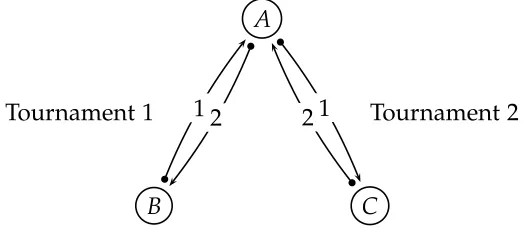
Let us clarify the setup. Let A,Band Cbe three subjects, and player 1 and player 2 be
two different roles in the tournament. Subject A plays one tournament (Tournament 1)
in player 2 role when he is matched with subject B who is in player 1 role, and another
one (Tournament 2) in player 1 role when he is matched with subjectsCwho is in player
2 role. Figure 4 depicts this scenario. All the treatments in our experiment are run
following this structure.
The basic structure of the games implemented in the experiments follows from
Sub-sections3.2.1and 3.2.2. Recall that player 1 and player 2 differ in two dimensions. First,
Figure4: Matching scheme in a typical round.
A
B C
2
1 21
Tournament 1 Tournament 2
2 is disadvantaged. Second, disadvantaged player can punish advantaged player in the
one-sided case (Subsection 3.2.1), while the opposite is not true. In the two-sided case
(Subsection3.2.2) however, both players can punish each other.
As we explained before (Figure 4), in each round of our experiment, each subject
is matched with two different subjects (opponents), therefore being involved in two independent tournaments: one where he is in the advantaged role and the other where he is in the disadvantaged role. Subjects are supposed to make their decisions for both
tournamentssimultaneously.
An experimental session lasts 34 rounds under different matching protocols, namely
fixed matching (f) and random matching (r). Under r subjects are randomly and
in-dependently matched at the beginning of each round, whereas under f subjects are
matched with other subjects and this match stays fixed.
In some treatments the first half (rounds 1-17) of the session is under f (r), while
second half (rounds 18-34) is under r(f). In other treatments the entire session (rounds
1-34) is either for r. In sum we have four matching schemes: fr, rf, ff, and rr, where,
for instance,frmeans rounds 1-17 arefand rounds 18-34 are r.
In treatments where matching scheme is fr or rf, when subjects enter the lab they
are told that the experiment is divided in two different parts, with the first one lasting for 17 rounds. Only when the first part is over do the subjects receive instructions for the second part of the session.
The final defining factor of our design concerns the information that the subjects are given between the tournament and punishment stages of the game. We have two
information regimes. In the low informationregime (l), after the subjects choose effort in
the tournament stage but before they make their punishment decision, they are given the information only about the effort choices of their opponents in the tournament. We also
have anhigh informationregime (h), where the subjects are given all the information about
[image:22.612.175.439.107.222.2]as the effort levels. This choice of design allows us to test our hypothesis cleanly since we can compare subjects’ responses to their opponent’s effort choices as well as their responses to outcomes that involve random factors beside effort choices.
Overall, we have four different treatments: 1-fr-ll, 1-rf-ll, 2-ff-lh, and 2-rr-lh. The
notation is self explanatory. For instance 2-ff-lhmeans that the treatment involves
two-sided punishment, the matching protocol is fixed in both halves of the session and, while in the first part of the experiment the subjects observed efforts before the punishment stage, in the second part of the experiment they observed the outcome payoffs of the tournament as well as the efforts.
We chose the tournament’s parameter values following SW. Particularly, subjects’
ef-fort levels were limited to the interval [0, 100] ( ¯e = 100.) We set α = 2 and we say that
a subject is in the disadvantaged role if the cost of effort is given by c(e) = αe2/150
(c = 150), otherwise we say that subject is in the advantaged role. The random shocks
that determine the outcome of the tournament lie in the range (−60, 60) (a = 60). The
prizes of the tournaments are M = 204 and m = 86. Additionally, we endowed each
player with D = 68 punishment points when they were in the disadvantaged role.
Ev-ery punishment point assigned to his opponent reduced his payoff by 3 punishment points. Every punishment point he kept was converted into US Dollars at the rate 1
point=$0.0015, while the exchange rate for each point earned in the tournament was
$1/322 points (h≈1.45 by exchange cross-rate.)
All the sessions were conducted at the Center for Experimental Social Science lab at New York University with a total of 68 participants, all students at that university.
The experiment was computerized using the software z-Tree (Fischbacher [13]). Sessions
lasted for about one hour and a half and participants received an average payment of
$24 dollars. All parameter values and procedures were common-knowledge. Table 1
presents our experimental design.
5
Results
In this section we will present our results by answering a set of questions generated by our theory.
5.1
Question 1: Do Subjects Punish when They Should
According to the Theory of Blame-Freeness?
Table1: Experimental design.
Treatment Matching Protocol Information Regime
1-fr-ll Fixed: rounds 1-17 Low: rounds 1-17
Random: rounds 18-34 Low: rounds 18-34
1-rf-ll Random: rounds 1-17 Low: rounds 1-17
Fixed: rounds 18-34 Low: rounds 18-34
2-ff-lh Fixed: rounds 1-17 Low: rounds 1-17
Fixed: rounds 18-34 High: rounds 18-34
2-rr-lh Random: rounds 1-17 Low: rounds 1-17
Random: rounds 18-34 High: rounds 18-34
we have stated before, while blame-freeness is a sufficient condition for no punishment, blameworthiness is only a necessary condition. Put differently, when a subject chooses more effort in the advantaged role than his advantaged opponent does against him while he is in the disadvantaged role, then our theory predicts unambiguously that we should see no punishment forthcoming. However, when a subject in the same position chooses less effort, then whether we see punishment occurring will depend on the cost of pun-ishment, its impact as a deterrent to the advantaged subjects, and the caring parameters of the subjects’ utility functions. If the cost of punishment is sufficiently high, the blame sufficiently small or the benefits sufficiently low in the eyes of the subjects, then we would not expect to observe any punishments.
In most of what we do below we will concentrate on the punishing behavior of the disadvantaged subjects. This makes more sense since strategically they are the ones for whom blame and punishment is most natural since they can blame their advantaged cohort for exploiting their advantaged position by choosing too high an effort level. In our one-sided punishment treatment, only the disadvantaged were allowed to punish so our focus on disadvantaged subjects is certainly natural there. While the advantaged subjects in our two-sided punishment treatment can also blame their disadvantaged cohorts by comparing what the disadvantaged subjects chose with what he would have chosen if he were disadvantaged, we think that comparison is less interesting. Still, at the end of this section we will investigate the punishing behavior of the advantaged subjects as well where indeed we will find some surprising results.
5.1.1 Punishment Levels: Disadvantaged Subjects
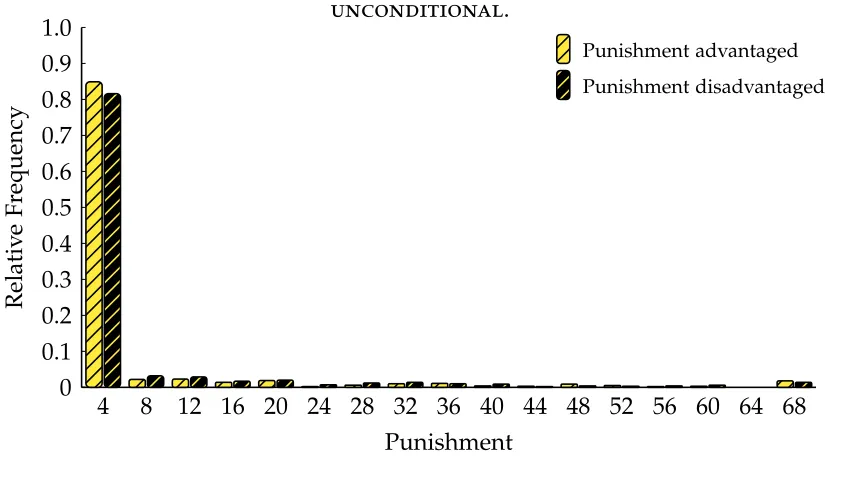
exper-iment in general. Figure 5 presents the average levels of punishment made by subjects in the disadvantaged role in both the one-sided and two-sided punishment treatments over their 34 rounds history. What is worth noting here is that mean punishment lev-els are clearly above zero so that punishment was an alternative employed by at least some disadvantaged subjects. Further, note that these are the punishments sent by the punisher and that the punishments received were three times this amount.
Figure 5: Average punishment in one-sided and two-sided treatments by the disadvantaged players.
0 1 2 3 4 5 6 7 8 9
0 3 6 9 12 15 18 21 24 27 30 33 36
b
b
b
b
b b b
b b b b b b b b b b b b b b b b b b b b
b b b
b b b b r r r r r r r r r r r r r r r r r r r r r r r r r r r r r r r r r r b One-sided treatments r Two-sided treatments Rounds A v er ag e P un is h m en t
5.1.2 Adherence to the Blame-Free Theory
[image:25.612.54.534.240.466.2]we actually observe no punishment in 983 cases.9 This clearly implies that subjects re-frained from punishing their advantaged opponents when those opponents acted in a more kind manner than they would if they were in their position.
Taking punishment behavior into account and not just non-punishing behavior, we see that of the subset of subjects who punished at least once, 73% of them exhibited behavior that did not violate the blame-free theory at least 50% of the time. This means they punished only when there was blame and failed to do so when there was none. More precisely, of the 68 subjects in our experiment 31 never punished, leaving 37 who did at least once. Such subsets of non-punishers are seen in almost all experiments where punishing exists since subjects are hesitant to punish their fellow subjects in almost all
laboratory experiments (see, for example, Fehr and Gaechter [11] where punishment
levels are quite low). In the end-of-session questionnaires distributed subjects report two main reasons for this behavior: the fact that punishment is costly and their unwill-ingness to hurt their opponents. Both of these reasons are consistent with our theory since the existence of blame is only a necessary condition for punishment and the cost of punishment is a reason not to do so. However, caring about one’s opponent means that
subjects have high caring parameters,bi’s, and hence it takes a lot of blame to force them
to punish. In fact, it is not clear how much punishment we should expect in our experi-ments since subjects with low caring parameters, self-centered individuals, are unlikely to blame their fellow competitors and therefore unlikely to punish them despite their
lowbiin their strategic preference function, while those with high caring parameters are
likely to blame their opponents but, since they care so much about them, unlikely to punish them. Hence, the level of punishment activity cannot easily be predicted but, as we have done, we can check for its theoretical consistency when it exists.
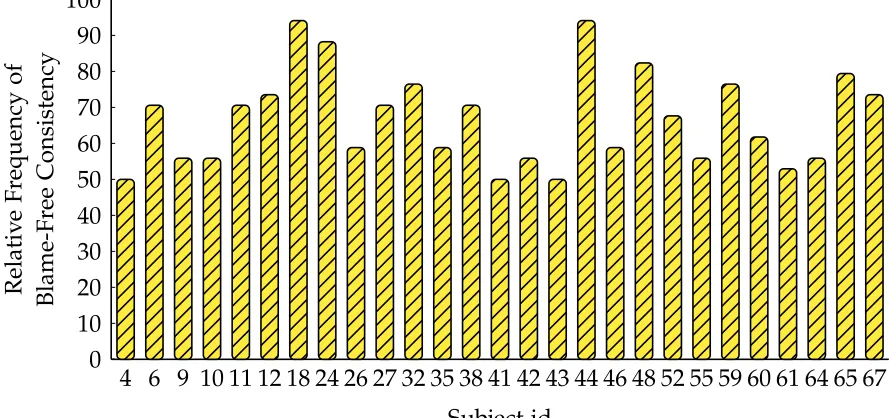
Figure6 indicates the consistency of subject behavior to our theory by that subset of
37 subjects who punished at least once and who were consistent with our theory at least 50% of the time.
Notice that the mean adherence is 68% with two subjects adhering as much as 94% of the time.
One cannot judge exactly whether this is strong or weak support for our theory be-cause not punishing blameworthy opponents may still be consistent with blame-freeness
as long as the caring parameter, bi, is high enough and the perceived costs are large
enough. Still, our data indicates that there is a non negligible part of the sample that
Figure6: Relative frequency of blame-free consistency for punishers who are consistent more than50% of the time: disadvantaged subjects.
0 10 20 30 40 50 60 70 80 90 100
4 6 9 10 11 12 18 24 26 27 32 35 38 41 42 43 44 46 48 52 55 59 60 61 64 65 67
Subject id
R
el
ati
v
e
F
re
q
ue
n
cy
o
f
B
la
m
e-F
re
e
C
o
n
si
ste
n
cy
haves according to blame-free principles when it comes to judge other person’s behavior. To get a better insight into whether disadvantaged subjects punished when they were supposed to according to the theory of blame-freeness, note that the observed behavior
of subjects would support it if subject jin the disadvantaged role punishes his opponent
subject i whenever j’s effort in the advantaged position is lower than i’s effort in that
same role. Of course these circumstances are only necessary conditions for punishment so requiring punishment when blame exists is a very strict test. Despite this fact, ceteris paribus, if our blame-free theory has teeth, it should be true that the probability of punishment is increasing in the amount of blame and that is a consequence we can
estimate. To do this we define the variable ∆ as difference between subject j’s effort
when he is advantaged and i’s effort when he is advantaged (while jis disadvantaged).
Since blame is decreasing in this difference, we would expect that the probability of
punishment would decrease with the variable ∆ and hence the coefficients associated
with this variable should be negative.
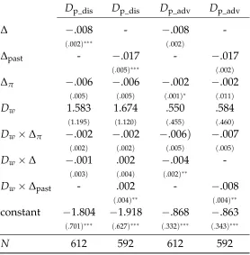
The first column in Table2shows the probit regression for the likelihood of punishing
in the disadvantaged role as a function of ∆. We denote the dummy variable that takes
value 1 when a disadvantaged subject punishes by Dp_dis. Note that the coefficient is
negative and significant, suggesting that the larger the deviation of i’s behavior with
respect to j’s behavior (the more negative the variable∆ is) the more likely jwill punish
i. In other words, asi’s behavior gets closer to j’s behavior (ini’s role), it is the less likely
[image:27.612.74.521.131.340.2]