SINTRACK ANALYSIS FOR TRACKING COMPONENTS
OF MUSICAL SIGNALS
PACS REFERENCE: 43.60.Gk
DAVID, Bertrand ; BADEAU, Roland ; RICHARD, Gaël
Ecole Nationale Supérieure des Télécommunications 46, rue Barrault
75634 Paris cedex 13 France
Tel: (33 1) 45 81 71 02 Fax: (33 1) 45 88 79 35 E-mail: [email protected]
ABSTRACT
Musical signals often present close frequencies producing beats and the classical Fourier Transform does not achieve a sufficient resolution to estimate these components separately with accuracy. This paper presents a spectral analysis technique for estimating and tracking the frequencies, damping factors and amplitudes of each component. SINTRACK associates a Matrix Pencil high resolution method with a LMS adaptive algorithm. It detects changes in the signal underlying model (as the changing number of sinusoids for example) and can indicate the time variations of parameters. Results are shown for a signal recorded from a guitar.
1 INTRODUCTION
A wide variety of musical sounds can be described schematically as a sum of harmonically related partials. However, the spectrum of a piano or a guitar is more complex. In some partials more than one elementary component is included whose close frequencies produce beats. These beats are known to be important features of the naturalness of a synthesized musical sound. They often result from the particular properties of vibrational systems: a minor lack of symmetry in a bell geometry leads to pairs of nondegenerate normal modes; the coupling between the strings and the bridge of a guitar is well described by a two dimensional mobility matrix, from which frequency doublets are derived [LAMBOURG93]; the multiple strings of a piano note are known to be slightly mistuned by excellent tuners in order to enhance the quality of the sound decay [WEINREICH77].
On the other hand, High Resolution techniques are complex and cannot be satisfactorily used for components tracking without modification. These methods are based on the assumption of a signal model whose parameters are taken constant with time. For example, they can not indicate the existence of a slow variation of the decay which could suggest a slight non linear behavior. Therefore, it is worthwhile to develop techniques allowing the tracking of the components at a lower complexity while keeping spectral resolution and accuracy. This constitutes the basic idea of SINTRACK. Our first attempt at applying SINTRACK to musical signals was made during the engineering school final work of M. Massabieaux [MASSABIEAUX00].
This paper first examines the principles of HR methods and the theoretical background of the SINTRACK algorithm. Then, simulation examples and a musical application will be presented.
2. THEORETICAL ASPECTS
SINTRACK [DUVAUT94] associates a HR technique (Matrix Pencil [HUA90]) to a low complexity adaptive algorithm (Least Mean Square or LMS). First, the Matrix-Pencil method is applied to obtain an initial estimation. Second, the components are tracked using the LMS procedure as long as the prediction error remains below a given threshold. When the error grows above the threshold, indicating that the model has become obsolete, Matrix-Pencil is applied again to reinitialize the frequency components estimates. Given that the complexity of the Matrix Pencil algorithm is O(N3) and that the complexity of LMS is O(N), the computational cost of SINTRACK is drastically reduced compared to Matrix Pencil alone if the components are well tracked. Also, it is important to note that SINTRACK can be used to detect model breaks (for example attacks) in a given signal. These breaks will correspond to frames where the LMS prediction error will abruptly grow.
2.1 High Resolution Principles
HR techniques rely on a precise signal model and are conventionally classified as parametric methods. This model represents the discrete signal
x
nas a sum of complex exponentials:∑ ∑ = = = − + = M i i i j i M i n i i
n b z A e j f n
x i 1 1 ] ) 2 exp[( ) ( φ α π
where
A
i,φ
if
iα
i respectively represent the initial amplitude, initial phase, frequency anddamping factor of each component. The estimation of (
f
i,α
i) is therefore a non linear problem. Prony [PRONY1795] first demonstrated that this signal can be predicted by means of a polynomial whose roots are the zi's. Finding the coefficients of this polynomial is a linearproblem. The estimation of
A
i,φ
ican be formulated as a linear least square problem if all other parameters are known.2.2 Matrix Pencil
We first define two backward data matrices
X
0andX
1using N samples of the signalx
nas follows:
=
− − − − − 2 1 2 1 1 0 N p N p NX
x
x
x
x
x
x
x
x
x
p 1 p 0L
M
M
M
M
L
L
;
=
− + − − + 1 1 1 3 2 2 1 1 N p N p NX
x
x
x
x
x
x
x
x
x
p pL
M
M
M
M
L
L
Matrix Pencil rely on the rank reducing property of the zi's for the pencil of matrices
X
1−
zX
0.+
1
X
denotes the order M truncated pseudo-inverse of the rank-M matrixX
1.X
1+ is obtained using the Singular Value Decomposition (SVD) which is expressed as:H
V
U
X
1=
∑
where the subscript H denotes the conjugate transpose and where
∑
has M non-zeros elements on the diagonal, sorted in decreasing order. LetU
M andV
M be the matrices builtwith the M first columns of
U
andV
respectively.X
1+is obtained by inverting the M non-zeros singular values in∑
. This can be written:H M
M
U
V
X
1+=
∑
+It should be noticed that when a white noise is added to the model, the matrix X1 becomes
full-rank, all of its singular values being increased by the variance of the noise. Its M principal right and left eigenvectors remain unchanged. The Matrix Pencil method is then applied without any further modification. The M selected vectors in matrices
U
M andV
M correspond to the Mlargest singular values, denoted as
λ
i, i = 1...M. The values of the frequencies and damping factors are then derived asf
i=
−
arg(
λ
i)
/(
2
π
)
andα
i=
ln
λ
i2.3 LMS For Tracking The Poles
The adaptive Least Mean Square algorithm is used to track the poles of the signal once they have been estimated with matrix pencil. The prediction coefficients in the backward direction are given in the vector bn and thus provide an estimation of xn as a linear combination of his future:
n n T n
n
e
x
=
b
x
+1+
, where xn+1=[xn+1 xn+2 ... xn+p] Tand en is the prediction error. At initial time n=0,
this vector is given by
V
MU
MH[
x
0x
1x
N−p−1]
T+
∑
−
=
L
0
b
and updated following the well-knownrelation
b
n=
b
n−1−
µ
e
n−1x
n where µ is the adaptation step of the LMS. The poles of the signal are derived as the roots inverses of the polynomial p(z) = zp+ [zp-1 zp-2 ... 1]bn.2.4 Algorithm And Practical Choices
The SINTRACK algorithm can be separated in 2 steps:
1 initialization: matrix pencil is applied to find the initial values of the zi's and b0
2 tracking:
• the roots of p(z) are extracted in order to estimate the updated poles,
• the corresponding complex amplitudes ( j i
i
e
A
φ ) are estimated by minimizing the quadratic error between the real data and the estimates over the range of the p future observations,• the prediction error is evaluated: if e(n) is above the threshold then the initialization step is rerun, else the tracking continues for the following frame.
We now address the problem of parameter tuning for Matrix Pencil and the LMS.
The number M of components is generally unknown. The results of the estimation are much affected if M is underestimated. A usual choice is to overestimate the value of M. The true value can be approached further regarding the fact that real poles lay outside the unit circle, when the others fall inside.
The adaptation step µ of the LMS must be chosen and updated to be less than 2/(pEn 2
) where
∑
−= +
−
=
10 2 1
1 2
p
k k n p
n
x
E
This insures the convergence of the algorithm while taking into account the intrinsic non stationarity of the signal energy.
At last, the threshold can be chosen following two ways. Either an estimate of the noise variance σ2 is known and we can state it as 3σ for example, or we can consider that the initialization step must occur when the prediction error is above a fraction of the maximal amplitude (typically situated between 1/10 and ½)
3. SIMULATIONS AND APPLICATION TO A PIANO PARTIAL
3.1 Tracking Of A Single Component With Double Decay
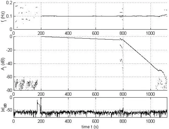
This example aims at demonstrate the decay tracking capability of the algorithm. The synthetic signal is made of a single component whose frequency is 0.1 samples-1 and a unitary initial amplitude (A=1). Its decay takes the values 0.001 and 0.02, one after the other. The onset of the component stands on discrete time n=200 and a white gaussian complex noise of 0.001 standard deviation is added, which corresponds to an overall SNR of approximately 55dB. This resembles to the Decay-Release envelope of a musical sound.
The Figure 1 shows the results of the tracking for the frequencies fi and the amplitude Ai, for
analysis parameters N=80, M = 6 and a 3σ threshold. The figure does not show the estimation of the αi’s whose accuracy is very poor, considering the small value of N. However, they can be
derived from the Ai’s tracking by a simple linear regression. The figure clearly shows the sudden
[image:4.596.156.434.460.673.2]growths of the prediction error at the onset-time and at the decay changing time. We can notice that the prediction error remains high in the regions before n=200 and n=800, where model jumps occur in the analysis window.
Figure 1: a single component with double decay
3.2 Detection Of The Onsets Of Delayed Damped Sinusoids
1 and a second one beginning at n=400, ending at n=800 with parameters f=0.12, α=0.004, A = 1. The additive noise has a standard deviation σ=0.001 (approximately 55dB SNR). The analysis parameters remain unchanged from the previous example. The results shown on figure 2 demonstrate both the accuracy of the estimation and the precision for detecting model jumps.
Figure 2: detection of the onset and the extinction of a sinusoid in presence of an other one
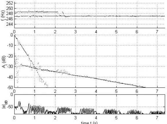
3.2 Application To A Guitar Partial
For this application, the E2 note of a classical guitar was recorded and sampled at 48kHz. A piezoelectric crystal was specially designed for that purpose and integrated in the saddle. As a result, the measured signal is proportional to the transverse force applied by the string to the bridge. A preprocessing step was needed both to enhance the resolution and to shorten the data. The signal was first filtered with a FIR Remez Filter, designed to isolate the 3rd harmonic (partial at 247.5Hz). The filtered signal was then demodulated and downsampled by a factor 384. The preprocessed signal was complex and 1700 samples long (7 seconds). The results are displayed using Hz and seconds for convenience. The analysis parameters were N=80 (0.64s), M = 6 and the threshold was taken as 1/10 of the maximum amplitude.
[image:5.596.150.438.520.735.2]The results displayed on figure 3 clearly show two principal components, one with a high initial amplitude and short decay while the other has a much lower amplitude with a longer decay. This is consistent with the known properties of free vibrating strings coupled to a bridge: the horizontal and vertical polarizations of the vibration are coupled by the bridge which leads to frequency doublets. The vertical polarization excites transverse motions of the plate and thus corresponds to high initial level and shorter decay [JANSSON83].
These results demonstrate the validity of a complex exponential model for the components of a guitar tone. It also allows an accurate estimation of the parameters of these components. However, some drawbacks should be mentioned. As the saw-tooth behavior of the prediction error suggests, the threshold is often reached. Matrix pencil is therefor frequently applied which yields to a greater complexity. To reduce this phenomenon the adaptation step µ could be diminished but at the cost of a less efficient tracking since the convergence of the LMS is slower.
4. CONCLUSION AND FUTURE WORKS
SINTRACK is an efficient method to study and accurately estimate the musical signals whose spectrum is composed with possibly varying close frequency components. By associating a High resolution method with a tracking approach, SINTRACK has the potential to accurately locate abrupt changes in the signal content and therefore should represent a useful tool for signal onset (or transients) detection.
Future works include the study of the attack of musical tones and the estimation of the piano decays.
References
[BOYER02] Boyer R., Essid S.and Moreau N. (2002). Non-stationary signal parametric modeling techniques with an application to low bitrate audio coding. IEEE International Conference on Signal Processing, August 2002.
[DAVID99] David, B (1999). Caractérisation acoustiques de structures vibrantes par mise en atmosphère raréfiée. Phd Thesis, University of Paris VI.
[DUVAUT94] Duvaut, P. (1994). Traitement du signal, Chap. 11, Hermes ed.
[HUA90] Hua, Y and Sarkar T.K. (1990). Matrix pencil method for estimating parameters of exponentially damped/undamped sinusoids in noise. IEEE Trans. Acoust., Speech, Signal Processing ASSP-38, 814-824.
[JANSSON83] Jansson, E. V. (1983). Acoustics for the guitar player. In “Function, construction and quality of the guitar” (E.V. Jansson ed.). Stockholm. Royal Swedish Academy of Music.
[JEANNEAU98] Jeanneau, M., Mouyon P. and Pendaries C. (1998). Sintrack analysis, application to detection and estimation of flutter for flexible structures. EUSIPCO 98, pp 789-792.
[LAMBOURG93] Lambourg, C and Chaigne, A. (1993). Measurements and modeling of the admittance matrix at bridge in guitars. In SMAC, Stockholm. Royal Swedish Academy of Music.
[LAROCHE93] Laroche, J. (1993). The Use of the matrix pencil method for the spectrum analysis of musical signals. Journal of the Acoustical Society of America 94(4), 1958-65. [MASSABIEAUX00] Massabieaux, M (2000). Estimation and tracking of the components of a
musical signal (in french). Ecole Nationale Supérieure de l’Electronique et de ses Application. Report of the engineering school final work. Unpublished.
[PRONY1795] Prony, R. (1795). Essai expérimental et analytique. Anales de l’Ecole Polytechnique 1(2).