Active Routing in Ad Hoc Networks Edición Única

Texto completo

(1)Instituto Tecnológico y de Estudios Superiores de Monterrey Campus Monterrey División de Electrónica, Computación, Información, y Comunicaciones Programa de Graduados. Active Routing in Ad-Hoc Networks THESIS Presented as a partial fulfillment of the requeriments for the degree of Master of Science in Electronic Engineering Major in Telecommunications. Ing. Alejandro Rivera Leal Monterrey, N.L. May 2007.

(2) c Alejandro Rivera Leal, 2007 °.

(3) Instituto Tecnológico y de Estudios Superiores de Monterrey Campus Monterrey División de Electrónica, Computación, Información, y Comunicaciones Programa de Graduados. The members of the thesis committee recommended the acceptance of the thesis of Alejandro Rivera Leal as a partial fulfillment of the requeriments for the degree of Master of Science in: Electronic Engineering Major in Telecommunications THESIS COMMITTEE. Cesar Vargas Rosales, Ph.D. Advisor. Jose Ramón Rodriguez Cruz , Ph.D.. Artemio Aguilar Coutiño, M.Sc. Synodal. Synodal. Approved Graciano Dieck Assad, Ph.D. Director of the Graduate Program. May 2007.

(4) Gracias a Dios por darme la oportunidad de realizar mis estudios de postgrado, y el porque me da la oportunidad de seguir mi camino junto con mi familia, mi novia y mis amigos. Mi trabajo de Tésis esta dedicado a: Mis padres, Alejandro C. y Ma. de la Luz, A mis hermanos Paola y César, A mi novia y prometida Margot, A mi tı́a, Blanca Alicia, Les doy gracias por estar siempre conmigo, Les quiero mucho y los amo..

(5) Acknowledgments My personal thanks to my advisor Ph.D. César Vargas Rosales for their teaching, advises, friendship, thanks for the great interest in the realization of this work. I want to thank the member of my thesis committee Artemio Aguilar Coutiño, M.Sc. and Jose Ramón Rodriguez Cruz, Ph.D. for their valuable comments and advises in my thesis work. Thanks to my friends, Armando, Carolina, Eduardo, Emeterio, Javier, Jonam, Jose Angel, Jose B., Jose Luis, Lucero, Raul, Ricardo G. and Rosa Marı́a, thanks for your the real friendship. And Servando, thanks for give advices, opinions and for your interest in this thesis work, your experience in your thesis of Solitons help me a lot for the realization of my work.. Alejandro Rivera Leal Instituto Tecnológico y de Estudios Superiores de Monterrey May 2007.

(6) Active Routing in Ad-Hoc Networks. Alejandro Rivera Leal, M.Sc. Instituto Tecnológico y de Estudios Superiores de Monterrey, 2007. Abstract The great interest in wireless networks has been tested recently offering a set of different possibilities for mobile users, that are bringing us closer to voice and data communications “anytime and anywhere”. Some outstanding solutions in this field are Wireless Local Area Networks, that offer high-speed data rate in small areas, and Wireless Wide Area Networks, that allow a greater mobility for users. In different cases, just like the rescue operations, emergency and military environments, the need to establish a dynamic communications with no reliance on any kind of infrastructure is very important. Then, the easy of fast deployment that ad hoc networks provides us becomes of great usefulness. Ad hoc networks are integrated by mobile hosts that work together with each other in a distributed way for the transmissions of packets over wireless links, their routing, and the management of the network itself. Their features condition their design in several network layers, so that parameters like bandwidth or energy consumption, that appear critical in a multi-layer design, must be carefully taken into account. This work, is made with the intention to find questions and research problems, is very important for the design of an ad hoc network to study some of their critical design and performance issues. As the throughput per node is identified as the limiting factor in their performance, the bounds that available network capacity can achieve are considered, as well as the different factors that impact on this capacity and, consequently, that suggest possibilities to increase it. Furthermore, the problems routing algorithms for ad hoc networks have to solve are investigated, in addition to the medium access control mechanisms. There exists a significant dependence between the medium access control layer and the network layer, and, indeed, a complete integration of the diverse design solutions available.

(7) in the different network layers of the protocol stack is still not achieved. This thesis also includes a review about quality of service mechanisms in ad hoc networks..

(8) Active Routing in Ad-Hoc Networks. Alejandro Rivera Leal, M.Sc. Instituto Tecnológico y de Estudios Superiores de Monterrey, 2007. Resumen El rápido crecimiento que han tenido las redes inálambricas en los ultimos años, ha proporcionado a los usuarios diferentes alternativas que ayudan a que la comunicacion sea lograda desde cualquier lugar y en diferente momento. Las opciones mas conocidas en el campo de redes inálambricas estan las de área local (WLAN´s) que ayudan a la transmisión de datos a mayor velocidad y también estan las redes inálambricas de área extendida (WWAN´s) donde los usuarios de la red tienen una mayor movilidad. En otras situaciones, como las operaciones de emergencia o como aplicaciones de uso militar, se necesita establecer una comunicación mas dinámica, osease que no se requiere ningun tipo de infraestrutura de tipo alámbrica. Es por eso, que las redes inálambricas de comunicación “ad hoc” resultan y suelen tener mucha utilidad. Las redes ad hoc están formadas por dispositivos móviles que trabajan de manera conjunta con la finalidad de llevar a cabo la transmisión de los paquetes por los enlaces inalámbricos que forman la red, el encamiento de dichos paquetes y la gestión y el mantenimiento de la red misma. Sus peculiares caracterı́sticas y limitaciones condicionan sobremanera el diseño en varios de los niveles OSI de red, de forma que parámetros como el ancho de banda o el consumo energético, que tienden a ser crı́ticos en un diseño multinivel como el que parece apropiado para las redes ad hoc, deben ser tomados en cuenta de manera especialmente cuidadosa. El trabajo de Tesis esta realizado con el objetivo de identificar cuestiones abiertas y problemas de investigación en este campo, es un estudio acerca de las redes ad hoc que se centra en temas crı́ticos relativos a su eficiencia y diseño..

(9) Contents. List of Figures. iii. List of Tables. v. Chapter 1 Introduction 1.1 Objective . . . . . . . . . . . . . . . . . . . . . . . . . . . . . . . . . . . . 1.2 Justification . . . . . . . . . . . . . . . . . . . . . . . . . . . . . . . . . . . 1.3 Organization of the Thesis . . . . . . . . . . . . . . . . . . . . . . . . . . .. 1 2 2 3. Chapter 2 Background 2.1 Wireless Networks. . . . . . . . . . . . . . . . . . 2.2 Wireless Ad Hoc Networks . . . . . . . . . . . . . 2.3 QoS in Ad-Hoc Networks . . . . . . . . . . . . . . 2.3.1 QoS Models . . . . . . . . . . . . . . . . . 2.3.2 Special Issues and Difficulties in MANETS 2.3.3 Disadvantage of the Different QoS Models 2.4 Classification of Routing in Ad-Hoc Networks . . 2.4.1 Proactive Routing Protocol . . . . . . . . 2.4.2 Reactive Routing Protocol . . . . . . . . . 2.4.3 Hybrid Routing Protocol . . . . . . . . . . 2.5 Active Routing . . . . . . . . . . . . . . . . . . . 2.5.1 Advantages of Active Routing . . . . . . . 2.5.2 Active QoS Routing (AQR) . . . . . . . . 2.5.3 Active Routing in Ad Hoc Networks . . . 2.5.4 Conventional Routing vs Active Routing . 2.5.5 Route Discovery and Route Maintenance .. . . . . . . . . . . . . . . . .. 5 5 8 10 11 11 12 13 13 15 17 19 19 20 20 21 23. Chapter 3 Proposed Model 3.1 Mobility Model . . . . . . . . . . . . . . . . . . . . . . . . . . . . . . . . . 3.2 Beacon Packets . . . . . . . . . . . . . . . . . . . . . . . . . . . . . . . . .. 25 27 27. i. . . . . . . . . . . . . . . . .. . . . . . . . . . . . . . . . .. . . . . . . . . . . . . . . . .. . . . . . . . . . . . . . . . .. . . . . . . . . . . . . . . . .. . . . . . . . . . . . . . . . .. . . . . . . . . . . . . . . . .. . . . . . . . . . . . . . . . .. . . . . . . . . . . . . . . . .. . . . . . . . . . . . . . . . .. . . . . . . . . . . . . . . . .. . . . . . . . . . . . . . . . .. . . . . . . . . . . . . . . . ..

(10) ii. CONTENTS 3.3. . . . . . .. 28 28 30 30 32 33. . . . .. 37 37 38 41 42. Chapter 5 Conclusions and Further Research 5.1 Conclusions . . . . . . . . . . . . . . . . . . . . . . . . . . . . . . . . . . . 5.2 Future Research . . . . . . . . . . . . . . . . . . . . . . . . . . . . . . . . .. 49 49 50. Bibliography. 51. Vita. 53. 3.4. 3.5. Shortest Path Routing . . . . . . . . . . . . 3.3.1 Dijkstra Algorithm . . . . . . . . . . Active Routing Algorithm . . . . . . . . . . 3.4.1 Shortest path routing Diagram . . . 3.4.2 Multi-path Diagram . . . . . . . . . Effects of the Physical Layer in our model of. Chapter 4 Numerical Results 4.1 Proposed scenarios . . . . 4.1.1 Scenario 1 . . . . . 4.1.2 Scenario 2 . . . . . 4.1.3 Scenario 3 . . . . .. . . . .. . . . .. . . . .. . . . .. . . . .. . . . .. . . . .. . . . .. . . . .. . . . .. . . . . . . . . . . . . . . . . . . . . . . . . . . . . . . . . . . . . . . . . . . . . . Active Routing. . . . .. . . . .. . . . .. . . . .. . . . .. . . . .. . . . .. . . . .. . . . .. . . . . . .. . . . .. . . . . . .. . . . .. . . . . . .. . . . .. . . . . . .. . . . .. . . . . . .. . . . .. . . . . . .. . . . .. . . . . . .. . . . ..

(11) List of Figures. 2.1 2.2 2.3 2.4 2.5 2.6 2.7 2.8. Different kind of wireless networks . Wireless LAN Example . . . . . . . Wireless Cellular Example . . . . . Wireless Ad Hoc Example . . . . . Ad Hoc Routing Protocols . . . . . Network Using ZRP . . . . . . . . Example of conventional routing . Example of active routing . . . . .. . . . . . . . .. . . . . . . . .. . . . . . . . .. . . . . . . . .. . . . . . . . .. . . . . . . . .. . . . . . . . .. . . . . . . . .. . . . . . . . .. . . . . . . . .. . . . . . . . .. 6 7 7 8 14 18 22 22. 3.1 3.2 3.3 3.4 3.5 3.6 3.7 3.8 3.9 3.10. Network with 10 nodes . . . . . . . . . . . . . . . . . . . Network Using ZRP protocol . . . . . . . . . . . . . . . . Network with mobility . . . . . . . . . . . . . . . . . . . . An example with a simple Dijkstra . . . . . . . . . . . . . Example solved with Dijkstra algorithm . . . . . . . . . . Block diagram of shortest path routing . . . . . . . . . . . Block diagram of multi-path . . . . . . . . . . . . . . . . Example of one multi-path with one and two ramifications Example of 1 multi-path with one ramification . . . . . . Example of 1 multi-path with 2 ramifications . . . . . . .. . . . . . . . . . .. . . . . . . . . . .. . . . . . . . . . .. . . . . . . . . . .. . . . . . . . . . .. . . . . . . . . . .. . . . . . . . . . .. . . . . . . . . . .. . . . . . . . . . .. 26 26 28 29 30 31 33 34 34 34. 4.1 4.2 4.3 4.4 4.5 4.6 4.7 4.8 4.9 4.10. Packet loss ratio with no mobility and λ = 7 . . . . Packet loss ratio with no mobility and λ = 10 . . . Carried traffic with no mobility and λ = 7 . . . . . Carried traffic, no mobility and λ = 10 . . . . . . . Packet loss ratio with medium mobility and λ = 7 Packet loss ratio with medium mobility and λ = 10 Carried traffic with medium mobility and λ = 7 . . Carried traffic, medium mobility with λ = 10 . . . Packet loss ratio with high mobility and λ = 7 . . Packet loss ratio with high mobility and λ = 10 . .. . . . . . . . . . .. . . . . . . . . . .. . . . . . . . . . .. . . . . . . . . . .. . . . . . . . . . .. . . . . . . . . . .. . . . . . . . . . .. . . . . . . . . . .. . . . . . . . . . .. 39 39 40 40 42 43 43 44 45 45. iii. . . . . . . . .. . . . . . . . .. . . . . . . . .. . . . . . . . .. . . . . . . . .. . . . . . . . .. . . . . . . . .. . . . . . . . .. . . . . . . . .. . . . . . . . . . .. . . . . . . . .. . . . . . . . . . .. . . . . . . . .. . . . . . . . . . .. . . . . . . . . . ..

(12) iv. LIST OF FIGURES 4.11 Carried traffic with high mobility, with λ = 7 . . . . . . . . . . . . . . . . 4.12 Carried traffic, high mobility and λ = 10 . . . . . . . . . . . . . . . . . . .. 46 47.

(13) List of Tables. 4.1 4.2 4.3 4.4 4.5 4.6 4.7. Parameters for ZRP implementation with zero mobility . . . . . . . . Improvement of Packet Loss Ratio with no mobility and λ = 7 . . . . Improvement of Carried traffic with no mobility and λ = 7 . . . . . . Improvement of Packet Loss Ratio with medium mobility and λ = 10 Improvement of Carried traffic with medium mobility and λ = 10 . . Improvement of Packet Loss Ratio with high mobility and λ = 7 . . . Improvement of Carried traffic with high mobility and λ = 7 . . . . .. v. . . . . . . .. . . . . . . .. . . . . . . .. 38 41 41 42 44 46 46.

(14) vi. LIST OF TABLES.

(15) Chapter 1 Introduction. Wireless networks are becoming increasingly popular, and are more widely used than wired networks. With the onslaught of personal digital assistants (PDAs) and tablets, and access to calendars, e-mail, addresses, phone numbers and even the Internet, connectivity is becoming a “way of life”. The circumstances of these communications can vary tremendously depending on the context, and the traditional infrastructure networks are not functional in some occasions, for instance, when the network has to be established quickly or when the terrain becomes inhospitable. Therefore, the demand of easily deployable infrastructureless networks is utterly justified. Such networks are called ad hoc networks (AHNs) and they possess the important characteristic of having decentralized topology, so that the devices do not need the use of any kind of fixed network element for the communication between them, but they administrate the network resources in a distributed way. With this decentralized architecture, they should be able to adapt themselves to changes in the number of the nodes, their location and the traffic pattern requirements. Furthermore, the mobility of the nodes is another relevant point to allow communication of endpoints, which may be moving as well and are unaware of any other mobility pattern in the network. The wireless nature of the links used in ad hoc networks and the fact that the nodes employ a part of their resources (bandwidth, power, etc.) to send other nodes packets, limits the throughput available for each node. When the number of nodes becomes high, scalability problems appear and this issue turns out to be critical. Therefore, capacity should be managed properly and the parameters affecting it, should be designed carefully. All these attributes that define the behavior of this kind of networks have important 1.

(16) 2. CHAPTER 1. INTRODUCTION. implications in their engineering, affecting to several network layers. Obviously, the form of routing, for instance, is especially specific, since two nodes that may establish an information exchange might not be able to communicate directly, so the routing scheme becomes multihop and the cooperation between stations turns out to be fundamental in order to manage mobility and to deliver packets. Therefore, in this environment, the hosts need to behave also as routers, because they should forward the packets they receive from their neighbors by following a particular routing algorithm. Ad-hoc wireless networks are self-organized, and self-managed, [1]. An Ad-hoc network starts with 2 nodes transmitting their presence (making beacons) with their respective address information.. 1.1. Objective. The purpose of this work is to identify and to implement an efficient Ad Hoc wireless network and modify it using an active routing protocol. This evaluation should be done through simulation. To implement an active routing protocol, we decide that the nodes of the network take important decisions when any emergency situation in our scenario happens, for example, a broken link or a blocked node by too much traffic.. 1.2. Justification. The idea of a communication system is to create an excellent topology and facilitate service to the users when they require to use it, accordingly the service requires to be fast, efficient and with an excellent Quality of Service (QoS). Wireless networks propose solutions and services summing up high mobility. They make indispensable the growth of new and better algorithms for routing protocols. QoS for Ad hoc networks is a new area of research, so the concepts to be appreciated are connectivity, security, mobility, interference, offered network load, network size, carried traffic, packet loss ratio, average end-to-end delay, etc..

(17) 1.3. ORGANIZATION OF THE THESIS. 3. This thesis deals with some important issues concerning ad hoc networks, natural inheritors of packet radio networks.. 1.3. Organization of the Thesis. The organization of this thesis is the following one: In Chapter 2, the general concepts of wireless networks and wireless Ad-Hoc networks as well as different topics like Quality of Service (QoS) in ad hoc networks and concepts concerning routing in ad hoc networks. In Chapter 3 presents and describe a model proposed for the thesis. In Chapter 4 we presents the results using the model developed in Chapter 3, and the evaluation of the simulations. In Chapter 5 contains the conclusions of the thesis with the future work..

(18) 4. CHAPTER 1. INTRODUCTION.

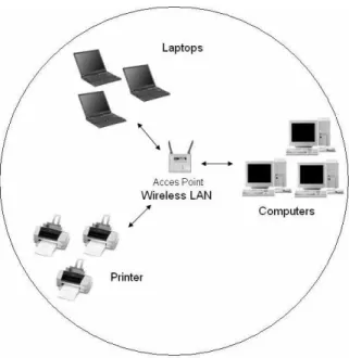
(19) Chapter 2 Background The next sections present the main concepts that are useful for the thesis, an explanation of wireless networks, ad hoc networks, also the different routing protocols in the ad-hoc network (MANET), and concepts of quality of service in ad hoc networks.. 2.1. Wireless Networks.. Today’s evolution of wireless networks is one of the most dynamic developments in both, telecommunication and data communication. Technological improvements enable new services like cellular networks, LAN’s and Mobile Ad Hoc networks (MANET) be a solution where a wire-line could be a problem in a specific net, [2]. These kind of networks are shown in Figure 2.1, where we can see the Ad Hoc network as part of the infrastructureless networks. Several wireless interface standards for WLAN currently exist, some operate within licensed and others within unlicensed spectrum, some point to point, others point to multipoint, and yet others more flexible. The most common readily available standard at the moment is the 802.11 family (802.11, 802.11a, 802.11b and 802.11g). This is consumer equipment that operates on an unlicensed radio frequency. Each wireless network is composed of various nodes connected together. A node is a collection of various PCs or other equipment connected together directly using the IP network and within direct radio range. A node consists of at least one router and one or more clients. The clients normally require little configuration and talk only to the router, whilst the router will route its own data and that of its clients to the rest of the network. It will also participate in exchange routing information with other nodes to ensure it always knows how to reach the rest of the network. The nodes can be connected together by radio links or by other means. The term node can loosely be associated with the router/host which manages each node within 5.

(20) 6. CHAPTER 2. BACKGROUND. Figure 2.1: Different kind of wireless networks. its own local network. Due to the limited range of the radio signals a large number of nodes will be required to provide coverage to a whole town, thus requiring a complex mesh of connections between the nodes to provide a robust network. The network clients, the people who connect to the nodes from their home or office, make up the complete network. The nodes without clients form the network infrastructure. Figure 2.2, shows an example where a LAN network is set up using a small base stations (access point) that manage the traffic flows that users generate in its coverage area. Also the base station acts like a gateway, in order to connect with other base stations and communicate nodes in different network cell. The Personal communication Network (PCN) concept enable people to call other people, not just places or terminals. The name/adress of a network point of attachment will no longer identify a terminal at call setup. The PCN will allow a subscriber to establish and receive calls across different networks at any user-network interface mobile, [2]. The geographic area covered in a wireless PCN is partitioned into cells, each of which has a base station. To accommodate the predicted growth in mobile subscribers, cell dimensions should be reduced from the size currently used in mobile radio systems. Figure 2.3, shows a cellular network providing a service to cellular users. This kind of.

(21) 2.1. WIRELESS NETWORKS.. 7. Figure 2.2: Wireless LAN Example. network needs investments in base station infrastructure per network cell that will manage the traffic generated by all users inside its coverage area.. Figure 2.3: Wireless Cellular Example. Ad hoc wireless networks consist of mobile nodes interconnected by multihop communication paths. Unlike conventional wireless networks, ad hoc networks have no fixed network infrastructure or administrative support. The topology of the network changes dynamically as mobile nodes join or depart the network or radio links between nodes become.

(22) 8. CHAPTER 2. BACKGROUND. unusable. This is a complex and difficult issue because of the dynamic nature of the network topology and generally imprecise network state information. In addition, people also recognize that ad hoc networking has obvious potential application in all the traditional areas of interest for mobile computing. Numerous challenges must be overcome to realize the practical benefits of ad hoc networking, [1]. In Figure 2.4, a group of mobile nodes are disperse on a two dimensional plane. The information of the origin, needs to travel across the different nodes to arrive in a previously defined destination.. Figure 2.4: Wireless Ad Hoc Example. 2.2. Wireless Ad Hoc Networks. In a future, telecommunication technology will be principally founded on wireless technology. Wireless is completely multidimensional, and wireless mobile and access will come together to be more like ad hoc characteristics. Ad hoc technology will be one of primary points in the wireless communications, large area mobile multihop wireless and personal access networks, [3]..

(23) 2.2. WIRELESS AD HOC NETWORKS. 9. A mobile ad hoc network (MANET) is a group of mobile, wireless nodes which cooperatively and spontaneously form an IP-based network. This network is independent of any fixed infrastructure or centralized administration. A node communicates directly with nodes within its wireless communication range. Nodes that are part of the MANET, but beyond each other wireless range, communicate using a multi-hop route through other nodes in the network. These multi-hop routes change with the network topology and are determined using a routing protocol. Wireless Ad Hoc networks have some problems which should be considered in a routing protocol design with the objective to compare the different route options. Those problems are listed below, [4],. 1. Scalability: Ad/Hoc networks do not allow the same kinds of aggregation techniques so they are vulnerable to scalability. Node mobility also introduce other kind of scalability problems 2. Protocol Deployment and Incompatible Standards: Wireless ad/hoc network protocol is susceptible to forces working versus standardization 3. Wireless Data Rates: This problem is because the adoption of wireless computing. It is clear the difference in speed of wired and wireless networks 4. Security: traffic across an ad hoc network can be highly vulnerable to security problems. Thus, existing techniques for securing network protocol transactions for wired networks must also be applied to the techniques of ad hoc networks. 5. Spotty Coverage: The coverage gaps make it unlikely that people in affected regions will invest in most existing wireless devices because of the dependency on infrastructure support for their operation. In mobile ad-hoc networks, topology is highly dynamic and random. In addition, the distribution of nodes, and, eventually, their capability of self-organising play an important role. The main characteristics can be summarized as follows: 1. The topology is highly dynamic and frequent changes in the topology may be hard to predict. 2. Mobile ad-hoc networks are based on wireless links, which will continue to have a significantly lower capacity than their wired counterparts..

(24) 10. CHAPTER 2. BACKGROUND 3. Physical security is limited due to the wireless transmission. 4. Mobile ad-hoc networks are affected by higher loss rates, and can present higher delays and jitter than fixed networks due to the wireless transmission. 5. Mobile ad-hoc network nodes rely on batteries or other exhaustible means for their energy. As a consequence, energy savings are an important system design criterion. Furthermore, nodes have to be power-aware: the set of functions offered by a node depends on its available power (CPU, memory, etc..).. 2.3. QoS in Ad-Hoc Networks. QoS in ad hoc networks is a recently researched topic. The evolution of effective and appropriate protocols to substantiate the different networking performances in a mobile ad hoc network demonstrates a lot of issues to the fact that such networks have rapidly changing, random, multihop topologies, [5].Some issues, are mentioned below:. • Routing information accuracy, In a wireless Ad Hoc network, the available state information for routing includes inaccuracies due mainly to user mobility, increasing and variable delays or even lost of control packets. Routing protocols should attempt to reduce the impact of those inaccuracies on the efficiency and reliability of their operation. • Power Consumption, An important factor is the limited power supply, which can inhabit packet forwarding in an Ad Hoc network. There are two methods to optimizing the power consumption, the first one is to minimized the average power dissipated by the individual nodes and the second one is to minimized the overall power dissipated trough out the network on the average under the technique adopted. • Reliability, This issue is very important in some applications, offering reliable delivery of data to a group of fast moving nodes that change their position continuously add complexity to the problem of efficient communication on the net • Interoperability Adaptability, Some of the solutions in ad hoc networks doesn’t apply from those offered in fixed networks. However host should be able to travel free across Ad Hoc network, fixed infrastructure wireless and wired networks. • Security, Since communication traffic may pass trough unprotected links or routers and since there are some applications who in many cases are of high security, for.

(25) 2.3. QOS IN AD-HOC NETWORKS. 11. example: military cases, so the effort to control the security in a network is increasing continuously to provided a secure communication This section discusses unique issues and difficulties for supporting QoS in a MANET environment and ends up showing the major drawbacks of each of the two QoS architectures described above with respect to these characteristics.. 2.3.1. QoS Models. QoS is a term widely used in the last recent years in the area of wire-based networks. QoS stands for Quality of Services and the truth is that there is much debate on what exactly QoS is supposes to mean. Most vendors implement QoS protocols having in mind specific scenarios and taking into consideration different parameters, network topologies and variables. Todays Internet applies best effort IP forwarding. The network attempts to deliver all traffic as soon as possible within the limits of its abilities, but without guarantees related to throughput, delay or packet loss. It is left up to the end systems to cope with network transport impairments. Although best effort will remain adequate for most applications, QoS support is required to satisfy the growing need for multimedia over IP, like video streaming or IP telephony. The existing QoS models can be classified into two types according to their fundamental operation; the Integrated Services framework provides explicit reservations end-to-end and the Differentiated Services architecture offers hop-by-hop differentiated treatment of packets.. 2.3.2. Special Issues and Difficulties in MANETS. MANETs differ from the traditional wired Internet infrastructures. The differences introduce difficulties for achieving Quality of Service in such networks, [5]. The following list itemizes some of the problems: • Dynamic Topologies: nodes are free to move arbitrarily; thus, the network topology which is typically multihop may change randomly and rapidly at unpredictable times, and may consist of both bidirectional and unidirectional links. • Bandwidth-constrained, variable capacity links: Wireless links will continue to have significantly lower capacity than their hardwired counterparts. In addition,.

(26) 12. CHAPTER 2. BACKGROUND the realized throughput of wireless communications - after accounting for the effects of multiple access, fading, noise, and interference conditions, etc.- is often much less than a radios maximum transmission rate. • Energy-constrained operation: Some or all of the nodes in a MANET may rely on batteries or other exhaustible means for their energy. For these nodes, the most important system design criteria for optimization may be energy conservation.. 2.3.3. Disadvantage of the Different QoS Models. Integrated Services in MANETS Integrated Services has the following salient shortcomings in MANET environments: • Scalability: Integrated Services provides per-flow granularity, so the amount of state information increases proportionally with the number of flows. This results in a storage and processing overhead on routers, which is the well-known scalability problem of Integrated Services. • Signaling: Signaling protocols generally contain three phases: connection establishment, connection maintenance and connection teardown. In highly dynamic networks such as MANETs this is no promising approach since routes may change very fast and the adaptation process of protocols using a complex handshaking mechanism would just be too slow. Furthermore the signaling overhead while maintaining the connection is a potential problem as well. Differentiated Services in MANETS The main drawbacks of a Differentiated Services approach in MANETs are listed below: • Soft QoS guarantees: Differentiated Services uses a relative-priority scheme to map the quality of service requirements to a service level. This aggregation results in a more scalable but also in more approximate service to user flow. • SLA (Service Level Agreement): Differentiated Services is based on the concept of SLAs. In the Internet an SLA is a kind of contract between a customer and its Internet Service Provider (ISP) that specifies the forwarding service the customer should receive. The Administration of a Differentiated Services domain must assure that sufficient resources are provisioned to support the SLAs committed by the domain. Moreover, the Differentiated Services boundary nodes are required to monitor.

(27) 2.4. CLASSIFICATION OF ROUTING IN AD-HOC NETWORKS. 13. the arriving traffic for each service class and to perform traffic classification and conditioning to enforce the negotiated SLAs. Generally speaking if someone acquires QoS parameters and he pays for such parameters then of course there must be some entity which will assures them. In a completely ad hoc topology where there is no concept of service provider and client and where there are only clients it would be quite difficult to innovate QoS, since there is no obligation from somebody to somebody else what makes QoS almost infeasible. • Ambiguous core network: The benefit of Differentiated Services is that traffic classification and conditioning only has to be done at the boundary nodes. This makes quality of service provisioning much easier in the core of the network. In MANETs though there is no clear definition of what is the core network because every node is a potential sender, receiver and router. This drawback would again take us back to the Integrated Services model where several separate flow states are maintained.. 2.4. Classification of Routing in Ad-Hoc Networks. Routing is probably the most significant part of the design of and ad hoc network. It can impact heavily on power consumption, capacity, scalability and QoS (quality of service) capabilities of the network. Currently routing protocols are classified depending on the strategy of updating routing tables. The routing protocols as show, could be classified as follows, [4], [6] and [7] • Proactive Routing Protocol • Reactive Routing Protocol • Hybrid Routing Protocol Some examples of Routing Protocols are categorizated in Figure 2.5:. 2.4.1. Proactive Routing Protocol. In Proactive Routing Protocol (Table-driven protocols) nodes store route information even before it is needed, by keeping track of routes for all destinations in the network. Such protocols are also known as table-driven protocols because of the use of routing tables. Proactive protocols are able to avoid loops and speed up the process of protocol convergence through varying the amount of topology information stored in the nodes. The.

(28) 14. CHAPTER 2. BACKGROUND. Figure 2.5: Ad Hoc Routing Protocols. size of the route updates and the frequency of the updates can also be varied dynamically. Optimal use of flooding is also carried out by the proactive protocols. The advantage of proactive protocols is that a route can be immediately selected from the routing table when an application starts. As a result, packets can be sent without any delay. On the other hand, additional control traffic is needed to update stale route entries repeatedly. The link between two nodes is prone to failures and is thus unable to provide support for any routes that had depended on it when it fails. Any effort to repair it will be wasted especially if it will not be used by any application. Moreover, in doing so, scarce bandwidth will be wasted and the control packets might also contribute to network congestion. Network congestion in turn triggers off delays, retransmission and packet losses. Examples of proactive protocols include: • Destination Sequenced Distance Vector (DSDV). • Wireless Routing Protocol (WRP), a Path Finding Algorithm. • Cluster Switch Group Routing (CGSR) • Optimized Link State Routing (OLSR), a Tailoring Distance Vector Protocol. The Destination-Sequenced Distance-Vector Routing DSDV uses a partial updates called the incremental updates, updating information which is only changed between each node. It also takes care of the network settling time. Broadcasts are delayed for this time.

(29) 2.4. CLASSIFICATION OF ROUTING IN AD-HOC NETWORKS. 15. improving the efficiency of the network, [7] and [8]. The CGSR protocol reduces the overhead in selecting the head of a cluster by using the LCC ( Least Cluster Change) which says that there is a need to change the head of the cluster only if one cluster head comes in contact another cluster head or one cluster head goes away from the cluster and is no more reachable. The communication of the updates is between the cluster heads and the packets are transmitted between the cluster heads until it reaches the destination node/cluster head. Rest of the protocol is like DSDV, [8]. The Wireless Routing protocol (WRP) is another type of Table-Driven protocols. It has an distinction of maintaining a MRL (Message retransmission list) which keeps note of update information and which updates to in the occasion of not receiving the ACK from the expected nodes. The detection of a node is by observing the ACK messages or by the periodic hello messages. New node could be added to the network with a hello message and the neighboring node would give the copy of the table to the new node. It avoids the count-infinity problem by performing consistency checking, [8].. 2.4.2. Reactive Routing Protocol. In contrast, the Reactive Routing Protocol (On-demand routing), obtain routing information when needed, calculating paths only before data transmissions. Reactive routing eliminates the need for conventional routing tables at the nodes and the constant updating that has to be carried out when topology changes. Hence, lower bandwidth is used for the maintenance of the routing tables. On the other hand, these protocols have higher latencies because a route to the destination has to be acquired first before the data can be transmitted. A reactive protocol uses procedures such as path discovery, path maintenance and path deletion to manage paths. The discovery procedure uses flooding of queries to discover paths to the destination. On reaching the destination, replies are generated and sent back to the initiating node. This procedure is only carried out before the data transmission and only when the path to the destination is unknown. The discovered path is likely to be reused for subsequent transmissions to the same destination for a stream of data, hence the path discovery procedure is not needed for every transmission. In the absence of routing tables, nodes maintain routing states instead. These states.

(30) 16. CHAPTER 2. BACKGROUND. store paths learned by the nodes during path discovery. This information is maintained by a maintenance procedure until deletion or when it is not needed anymore. Examples of reactive protocols include: • Dynamic Source Routing (DSR) • Ad Hoc On Demand Vector Routing (AODV) • Temporally Ordered Routing Algorithm (TORA) • Associativity Based Routing Algorithm (ABR) The Temporally-Ordered Routing Algorithm(TORA) is a distributed routing protocol based on the local maxima for propagation. The link breakage is indicated by the local maxima. The nodes around the broken links would find an alternate route to the destination. Route to a new destination is obtained by posting a Query packet in the network. When it reaches the other nodes they increment the height value and propagate it further. This way when the packet reaches the destination, it sends the packet back indicating the final height. The packet is sent back in the path it came to the destination as the path is indicated in the packet. This is the reason this protocol is also considered a route reversal algorithm as the packet from the destination follows the path it followed for packet arrival at destination, [8]. The Dynamic Source Routing protocol(DSR) is based on source forwarding protocol. In contrast to the on-demand hop-hop protocols there are no periodic updates between the nodes in the network. This reduces a large amount of packet overhead. This protocol mainly consists of two types of mechanisms called Route Discovery and Route maintance. Route discovery is done to find a new route and multiple routes to the destination are stored. Route maintaince is done when there is a broken link. There are three other advantages of this protocol. It avoids the broadcast of packets for route discovery in the cases when the destination is one of the neighboring nodes by limiting the initial broadcast packets to one hop limit. Second advantage is that it could easily detect a better route to the destination if a better route is present with neighbors with the one hop limited route discovery inquiry packet. The third advantage is that it could detect the new routes and link breakages though the packets are not meant for it. The protocol enables the nodes to listen to the packets and read the header portion of the any packets it receives in the promiscuous mode, [8]..

(31) 2.4. CLASSIFICATION OF ROUTING IN AD-HOC NETWORKS. 17. The Ad Hoc On-Demand Distance Vector protocol(AODV) is a combination of DSR and DSDV. It includes advantages taken from both the protocols. It includes Route Discovery and Route maintaince from DSR and hop-by-hop routing, sequence numbers and periodic beacons from DSDV. It constitutes both the advantages of the DSR and DSDV. No periodic rout e updates messages which save a huge amount of packet overhead. No storage of the whole route information for the destination at the source hop. This reduces the storage by avoiding the duplication of information, [8].. 2.4.3. Hybrid Routing Protocol. In a Hybrid Routing Protocol, both the proactive and reactive protocols work well for a small number of nodes. As the number of nodes increases in larger networks[4], clusters of nodes are formed and hybrid protocols are used for better performance. Hybrid protocols attempt to assimilate the advantages of purely proactive and reactive protocols. Two different routing protocols are used, one between clusters and another within each cluster. Locality property holds since nodes tend to move solely within a cluster and only a few move between clusters. Information on topology changes will only need to be made known to the nodes in the same cluster. Nodes in other clusters only need to know the route to the destination cluster. As a result, local updates are performed more frequently within a cluster compared to updates of clusters that are further away. Clusters can be combined into super clusters, forming a hierarchy of clusters. One or more nodes in a cluster may serve as a router for traffic passing in and out of that cluster. Examples of hybrid protocols include: • Cluster Based Routing Protocol (CBRP) • Core Extraction Distributed Ad hoc Routing (CEDAR) • Zone Routing Protocol (ZRP) The Zone Routing Protocol (ZRP) is a hybrid protocol that combines the advantages of the proactive and reactive approaches by maintaining an up-to-date topological map of a zone centered on each node. Within the zone, routes are immediately available. For destinations outside the zone, ZRP employs a route discovery procedure, which can benefit from the local routing information of the zones, [14]. It takes the advantage of pro-active discovery within a node’s local neighborhood (Intrazone Routing Protocol (IARP)), and using a reactive protocol for communication.

(32) 18. CHAPTER 2. BACKGROUND. between these neighborhoods (Interzone Routing Protocol(IERP)). ZRP divides its network in different zones. That’s the nodes local neighborhood. Each node may be within multiple overlapping zones, and each zone may be of a different size. The size of a zone is not determined by geographical measurement. It is given by a radius of length, where the number of hops is the perimeter of the zone. Each node has its own zone. See Fig 2.6. Figure 2.6: Network Using ZRP. The Zone Routing Protocol is established on the idea of a routing zone, which one is determined for each node and includes the nodes whose distance is at most some predefined number in hops. This routing protocol identifies multiple routes with no looping problems, [9]. The Cluster Based Routing Protocol (CBRP)is a hybrid protocol where the nodes are divided into clusters. The idea of this protocol is to divide the nodes of an ad-hoc network into a number of disjoint clusters. One node is selected as a cluster head for each cluster and it must maintain the membership information for the cluster. So, the routes within a cluster are discovered dynamically using this membership information..

(33) 2.5. ACTIVE ROUTING. 2.5. 19. Active Routing. Active Routing permits individual customers, networks managers, or networks owners to control the paths that their data takes through the network. The objective is to allow routing mechanism that provides (QoS), mobility, etc., to be quickly deployed, without waiting for standards, and to allow different routing mechanisms, that provide similar services, to compete. The current work on label switching (MPLS) can also be used to give high level customers, such as virtual private networks (VPNs), more control over their paths. Active routing creates a free market system where network providers compete to sell their resources and implementers compete to sell their active routing programs, [10]. Active networks reduce the needs for standard protocols by transmitting the instructions that execute a protocol along with the data, in a capsule. Every capsule may carry and use a different protocol. The protocol must still be correct in order to deliver the data but the protocol does not have to be a standard. With Active routing, every packet or sequence of packets can use its own rules. Datagrams and virtual circuits can coexist on the same network, along with new paradigms. Active Routing may be used by several layers of network participants. An individual user may use active networking to select between competing networks.. 2.5.1. Advantages of Active Routing. Active Routing allows network costumers to use criteria and different rules to select a path to their destinations. The use of a network can change fluidly between best effort and reserved resources as the number of customers who use a particular routing mechanism changes. In addition, new routing mechanisms can be tried without waiting for new standards. The evolution of routing standards is becoming slower because of the success of the Internet and the number of carriers that are competing to make a profit from the network, [10]. Active networks allow many routing techniques to coexist and create a free market environment. Network users can choose between software vendors who use different routing mechanisms to obtain a service. Competing networks, that use different technologies, can provide different sets of resources that the routing programs choose between..

(34) 20. 2.5.2. CHAPTER 2. BACKGROUND. Active QoS Routing (AQR). AQR (active QoS routing) is based on the concepts of active network, where the behavior of network elements, such like routers and switchers, can be modified and manipulated dynamically by injecting customized codes into the network elements. The basic function of AQR is to find a network path to satisfy the given constraints that are required by the QoS requirements of a specific connection. In traditional routing, packets are delivered by using routing tables that are located on routers along the chosen route. And the routing tables are formed only by the route information that is based on hops, source and destination address. But in AQR, selecting a path that provides QoS requires additional information, which are the traffic quality requirements such as bandwidth, delay, jitter and cost etc. In addition to the routing table, in AQR, the network elements also keep the state representation of the whole network or their sub-network. And with the routing algorithms the best feasible route from a given source to a destination that satisfies the QoS constrains is chosen. In addition, most active QoS routing algorithms consider the optimization of resource utilization. One of the technologies is using Active Packet ,i.e., packet with a piece of executable code in its header. Basically, the idea of this technology is to find the best path according to QoS specifications by sending Active Packets from the source to destination, each time the first packet reaches the destination it sends a reply packet carrying the updated QoS and path information back to the source address. Thereafter, the subsequent packets will follow this path. With a certain interval, the Active Packets are sent again to detect the network state, then, the source may change the path according to the reply packet information. Other technology is using agent code at chosen routers through the network. Basically the agent is an independent executing code that can autonomously perform in response to events. Within AQR, the QoS parameters and traffic specifications are the most important factors, so these parameters are going to be kept in the agent routers routing table.. 2.5.3. Active Routing in Ad Hoc Networks. The task for active routing packets for ad hoc networks is to set up virtual “paths” quite similar to a connection. These paths are not connections in the classical sense, which will behave like privately owned virtual links between to applications. Instead, paths in ad hoc network are more like highways where car can jump in and out as long as a path leads to the right destination. A major question, whose answer depends on the actual network topology, is how these paths should best be arranged..

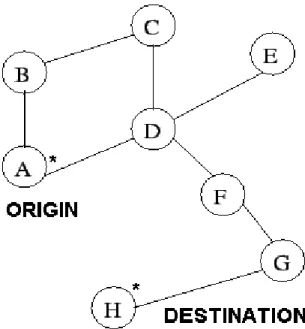
(35) 2.5. ACTIVE ROUTING. 21. For example, a path network can be organized in a star topology. From the center (imagine Paris) ray-like delivery paths exist toward each possible destination. There are also paths from each node toward the center. For routing, data packets are sent toward the center where they will be redirected to the desired delivery path. Alternatively, we can imagine a fully decentralized configuration where each node is the center of a separate star network from where delivery paths stretch out to each node in the network. The highway analogy seems to imply that the delivery path infrastructure is permanently available, that is, active packets pro-actively maintain full routing connectivity all the time. However, there are also reactive approaches to ad hoc routing where a path is only created when there is actual demand for data delivery (e.g., AODV).. 2.5.4. Conventional Routing vs Active Routing. The principal function of conventional routing is to find a path from the origin node to destiny node inside the network. The most important characteristics of conventional routing are the following: the process of routing has to follow some rules to perform its job, these rules are know as protocols or routing algorithms. Another function of the conventional routing unite the network and the distribution of the user traffic besides generate and have a selection of the optimal route based on the information that are represented in the routing tables. [18] In other hand, with active routing the user of the network has the ability to modify some rules that are defined by the routing protocols, in other words, the routing algorithm perform its job with some modifications in its structure. These modifications give a better performance to the conventional routing protocol and the delivery of packets are more faster improving the delay. To understand a little bit more this difference, we will see a visual example of conventional routing and active routing. The figure 2.7 show us a network where the conventional routing protocol found the optimal path, but in this case we have a problem with a broken link C → D, then, the conventional routing protocol decides to send a packets from C to the origin node with the finality to inform that is necessary find another route. The figure 2.8 shows a network with active routing, this network present the same problem with a broken link C → D, but in this scenario, C decides to create a solution to this problem and find another node that allows us to continue with the packet delivery.

(36) 22. CHAPTER 2. BACKGROUND. Figure 2.7: Example of conventional routing. with out the need to inform the origin. The active routing help us a lot when we talk about parameters like delay of the network, resources and bandwidth. It is very important consider that in the active routing algorithm, every node becomes a router with the decision of the costumer.. Figure 2.8: Example of active routing. Another important advantage that the costumer of the network receives when has the control of the path network is that can improve and upgrade the ZRP network with the finality to compete with others topologies. There are some processing cost on active nodes nodes to get that upgrade, the user of the network will decides if the cost that represent that power of processing is enough to get a better delay, or if the cost is too much expensive for their purpose..

(37) 2.5. ACTIVE ROUTING. 2.5.5. 23. Route Discovery and Route Maintenance. There are two kinds of functions that must be taken in consideration. The selection of the route from the origin node to the destiny node and the delivery of packets to the corresponding destiny, to perform that functions we must consider the following concepts: • Route discovery • Route maintenance All routing protocols depends a lot of the information that save the connectivity of the network, in ad hoc networks every node transmit in a period of time an active packet called beacon to collect information that will help the protocol, the beacons announce the presence of the nodes and find the connectivity of the network. When a call arrives from the origin node to destiny and there is not a path available, the origin node perform a request to find an optimal path.[19] It is very important to have a good routing maintenance in an ad-hoc network, if we have an excellent routing maintenance we have no need to call any route discovery, giving us a better end to end delay, stability in the network, better throughput connection perceived by the application. There are different ways to maintenance a path for ad hoc protocols, for example, if we use a DSR protocol we can implement the following instructions to maintenance the route: when a node transmits a data packet, a route reply or a route error, this node must verify that the next node receive the packet correctly, if not, the node must send a route error to the node that is responsible of generate the header of the path and the origin node makes a new petition to find another route. Some protocols has a simple maintenance for example the AODV protocol. In case of a broken link, this protocol only send a RREP back to the origin with the finality to star a new search. In this thesis work we are going to implement the ZRP protocol, and that why it is good to talk about routing maintenance focus on ZRP protocol. A simple way to maintenance a path in this kind of ad-hoc network is with the implementation of active routing, when we have a path traced by the origin node, we can maintenance that route with intelligent nodes that are involved in the network performance, that nodes has the ability to generate an alternative route defined by the origin. To resume the current chapter, we talk about the different protocols in ad hoc networks with the finality to understand and select the one who is better for our model. We are going to select the ZRP protocol because has proactive and reactive characteristics.

(38) 24. CHAPTER 2. BACKGROUND. and collect different advantages that other protocols don´t have, for example, has good performance when the network has mobility. On the next chapter we are going to explain the implementation of algorithm based on active routing theory, also new concepts that we need to know for a better understanding of the propose model..

(39) Chapter 3 Proposed Model. This chapter contains the description of the active routing model used to improve the performance of the Ad Hoc network based on a ZRP protocol. Packet loss ratio, carried traffic and the average end to end delay are the parameters that we are going to calculate in this work. Active routing has a very good ability to work in scenarios where the nodes on an Ad-Hoc networks has medium an high mobility, therefore, is for this peculiarity that we are going to implement an algorithm with active routing based on multi-path theory that help us to improve an ad hoc network with ZRP. How can we make a MANET more efficient with active routing?. The answer is have nodes more intelligent and efficient inside the net. For this thesis work, our nodes has the ability to change the routing table in cases of conflict or broken links, creating a multi-path that will generate a different route to already established, with out the need to send the information of that broken link to the origin node. The first issue that we have to implement is a simple scenario with 10 nodes and 0 mobility, see figure 3.1. With the finality to understand the behavior of our network using ZRP. The protocol ZRP, works in two stages that is characterized by the hybrid protocols. In our thesis work, when the origin node has like a neighbor (stage of IARP)the destiny node, the first one is going to deliver the packets with out the need of any active routing implementation. The second stage that characterizes the ZRP protocol is when the node origin has not a direct communication with the destiny, so is when the Interzone routing protocol(IERP) takes some action. See figure 3.2. The IERP protocol start looking for multiple routes that communicate the node origin and destiny node. In this figure we can see some of the 25.

(40) 26. CHAPTER 3. PROPOSED MODEL. Figure 3.1: Network with 10 nodes. routes, for example the route 1 → 2 → 10 is the route that has the minor number of hops.. Figure 3.2: Network Using ZRP protocol.

(41) 3.1. MOBILITY MODEL. 3.1. 27. Mobility Model. We implement a uniform random distribution in an area of 1000 square meters to get the initials node positions. The direction of the nodes is established also with a uniform distribution between 0 to 2π. How can we get the velocity V of the node and the new position? the answer is showed in the formulas below.. V = Vx + Vy. (3.1). where V x is the component for the horizontal velocity in a plane, and V y correspond to the vertical velocity. The new position of each node is given by the next equation.. Xx = Vx ∗ t + X0. (3.2). Xy = Vy ∗ t + Y0. (3.3). where Xx and Xy represent the horizontal position and the vertical position respectively. The variables X0 and Y0 represent the the position of the node at the beginning of the simulation or the initial position. See fig 3.3 as an example of mobility with medium and high mobility.. 3.2. Beacon Packets. A beacon packet (also called HELLO packet) is a special packet with a message that is sent out periodically from a router or node to establish and confirm network adjacency relationships. On networks capable of broadcast or multicast transmission, a HELLO packet can be sent from a node simultaneously to other nodes to discover neighboring nodes. Another target of these packets is to give the information to each node in the network about other nodes with the actualized routing table. When the hello packet are received for a new neighbor, the routing table is actualized, so this way, the network are always finding and refreshing the position of the nodes..

(42) 28. CHAPTER 3. PROPOSED MODEL. Figure 3.3: Network with mobility. 3.3. Shortest Path Routing. The following method is used in many forms, because it is simple and a little bit easy to understand. The principal idea is to build and graph an ad hoc network with N nodes. To choose a route between a given pair of nodes (node 1 to N), the algorithm just finds the shortest path between them on the graph. The shortest path concept includes definition of the way of measuring path length. Deferent metrics like number of hops, geographical distance, the mean queuing and transmission delay of the node can be used. In the most general case, the labels on the links could be computed as a function of the distance, bandwidth, average traffic, communication cost, mean queue length, measured delay, and other factors. There are several algorithms for computing shortest path between two nodes of a graph. The algorithm that we are going to implement in this thesis is the Dijkstra algorithm.. 3.3.1. Dijkstra Algorithm. The Dijkstra’s algorithm is easy to understand. We find the cheapest route from one place to another by finding the cheapest route to every place on a network node by node. We do this by applying a simple method over and over again, until we run out of places to find the cheapest route. See figure 3.6.

(43) 3.3. SHORTEST PATH ROUTING. 29. Figure 3.4: An example with a simple Dijkstra. There are four nodes on this network, named A, B, C and D. They are connected by links that cost different amounts to use: We want to find the cheapest way of delivering pakets from A to D. There are various routes the data could use to get from A to D. Dijkstra’s algorithm lets you work out the cheapest way, no matter how complicated the network is. We going to see how much it costs to get to the computers directly connected to node A. It costs 3 to get to B, and 2 to get to C. Now we choose the smallest temporary label on the network, and make this permanent. This is the 2 label on node C. Then we work out how much it costs to go to each node connected to C. The node C is connected to A, but we already know the cheapest route to A (it has a permanent label already), so we can ignore this one. To get from A to B via C costs 4 (2 to get from A to C, and 2 more to get from C to B). This is the same as going directly from A to B, so we can ignore this route too. C is also connected to D, and this will cost 8 in total, so D gets a temporary label of 8. Then we do the whole thing again. We find the smallest temporary label on the network (the 3 label on B) and make it permanent. Then we look at all the nodes connected to B and work out how much it will cost to get to them. If the new cost is the same or more than the label on the node, we ignore it. However, if the new cost is cheaper, then we update the label. So, as the route A → B → D only costs 7, and this is cheaper than the A → C → D route that cost 8, we can update the temporary label on D from 8 to 7. See figure 3.7 to check the shortest path routing..

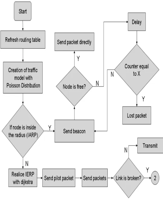
(44) 30. CHAPTER 3. PROPOSED MODEL. Figure 3.5: Example solved with Dijkstra algorithm. In this work we are going to assume a cost uniform for every link, this way we are going to find de shortest path depending on the number of hops. It is more efficient work with the number of hops when our network has too much mobility.. 3.4. Active Routing Algorithm. The active routing algorithm is divided in two simples algorithms to get a better understanding and clarity about we are planning to do.. • Shortest path routing,creates the route that a packet is going to take, besides, decide if a packet is transmitted or wait for the creation of an alternative route. • Multi-path diagram, create a new route that the packet will follow to de destiny.. 3.4.1. Shortest path routing Diagram. This part is represented by a block diagram in figure 3.8. Is the part of the algorithm that creates our network with uniform distribution, refresh the routing table for each node and implement a traffic model with poisson distribution. Also implement an Ad-Hoc network using ZRP. If the source and the destiny are neighbor, the origin node send a beacon to ask if the destiny is free to receive the packets. In case that the destiny is busy, the source not transmit the packet until the destiny is free.

(45) 3.4. ACTIVE ROUTING ALGORITHM. 31. Figure 3.6: Block diagram of shortest path routing. or too much time has passed. If the source and the final node are not neighbor. The algorithm implement a search to find the optimal path (shortest path routing with dijkstra). When the optimal path is founded, the algorithm send pilots packets with the purpose of inform each node in the universe which one is the origin node, and which one is the final node, with this action we have no need to inform to the origin node when a link is broken or has some failures, let.

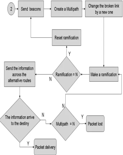
(46) 32. CHAPTER 3. PROPOSED MODEL. us gain a lot of time, optimized resources and bandwidth. When the pilot packet are already sent, we finally send the packets trow the optimal path, in case that the connection is down caused by the mobility of the nodes, the algorithm decides call for a new algorithm of multi-path.. 3.4.2. Multi-path Diagram. The ability of creating multiple routes from a node origin to a destiny node is implemented to give us a backup or alternative route. When the primary route has not success to deliver the packets in some way, the alternative is implemented. This give us a very good fault tolerance in case of efficient recovery from route failures. Distributing traffic among multiple routes exploits availability of network resources to increase throughput and reduce delay,[15][16]. This part of the algorithm is showed with a block diagram in figure 3.9. When a node detects that its next hop (given by the routing table) is not in its coverage area, this node send beacons packet to discovery the neighbors in that moment. When the new neighbor has been detected, the node creates a multi-path with the finality to change the broken link by a new one. The new node in the route check its neighbors with the finality to find the node that have the old route. For example in fig 3.10 The original route is A → B → C, but the link AB is broken, so the algorithm create a new route (multi-path), A → D, in that moment D checks their neighbors an if find C, recover the route that was planned by the dijkstra algorithm. If we continue with the explanation of the flow chart, we can see the part of the ramification diagram. In our model we proposed to make 2 ramification with the finality to have a limited point of search. When our model creates a multi-path also creates a ramification, in case that D does not find C, creates another ramification with E looking for C. In case that the second ramification does not find the route to the destiny, our model has the ability to create a new multi-path, also with 2 ramifications. We decide how many multi-paths our networks can generate. When the new route is already traced, the algorithm decides to send the information across the nodes, then, we check if the information arrives to the destiny. If the answer is.

(47) 3.5. EFFECTS OF THE PHYSICAL LAYER IN OUR MODEL OF ACTIVE ROUTING33. Figure 3.7: Block diagram of multi-path. affirmative. the node deliver the packet, and if the answer is negative we have the option of generate a new multi-path or declare a packet lost.. 3.5. Effects of the Physical Layer in our model of Active Routing. When we talk about the effects of physical layer we are refereing to the concept of antennas. The antennas are dispositive that are used to receive and transmit microwave signals. A very important point to consider when we talk about the antennas is the attenuation of.

(48) 34. CHAPTER 3. PROPOSED MODEL. Figure 3.8: Example of one multi-path with one and two ramifications. Figure 3.9: Example of 1 multi-path with one ramification. Figure 3.10: Example of 1 multi-path with 2 ramifications.

(49) 3.5. EFFECTS OF THE PHYSICAL LAYER IN OUR MODEL OF ACTIVE ROUTING35 the signal. There are two factors that attenuate the signal.. • The attenuation caused by the air • The dispersion of the signal caused by the transmission form To differentiate the form of transmission there are two kinds of antennas, the omnidirectional and directional antennas. The omnidirectional antennas are capable of radiate energy in all directions, an example of this antennas is the isotropic antenna. The habitual use of the real omnidirectional antennas makes that the antenna not irradiate the same energy in all directions, in fact, there are a zone where the energy is equal, for example in the horizontal plane. The directional antennas are those that have been conceived and constructed with a important finality, most of the energy is broadcast in a direction in concrete. It can present a case when we desired to transmit in several directions, but always we will be speaking of a number of certain directions, where were the main lobe and the secondary ones. If the nodes of our ad hoc active network handle directional antennas instead of omnidirectional, the network in questions would become more efficient in concepts like power, mainly in the ends of the area of the neighboring nodes, besides as the directional antennas has the ability to broadcast in different directions we can have detected different neighbor nodes. Another advantage that give us the directional antennas is the trustworthiness or reliability, if we spread the information in all the directions when really a single one we want to arrive at, we have more dangers of the confidential data because it can be caught by someone that it does not interest to us. Another advantage that the directional ones give us on the omnidirectional is the saturation of frequencies, since if we used a frequency in a very straight way between two antennas, we obtained the rest of the space available for that same frequency..

(50) 36. CHAPTER 3. PROPOSED MODEL.

(51) Chapter 4 Numerical Results This chapter shows the results obtained with de model described in chapter 3 from the implementation of active routing in a wireless ad hoc network using ZRP. The parameters and the considerations that we take in the simulation of the algorithm and network are also presented in different scenarios.. 4.1. Proposed scenarios. In this section we propose different types of scenarios, to describe better the performance of our simulation. For all the scenarios the simulation program was written in Matlab version 6.5 to simulate the algorithms in wireless ad ad hoc networks using ZRP. The scenarios are:. • Scenario 1.- In this scenario we compare the packet loss ratio with respect of time This scenario has not mobility performance • Scenario 2.- The objective of this scenario is to compare the packet loss ratio with our different implementations (ZRP, multipaths and ramifications). This scenario has medium mobility performance • Scenario 3.- This scenario has very high mobility, we compare the the packet loss ratio for our different cases. For every scenarios we are going to calculate others parameters like carried traffic and the average end-to-end delay. For example, we are going to compare how our model behaves when check the end-to-end delay parameter with different λ’s.. 37.

(52) 38. CHAPTER 4. NUMERICAL RESULTS. Packet loss ratio is the relation between the total number of packets blocked and the total number of packet generated during al the simulation process[17]. Carried traffic CT is defined by the formula below, where P ktb and P ktg are the packets blocked and generated during the simulation process respectively. We consider λi as the rate of packets in node i in a Poison traffic process, and µi is the value of the exponential distribution of service period of time in node i.. CT = (1 −. 4.1.1. P ktb X λi )( ) P ktg i µi. (4.1). Scenario 1. In this analysis we consider the parameters shown in table 5.1 which are used to calculated the metrics that we are going to obtain and compare.. Table 4.1: Parameters for ZRP implementation with zero mobility Parameter. Value. Nodes Mobility Coverage ratio per node Coverage area Time of simulation Normal average call arrival rate λ High average call arrival rate λ Velocity of the packet Velocity of buffer. 150 nodes No mobility 12 mts 100m x 100m 50 units (virtual time) 7pkt/time 10pkt/time 300 x 106 mts/time .0100 mts/time. Note. The number of packets generated in one time step follows a Poisson distribution with rate λi for node i. We can see in Figure 4.1 and 4.2 that the packet loss ratio has better performance while we increase the number of ramification, if we use a network with pure ZRP, the probability of blocking is greater that if we use a multipath with one ramification. Even better, if we implement an active network with one multipath and 2 ramification, the performance.

(53) 4.1. PROPOSED SCENARIOS. 39. Figure 4.1: Packet loss ratio with no mobility and λ = 7. Figure 4.2: Packet loss ratio with no mobility and λ = 10. of the network has a better improvement. In the table 4.2 we can observe the results in percents, if we consider the greatest.

(54) 40. CHAPTER 4. NUMERICAL RESULTS. Figure 4.3: Carried traffic with no mobility and λ = 7. Figure 4.4: Carried traffic, no mobility and λ = 10. percent of lost using the ZRP algorithm, we can observe at the moment of using multipath with only one ramification we got a percent of improvement of 23.19% and 64.04% when we implement the algorithm with 2 ramifications. Also, we can check that the percent of.

(55) 4.1. PROPOSED SCENARIOS. 41. improvement with respect to multipath with 1 ramification is 53.18%. Table 4.2: Improvement of Packet Loss Ratio with no mobility and λ = 7 Algorithm ZRP Multipath Two Ramifications. Packet loss ratio 0.2147 0.1649 0.0772. Against ZRP 23.195% 64.043%. Against Multipath 53.184%. Note. The value of the packet loss ratio that we are using in this table correspond to the value calculated in the last iteration of my program, because this calculated value is the average of all my entire simulation. If we check the table 4.3, we can see, that also are an improvement in the results consulting the parameter of traffic load.. Table 4.3: Improvement of Carried traffic with no mobility and λ = 7 Algorithm ZRP Multipath Two Ramifications. Carried traffic 0.7649 0.8343 0.9259. Against ZRP 9.073% 21.048%. Against Multipath 10.980%. If I have a minor packet loss ratio we get a greater percent of favorable traffic for any network in general. It can be observed that if we use a multipath with 1 ramification, the % of improvement is 9% and if we utilize the algorithm with 2 ramifications the improvement is 21% with respect the ZRP protocol. Also, we can check that the percent of improvement with respect to multipath with 1 ramification is 10.98%. All the values above was resulted when the is 7 packet per time unit.. 4.1.2. Scenario 2. To study this scenario we implement the same parameters that we used in table 4.1. In this scenario we employ the topology of scenario 1 but we change some parameters to analyze the behavior of the network, which are mobility of the nodes..

(56) 42. CHAPTER 4. NUMERICAL RESULTS. The table 4.4 show us the results, we can observe that if we use the algorithm with multipath with one hop, we got a value of 28.97 % and 51.43 % when we implement the multipath algorithm with 2 hops. Again, we can observe that the percent of improvement with respect to multipath with one hop is 31.62 %. Figure 4.5: Packet loss ratio with medium mobility and λ = 7. Table 4.4: Improvement of Packet Loss Ratio with medium mobility and λ = 10 Algorithm ZRP Multipath Two Ramifications. 4.1.3. Packet loss ratio 0.4394 0.3121 0.2134. Against ZRP 28.9713% 51.433%. Against Multipath 31.624%. Scenario 3. In this analysis we consider the parameters shown in table 5.1 This scenario has very high mobility, we compare the the packet loss ratio for our different cases, and the carried traffic. It can be observed that if we use a multipath with 1 ramification, the % of improvement is 11.56% and if we utilize the algorithm with 2 ramifications the improvement is.

(57) 4.1. PROPOSED SCENARIOS. 43. Figure 4.6: Packet loss ratio with medium mobility and λ = 10. Figure 4.7: Carried traffic with medium mobility and λ = 7. 21.52% with respect the ZRP protocol. Also, we can check that the percent of improvement with respect to multipath with 1 ramification is 8.923%..

(58) 44. CHAPTER 4. NUMERICAL RESULTS. Figure 4.8: Carried traffic, medium mobility with λ = 10. Table 4.5: Improvement of Carried traffic with medium mobility and λ = 10 Algorithm ZRP Multipath Two Ramifications. Carried traffic 0.5613 0.6791 0.7766. Against ZRP 20.986% 38.357%. Against Multipath 14.357%. If we check the behavior of the plots for all scenarios, we can observe the packet loss ratio has an improvement and better performance, because we have more packet delivery in a success status. Also, the carried traffic that support our networks with ZRP is better when the application of the algorithm is implemented..

(59) 4.1. PROPOSED SCENARIOS. Figure 4.9: Packet loss ratio with high mobility and λ = 7. Figure 4.10: Packet loss ratio with high mobility and λ = 10. 45.