Asymptotic stability of a mathematical model of cell population Mihaela Negreanu , J. Ignacio Tello

Asymptotic stability of a mathematical model of cell population

Mihaela Negreanu , J. Ignacio Tello

A B S T R A C T

We consider a simplified system of a growing colony of cells described as a free boundary problem. The system consists of two hyperbolic equations of first order coupled to an ODE to describe the behavior of the boundary. The system for cell populations includes non-local terms of integral type in the coefficients. By introducing a comparison with solutions of an ODE's system, we show that there exists a unique homogeneous steady state which is globally asymptotically stable for a range of parameters under the assumption of radially symmetric initial data.

1. Introduction

The growth of cells colonies has been a focus of research since the first studies of cancer. With the increasing number of experimental data have appeared a large hierarchy of mathematical models. In this paper, we consider a simplified mathematical model in a free boundary domain. The system simplifies the problem proposed in [9] based on a continuous distribution of cell population and modeled by hyperbolic equations.

Systems of hyperbolic equations in that context have been used before by several authors (see for instance Friedman [2,1], Friedman and Tao [3], Tao [8] and references therein).

We denote by "s" the density of a colony of cells in a bounded domain Q(i) with moving boundary "(9i?(£)". We assume that the cells die at constant death rate A;s. The dead cells are removed at constant

rate k<i as they decompose at rate k'd assumed constant. For technical reasons we take

kd > | - (1-1)

The volume is composed by the living cells and death cells and it is exemplified as a porous medium with a radial distribution in a spherical domain. The flow velocity in the interior of the colony is denoted by ' V

+ V • (vs) = kss - kds, 0 < t < T, x e f2(t), and the density of death cells by d. After renormalization we may assume

kd = kd

and the problem is described by the following system of equations

ds ~di dd

— + V • (vd) = kds - kdd, 0 < t < T, x e O(t) (1.2)

with regular initial data.

The growth factor depends of the total mass of living cells and it is defined by

ks = 1

-\mi

s

n(t)

The coefficient represents the balance between the constant birth rate and the death rate caused by the limited resources. We consider that the resources depend of total amount of population \nlts\ Jnrt\ s and have a constant distribution in the domain.

We assume that the density of cells into the colony is constant, i.e.,

s + d = l. (1.3)

Adding both equations we have that

V-v = kss-kdd. (1.4)

We take on radial symmetry and therefore the domain Q(i) is as follows

Q{t) = {x G R3 so that \x\ < R{t)}

where R(t) is the exterior boundary of the tumor. Velocity ' V of the cells at the boundary determines the expansion of the free boundary, i.e.,

The aim of the present paper is to prove that:

Theorem 1.1. For kd > 4/3, there exists a constant steady state

s - i + 2

such that, for any positive and regular initial data so, the solution s of system (1.2) satisfies \\s — s*llr™ - > 0, as t —> oo

II II _L°° ;

The proof is based on a comparison argument adapted to hyperbolic equations. Comparison arguments have been widely used in parabolic systems, see for instance [4-7]. In the next section we construct a coupled system of ODE's to obtain a sub- and super-solutions of the hyperbolic equation (Lemma 2.4). The asymptotic behavior of the sub- and super-solutions (Lemma 2.3) is the final step to prove the theorem.

2. Mathematical analysis

We introduce the spacial variable r £ I := (0,1) with formula as follows \x\ r := R(t) Since v ds V • (vs) = sV • v + v • Vs = s(kss — kdd) + -^77-Ror and 1 ks = l - j m J s = l - 3 / r 2s , (2.5) Q{t)

thanks to (1.3), the system (1.2)—(1.4) becomes ds ( R v \ ds

1- — r 1 — =

a

l ^

i U i =

'-'

-

' '''•<>'

d_

dr

(r

^]=r

((k

+ k

)s-k

), (2.7)

where A;s is defined in (2.5). The system is completed with the initial data so := s(r,0) and the boundary

condition obtained by integration in (2.7).

We consider the auxiliary system of ODE's given by

s' = s(l-s)-s2(l + kd-s), 0<t<T, (2.8)

s'= s(l-s)-s2(l + kd-s), 0<t<T, (2.9)

with positive initial data so and so, respectively.

Lemma 2.1. Assuming that

0 < so < so < 1, (2.10)

the solution to (2.8)-(2.9) exists globally in time and satisfies

0 < s < s < 1.

Proof. Since on the right hand side of the equations the functions are regular, we have existence and

uniqueness of solutions in a maximal interval (0, Tmax), where Tmax satisfies

lim t + \s(t)\ + \s(t)\ = 00

and

t + \s(t)\ + \s(t)\ < oo, for any t < Tmax.

Now, we take the first to > 0 such that either

(1) s(tQ) = 0,

(2) s(t0) = 1,

(3) s(t0) = s(t0)

or any combinations of the previous cases. We argue by contradiction and take for granted that (3) occurs. Then s'(to) = s'(to), we consider the ODE

u' = u(l — u) — u2(l + ka — u), t > to, u(to) = s(to) = s(to),

which has a unique solution. Notice that s = s = u is the solution to the system (2.8), (2.9) with initial data s(to) = s(to) = u(to). By uniqueness of solutions, s = s for any t G (0,Tmax), which contradicts (2.10). If s(to) = 1, then s'(to) ^ 0 and we have that

0 < 1 - s - kd

which contradicts (1.1). If s(to) = 0, by uniqueness of solutions we have that s = 0 for any t G [0,Tmax)

which contradicts (2.10). Finally, the solution is uniformly bounded and exists globally, i.e. Tmax = oo. •

Lemma 2.2. Let s* = 1 + (kd — (k% + 4kd)*)/2, then assuming

so < s* < so, (2.11) it leads us into

s < s* <s,

where (s,s) satisfies (2.8)-(2.9), with initial data

(s_o,s~o)-Proof. As in the previous lemma, we argue by contradiction. Assume there exists to < oo such that s(to) = s*,

s(t)<s* and s(t) > s*, t<t0. (2.12)

Notice that, by Lemma 2.1 we have that s(to) < s(to) = s*. Since s* satisfies

l-s*-s*(l + kd-s*) = 0 , we obtain

s'(to) = s*(s* -s) > 0

which contradicts (2.12) and proves s(to) > s*.

Lemma 2.3. Let us consider hypotheses (1.1), (2.10) and (2.11). Then, we have s > s*s_o/so and

|s — s| —> 0, as t —>• oo.

Proof. We divide (2.8) by s and (2.9) by s to obtain

jt log -s = -kd(s -s) + {s2 - s2) = ((s + s) - kd)(s - s). (2.13)

By Lemma 2.1, it results in

u ^ , * u o , kd ~ Vkj + 4kd -kd- ^k2 + 4kd

s + s-kd^l + s -kd = 2-\ W~Y kd = 2 -\ ^—^ := - e0.

Notice that, by (1.1) we have eo > 0. We now follow the proof in [10], and thanks to (2.13)

^ l o g ^ - e o ( s - s ) . (2.14) Thanks to Lemma 2.1 we have that s — s ^ 0 and therefore

d , s

- log - < 0. at s

After integration we obtain

which implies and iog - ^ log — s s0

1

< £°

We now apply the Mean Value Theorem to (2.14) to obtain

d s ( s \ ( s~ — log - ^ - e0( s - s) ^ - e0 exp f log - j ^ -e0£(£) f log

-for £(£) G (s(t),s(tj). Thanks to (2.15) and Lemma 2.1 we have

d , s . * so A s

— log - ^ - e0s — log -at s so V s

After integration we obtain log - ^ e so log s s0 and *o**f£t, *o ^ exp\ e ° 5o log so

Thanks to (2.15) we have that

\s — s \ = s <s* ^s* _{exp< e} - t0s ^ t | SO

SO

0 as t —> oo

and the proof ends. •

Lemma 2.4. Under assumption

0 < So ^ So ^ so ^ 1, (2.16)

the solutions to (2.8)-(2.9) and (2.6)-(2.7) satisfy

s ^ s ^ s, /or £ > 0. (2.17)

Proof. The proof of the lemma presents some technical differences with standard comparison arguments,

mainly because the integral factors. To solve such problem we introduce the following auxiliary function

{

s if s ^ s.

We replace s by <f>(s) in the integral terms of the system and once we prove the lemma, we may eliminate <f>. We consider the following functions

S = s — s, S = s — s. Notice that S satisfies the equation

dS ( R v\dS h —r 1 dt V R R \-^ = (ks- kd)S - S((ks + kd)s - kd) -s((ks + kd)s - ks + 1 - s - s(l + kd - s)) (2.18) Moreover we have -s((ks + kd)s -ks + l-s-s(l + kd-s)) =-s U l + kd)S + 3 I r2 (<f>(s) - s) - 3s I r2(j)(s) + s2 J ^-s(l + kd-s)S.

We introduce the function He defined by

f if x > e

He(x) := <( f if 0 < x < e 0 if x < 0.

Multiplying (2.18) by r2He(S) and integrating over I, by taking limits as e —> 0, we get

d

at •

' ' "

I I

(

_r

l

+

i)i^

=

l

r2s+

\-

{ks

~

kd)s

~

s

^

{ks+kd)s

~

k

^

r2S+7s(l + kd-7s). (2.19)

i

The second term in the left side of (2.19) is treated in the following way 2f R v\dS+ nR f 2-, [-, 1 dr2v

r - r — + — — ± = 3— / r2S+ - / S

R RJ dr RJ ^ J ^ R dr

i I I

Thanks to (2.7) the last term in the previous equation is simplified to

r2S+ —--— = - / r2S+ {(ks +kd)s- kd) (2.20) r2R dr i i resulting in

!/

r25

+«H+

c

)/

r25

By Gronwall's Lemma we obtain that s ^ s as far as RR~X is bounded. In the same way we obtain s ^ s. To end the demonstration we claim that RR~X is bounded for all t < oo. By contradiction, if there exists

Tmax < oo such that \RR~X\ = oo then

v(l,Tmax) = lim / r2((ks +kd)s- kd) = oo <• ' J max J

I

which contradicts the fact that s ^ s in (0, Tmax) and the testing is done. •

Proof of Theorem 1.1. As a consequence of Lemma 2.3 and Lemma 2.4 we have that

\\s — s* I L o o-^ 0 as £ —» oo

II II _L°°

and R(t) ~ Ro exp(((l — s* + kd)s* — kd)t) and it's proved as right. •

3. Numerical simulations and discussion

We have analyzed a first order system of hyperbolic equations in a moving domain with non-local terms depending on a parameter kd. The system describes a cell's population dynamics related with other

math-ematical models in tumor growth existing in the literature. The results show how the population tends to a homogeneous distribution of cells in the domain as time grows for kd > 4/3. A lower estimation of the

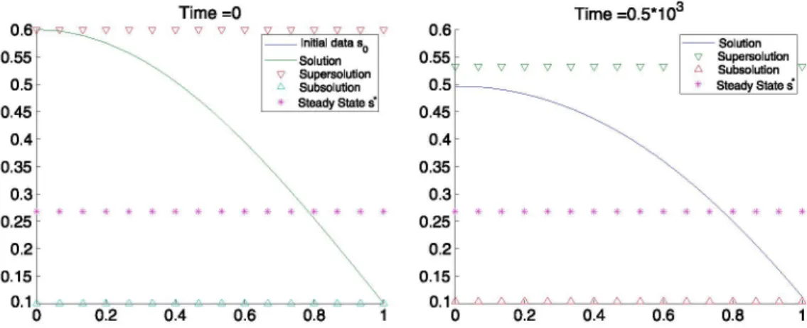
0.6 0.55 0.5 0.45 0.4 0.35 0.3 0.25 0.2 0.15 Time =0 - _ _ V V V V V V V V V V V V V V Initial data s — Solution v Supersolution ^ Subsolution * Steady State s* 0.6 0.55 Time =0.5*103 Solution v Supersolution v v v v v v A Subsolution 0.51= -—____ | Steady State s 0.1& A A A A A A A A A A A A A A-0.2 0.4 0.6 0.8 0.45 0.4 0.35 0.3 0.25" 0.2 0.15 0 l A A A A A A A A A A A A A A A _ ' 0 0.2 0.4 0.6 0.8 1

Fig. 1. Density d i s t r i b u t i o n for t h e solution s (—), t h e sub-solution s ( A ) , super-solution s (V) and t h e s t e a d y s t a t e s* (*) at t = 0 (left) and t = 0.5 • 103 (right).

Time =1.5*10J Time =2*10J 0.4 r 0.35 0.3 0.25 0.2 ^ v v v v v v v v v Solution v Supersolution A Subsolution Steady State s' A A A A A A A A A A A A A A A A 0 0.2 0.4 0.6 0.8 1 0.32 0.3 0.28 0.26 0.24 0.22 0.2 \ ? v v v v v v v v v Solution \7 Supersolution A Subsolution A A A A A A A A A A A A A A A A 0 2 0 4 06 08 1

Fig. 2. Density d i s t r i b u t i o n for t h e solution s (—), t h e sub-solution s ( A ) , super-solution s (V) and t h e steady s t a t e s* (*) at

t = 1.5 • 103 (left) and t = 2 • 103 (right).

rate of convergence in L00(Q(i)) is given by the rate of convergence of the solutions to the associated EDO'

system (2.8)-(2.9).

The following numerical simulations show the convergence of the solution for kd = 2 and how the sub-and super-solutions reach the steady state (see Figs. 1 sub-and 2). Notice that the minimum distance between the maximum of the solution and the super-solution, i.e. \s — maxr € f t(i) s\ is not monotone.

For the remaining cases, when kd ^ 4/3, it is possible that the solutions do not stabilize towards homoge-neous profiles and even non-constant equilibria may appear, but these require entirely different approaches than pursued here where only asymptotic stability is studied.

Acknowledgment

The authors are partially supported by Ministerio de Economia y Competitividad of Spain under grant MTM2009-f3655.

References

[1] A. F r i e d m a n , C a n c e r m o d e l s a n d t h e i r m a t h e m a t i c a l analysis, in: T u t o r i a l s in M a t h e m a t i c a l Biosciences. I l l , in: L e c t u r e N o t e s in M a t h . , vol. 1872, Springer, Berlin, 2006, p p . 2 2 3 - 2 4 6 .

[2] A. F r i e d m a n , C a n c e r as m u l t i f a c e t e d disease, M a t h . M o d e l . N a t . P h e n o m . 7 (1) (2012) 3-28.

[3] A. F r i e d m a n , Y. T a o , A n a l y s i s of a m o d e l of a v i r u s t h a t r e p l i c a t e s selectively in t u m o r cells, J. M a t h . Biol. 47 (2003) 3 9 1 - 4 2 3 .

[4] M. N e g r e a n u , J.I. Tello, O n a p a r a b o l i c - e l l i p t i c c h e m o t a c t i c s y s t e m w i t h n o n - c o n s t a n t c h e m o t a c t i c sensitivity, N o n l i n e a r A n a l . 80 (2013) 1-13.

[5] M. Negreanu, J.I. Tello, On a comparison method to reaction-diffusion systems and its applications to cheniotaxis, Discrete Contin. Dyn. Syst. Ser. B 18 (10) (2013) 2669-2688.

[6] C.V. Pao, Nonlinear Parabolic and Elliptic Equations, Springer, 1992.

[7] C.V. Pao, Comparison methods and stability analysis of reaction diffusion systems, in: Comparison Methods and Stability Theory, in: Lect. Notes Pure Appl. Math., vol. 162, Dekker, New York, 1994, pp. 277-292.

[8] Y. Tao, A free boundary problem modeling the cell cycle and cell movement in multicellular tumor spheroids, J. Differential Equations 247 (1) (2009) 49-68.

[9] J.I. Tello, On a mathematical model of tumor growth based on cancer stem cells, Math. Biosci. Eng. 10 (1) (2013) 263-278. [10] J.I. Tello, M. Winkler, Stabilization in a two-species cheniotaxis system with logistic source, Nonlinearity 25 (2012)