The
Gaia
-ESO Survey: the selection function of the Milky Way field stars
E. Stonkut˙e,
1,2‹S. E. Koposov,
3L. M. Howes,
1S. Feltzing,
1C. C. Worley,
3G. Gilmore,
3G. R. Ruchti,
1G. Kordopatis,
4S. Randich,
5T. Zwitter,
6T. Bensby,
1A. Bragaglia,
7R. Smiljanic,
8M. T. Costado,
9G. Tautvaiˇsien˙e,
2A. R. Casey,
3A. J. Korn,
10A. C. Lanzafame,
11,12E. Pancino,
5,13E. Franciosini,
5A. Hourihane,
3P. Jofr´e,
3C. Lardo,
14J. Lewis,
3L. Magrini,
5L. Monaco,
15L. Morbidelli,
5G. G. Sacco
5and L. Sbordone
16,171Department of Astronomy and Theoretical Physics, Lund Observatory, Box 43, SE-22100 Lund, Sweden 2Institute of Theoretical Physics and Astronomy, Vilnius University, Saul˙etekio al. 3, LT-10222 Vilnius, Lithuania 3Institute of Astronomy, Cambridge University, Madingley Road, Cambridge CB3 0HA, UK
4Leibniz-Institut f¨ur Astrophysik Potsdam (AIP), An der Sternwarte 16, D-14482 Potsdam, Germany 5INAF - Osservatorio Astrofisico di Arcetri, Largo E. Fermi 5, I-50125 Florence, Italy
6Faculty of Mathematics and Physics, University of Ljubljana, Jadranska 19, 1000 Ljubljana, Slovenia 7INAF-Osservatorio Astronomico di Bologna, via Ranzani 1, I-40127 Bologna, Italy
8Nicolaus Copernicus Astronomical Center, Polish Academy of Sciences, ul. Bartycka 18, PL-00-716 Warsaw, Poland 9Instituto de Astrof´ısica de Andaluc´ıa-CSIC, Apdo. 3004, E-18080 Granada, Spain
10Department of Physics and Astronomy, Uppsala University, Box 516, SE-751 20 Uppsala, Sweden
11Universit`a di Catania, Dipartimento di Fisica e Astronomia, Sezione Astrofisica, Via S. Sofia 78, I-95123 Catania, Italy 12INAF-Osservatorio Astrofisico di Catania, Via S. Sofia 78, I-95123 Catania, Italy
13ASI Science Data Center, via del Politecnico SNC, I-00133 Roma, Italy
14Astrophysics Research Institute, Liverpool John Moores University, 146 Brownlow Hill, Liverpool L3 5RF, UK 15Departamento de Ciencias Fisicas, Universidad Andres Bello, Republica 220, 837-0134 Macul, Santiago, Chile 16Millennium Institute of Astrophysics, Av. Vicu˜na Mackenna 4860, 782-0436 Macul, Santiago, Chile
17Pontificia Universidad Cat´olica de Chile, Av. Vicu˜na Mackenna 4860, 782-0436 Macul, Santiago, Chile
Accepted 2016 April 25. Received 2016 April 25; in original form 2016 March 17
A B S T R A C T
TheGaia-ESO Survey was designed to target all major Galactic components (i.e. bulge, thin and thick discs, halo and clusters), with the goal of constraining the chemical and dynamical evolution of the Milky Way. This paper presents the methodology and considerations that drive the selection of the targeted, allocated and successfully observed Milky Wayfield stars. The detailed understanding of the survey construction, specifically the influence of target selection criteria on observed Milky Way field stars is required in order to analyse and interpret the survey data correctly. We present the target selection process for the Milky Way field stars observed with Very Large Telescope/Fibre Large Array Multi Element Spectrograph and provide the weights that characterize the survey target selection. The weights can be used to account for the selection effects in theGaia-ESO Survey data for scientific studies. We provide a couple of simple examples to highlight the necessity of including such information in studies of the stellar populations in the Milky Way.
Key words: techniques: spectroscopic – surveys – stars: general – Galaxy: evolution.
1 I N T R O D U C T I O N
The Milky Way is just one of hundreds of billions of galaxies that populate our visible Universe. However, it is the one galaxy that we can study in the greatest detail. For example, thanks to
E-mail:[email protected]
spectroscopic surveys over the last few decades our understanding of the chemical evolution of our own Galaxy has increased tremen-dously (for reviews see Freeman & Bland-Hawthorn2002; Feltzing & Chiba2013; Bland-Hawthorn & Gerhard2016). A number of large-scale spectroscopic surveys of stars in the Milky Way have been completed or are underway, e.g. SEGUE (Yanny et al.2009), RAVE (Steinmetz et al.2006), GALAH (De Silva et al. 2015), APOGEE (Majewski et al.2015), LAMOST (Deng et al.2012),
C
Gaia-ESO (Gilmore et al.2012; Randich, Gilmore & Gaia-ESO Consortium2013),Gaia(Perryman et al.2001) or are being planned e.g. WEAVE (Dalton et al.2012), MOONS (Cirasuolo et al.2012) and 4MOST (de Jong et al.2014). These are opening a new path to study formation and evolution of the Galaxy in great detail. All spectroscopic surveys of the Milky Way will suffer from selection effects. For example, the object targeting algorithm employed in the survey will cause selection biases. Therefore we need to design our target selection algorithms to be as simple as possible. This way we can determine how the observed spectroscopic sample represents the stars in the parent stellar population. All selection effects need to be accounted for when we want to extrapolate from the observed volume to the ‘global’ volume of the Milky Way.
There have been several SEGUE papers that have demonstrated the importance of accounting for the observational biases in dif-ferent SEGUE samples. Cheng et al. (2012) examined the obser-vational biases of the main-sequence turn-off stars on low-latitude plates and they stress the importance of the weighting procedure for the proper correction for selection biases. Furthermore, Schlesinger et al. (2012) determined and corrected for the effect of the SEGUE target selection on cool dwarf stars (G and K type). A portion of this sample was also studied and corrected for biases in a different way by Bovy et al. (2012) and Liu & van de Ven (2012). Selection effects are also considered in other analyses of spectroscopic survey data (e.g. RAVE, APOGEE; Francis2013; Nidever et al.2014). In this context, it is important to discuss theGaia-ESO Survey con-struction: how targets are selected; allocated on the spectrograph; and finally – successfully observed.
TheGaia-ESO Survey observing strategy has been constructed to answer specific scientific questions. The full survey includes all major stellar populations: the Galactic inner and outer bulge, inner and outer thick and thin discs, the halo, currently known halo streams, and star clusters. Selected targets consist of early-and late-type stars, metal-rich early-and metal-poor stars, dwarfs, giants, and cluster stars across the evolutionary sequence selected from previous studies of open clusters.
By the end, the survey will have observed with Fibre Large Ar-ray Multi Element Spectrograph/UV-Visual Echelle Spectrograph (FLAMES/UVES) a sample of several thousand FG-type stars within 2 kpc of the Sun in order to derive the detailed kinematic and elemental abundance distribution functions of the solar neighbour-hood. The sample includes mainly thin and thick disc stars, of all ages and metallicities, but also a small fraction of local halo stars. FLAMES/GIRAFFE (GIRAFFE: Medium-high resolution spectro-graph) will observe a statistically significant (∼105) sample of stars in all major stellar populations.
TheGaia-ESO Survey will provide a legacy data set that adds great merit to the astrometricGaiaspace mission by assembling a catalogue of representative spectra for stars whichGaiawill deliver highly accurate proper motions but not detailed spectroscopic in-formation. These combined data will allow us to probe for example the properties of the Galactic disc by looking for traces of past, and ongoing, accretion events.
While theGaia-ESO Survey is currently still completing the ob-serving campaign, there are scientific questions that are already be-ing answered. These cover testbe-ing the nature of the thick disc and its relation to the thin disc (Mikolaitis et al.2014; Recio-Blanco et al.
2014; Kordopatis et al.2015); studying the relationship between age and metallicity, and the spatial distribution of stars (Bergemann et al.2014); identifying the remnants of ancient building blocks of the Milky Way (Ruchti et al.2015); determining the chemical com-position of recently discovered ultrafaint satellites (Koposov et al.
2015); analysing metal-poor stars (Howes et al.2014; Jackson-Jones et al.2014); and determining the chemical abundance distribution in globular and open clusters (Donati et al.2014; Magrini et al.
2015; San Roman et al.2015; Tautvaiˇsien˙e et al.2015).
In this paper, we present the target selection process only for the Milky Way field stars observed in theGaia-ESO Survey and provide the weights that characterize the survey sample.
TheGaia-ESO is a public survey and the stellar spectra are avail-able after observations, while reduced spectra and the astrophysical results obtained by theGaia-ESO analysis teams are available to the general community via public releases through the ESO data archive.1
This paper is organized as follows. In Section 2, we introduce the observational setup of theGaia-ESO Survey. Section 3 describes the methods used to select targets for the Milky Way field observations with FLAMES/GIRAFFE and FLAMES/UVES. The initial target selection for GIRAFFE is presented in Section 4 and for UVES in Section 5. In Section 6, we introduce the final target selection, and in Section 7 the weights used to correct for selection effects, calculated after target selection and allocation. In Section 8, we take a first look at theGaia-ESO Survey iDR4 data and discuss the completeness of the successfully analysed spectroscopic sample. We provide a simple example of the metallicity distribution and how it is affected by the selection effects. We show that the metallicity distribution of the Milky Way field stellar sample observed in theGaia-ESO Survey can be corrected to a distribution unaffected by the selection bias by applying the calculated weights. Finally, in Section 9 we discuss the implications of our results and give concluding remarks.
2 O B S E RVAT I O N A L S E T U P F O R M I L K Y WAY F I E L D S
The observations are conducted with the FLAMES (Pasquini et al.
2002) at the Very Large Telescope (VLT) array operated by the European Southern Observatory on Cerro Paranal, Chile. FLAMES is a fibre facility of the VLT and is mounted at the Nasmyth A platform of the second Unit Telescope of VLT. This instrument has a large 25 arcmin diameter field-of-view (see Fig.1).
One of the three main FLAMES components is a Fibre Positioner (OzPoz) which hosts two plates. While one plate is observing, the other plate is configuring fibres so that they are positioned for the subsequent observation. This limits the overhead between one ob-servation and the next to less than 15 min, including the telescope preset and the acquisition of the next field. The fibre facility is equipped with two sets of 132 and 8 fibres to feed two different spectrographs GIRAFFE and UVES, respectively.
The medium resolution spectrograph GIRAFFE with the two setups – HR10 (λ = 533.9–561.9 nm, R ∼ 19 800) and HR21 (λ=848.4–900.1 nm,R∼16 200) was used to observe the Milky Way field stars. To observe Milky Way field stars in high-resolution mode, the survey used the UVES with a setup centred at 580 nm (λ=480–680 nm,R∼47 000; Dekker et al.2000).
3 TA R G E T S E L E C T I O N M E T H O D S
The Gaia-ESO Survey is designed to select and observe three classes of targets in the Milky Way – field stars, candidate mem-bers of open clusters and calibration standards (Gilmore et al.2012;
1http://archive.eso.org/wdb/wdb/adp/phase3_spectral/
Figure 1. The plot shows stars in one of theGaia-ESO Milky Way field, GES_MW_142000-050000. Small dots are surrounding stars, while the large dots are stars involved in the calculation of the selection function (see Section 6 for details). Green thin line – a 1-deg (diameter) field-of-view; red dashed line – a 35 arcmin (diameter) field-of-view; blue solid line – final target selection with a 25 arcmin (diameter) field-of-view (i.e. that at FLAMES on VLT).
Randich et al.2013). In this paper, we present theGaia-ESO Sur-vey selection function only for the Milky Way field stars observed with the GIRAFFE and UVES spectrographs at VLT, not including the bulge. All targets were selected according to their colours and magnitudes, using photometry from the VISTA Hemisphere Survey (VHS; McMahon et al.2013) and the Two Micron All-Sky Survey (2MASS; Skrutskie et al.2006). Selected potential target lists were generated at the Cambridge Astronomy Survey Unit (CASU) centre. We discuss the initial GIRAFFE and UVES target selection and photometry used in more detail in Sections 4 and 5. In the following section, we present the basic scheme constructed to select Milky Way field targets.
3.1 Basic target selection scheme
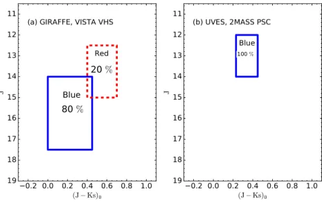
The primary goal of the selection strategy of the survey is to se-lect Milky Way stars in order to study a robust sample of all major Galactic components (i.e. thin and thick discs, and halo). The ba-sic target selection is built on stellar magnitudes and colours. The targets are selected to sample the main sequence, the turn-off, and the red giant branch stars centred on the red clump. To achieve this the stars are selected from two boxes, the blue and the red (see Fig.2a). The blue box is used for the selection of the turn-off and main-sequence targets to be observed with GIRAFFE. The red box is defined to select stars on the red clump or nearby the red clump in the Colour Magnitude Diagram (CMD). For the selection of stars to be observed with UVES only one box is used (see Fig.2b).
The main GIRAFFE target selection is as follows:
Blue box :
0.00≤(J−KS)≤0.45;
14.0≤J≤17.5. (1)
Red box :
0.40≤(J−KS)≤0.70;
12.5≤J≤15.0. (2)
The main UVES target selection is as follows:
Blue box :
0.23≤(J−KS)≤0.45;
12.0≤J≤14.0. (3)
HereJ,KSmagnitudes in equations (1), and (2) are from VISTA VHS photometry and in equation (3) they are from 2MASS pho-tometry. The colour boxes will be corrected for reddening, as de-scribed in Section 3.2.3. The selection algorithm is configured to assign approximately 80 per cent of the targets to the blue box and
∼ 20 per cent to the red box for GIRAFFE (see Fig. 2a for the GIRAFFE observations). All the targets that are in the UVES
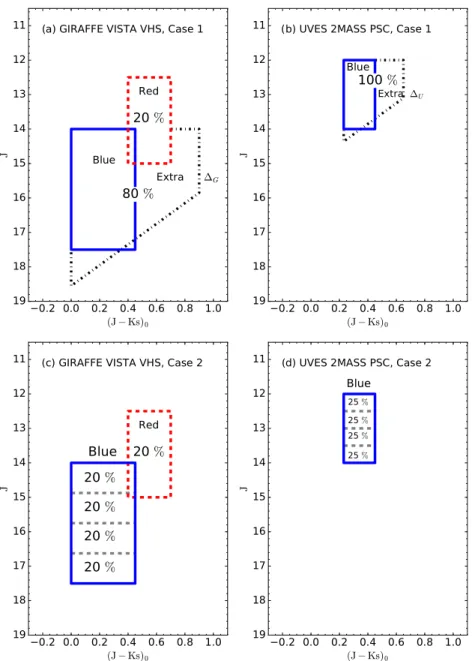
Figure 3. The actual target selection colour–magnitude schemes: (a) and (c) for GIRAFFE, and (b) and (d) for UVES. Target selection based on Case 1 are shown in (a) and (b), and on Case 2 in (c) and (d), respectively. Blue solid line shows the area of targets assigned to the blue box; red dashed line – to the red box; and black dash–dotted line shows the area of second priority targets assigned to the extra box. The right-edge limit (a)Gand (b)Uin Case 1 of the
extra box varies from field to field. The blue box in (c) and (d) for Case 2 is divided into four equal-sized magnitude bins (in order to have the same number of targets per magnitude bin). On thex-axis we show the dereddened (J−Ks)0colour, whereas on they-axis we show the observedJmagnitude (for more details see Section 3.2.3).
selection box area shown in Fig.2(b) were assigned as potential targets for UVES.
3.2 Actual target selection schemes
We divide the selection of stars in the Milky Way fields into two cases, which are described in the following sections.
3.2.1 Case 1
Case 1, which depends on the stellar density, occurs when the field does not have enough targets to fill the FLAMES fibres (e.g. high latitude Milky Way fields). Figs3(a) and (b) show the actual target selection colour–magnitude schemes for Case 1 for GIRAFFE and UVES, respectively. The target selection algorithm is then extended at the right-edge of the blue boxes (see black dash–dotted box in Figs3a and b, and equations 4 and 5), allowing for the selection
of second priority targets. We select second priority targets in the extra box only when all targets in the blue box have already been selected. In addition, in this case the second priority objects were selected with a colour-dependentJmagnitude cut to avoid too faint targets, which would lead to low signal-to-noise ratios (S/N) in the optical spectra. This allows us to also extend the box to slightly fainter magnitudes (see Figs3a and b).
The second priority target selection in Case 1 for GIRAFFE is as follows:
Extra box :
0.00≤(J−KS)≤0.45+G;
J≥14.0;
Figure 4. The frequency distribution of extensionsGandU(see Sec-tion 3.2.1). The dashed line show the right-edge extensionsGfor GIRAFFE and solid line show the right-edge extensionsUfor UVES in Case 1 Milky Way fields.
And for UVES:
Extra box :
0.23≤(J−KS)≤0.45+U;
J≥12.0;
J+3.0∗((J−KS)−0.35)≤14.00. (5)
HereGandUare the right-edge extensions of the extra box for GIRAFFE and UVES, respectively (see black dash–dotted line in Figs3a and b). Furthermore, these extensions vary slightly from field to field. The values for each field are shown in Fig.4and listed in Table1.
3.2.2 Case 2
Case 2 is encountered when the density of stars exceeds the number of fibres available. This algorithm is applied to the Milky Way fields near to the Galactic plane. In Case 2, the target selection algorithm selects targets in such way as to have the same number of targets per magnitude bin (i.e. not to have a bias towards very faint stars). Therefore, the blue box is divided into four equal-sized magnitude bins, withJ1,2,3,4=(Jmax−Jmin)/4, whereJ1is the bright limit, and J4is the faint limit of theJmagnitude (see Figs3c and d). In this case, we have no priorities for what to select within each given sub-box, so the choice is approximately random. We select approximately the same number of stars in each sub-box. The target selection magnitudes and colours for Case 2 follow the same selection limits as presented for the main target selection (see equations 1–3).
3.2.3 Extinction and colour range
The Milky Way fields located near the Galactic plane often suffer from considerable interstellar extinction. TheGaia-ESO Survey tar-get selection algorithm takes the line-of-sight interstellar extinction, AV, into account using the Schlegel dust map (Schlegel, Finkbeiner & Davis1998). Schlegel et al. indicate an accuracy of 16 per cent on their map. Although in the near-infrared the impact of extinction, while expected to be low, cannot be neglected, i.e.E(J− KS)= (c.J−c.Ks)∗AV=0.17∗AV, which leads to approximateE(J−KS) =0.10 forE(B−V)=0.20 (Rieke & Lebofsky1985). Here c.J
and c.KSdesignate the extinction coefficients in theJand KSbands (c.J=AJ/AVand c.KS=AKs/AV) (Nishiyama et al.2009).
The line-of-sight interstellar extinction for the GIRAFFE and UVES fields was treated differently. The line-of-sight interstellar extinction was taken into account by shifting the colour-boxes of GIRAFFE targets by 0.5∗E(B − V). Whereas for UVES targets instead the box was extended to the right (i.e. the blue edge stays fixed) by 0.5∗E(B − V). No shift was applied to the GIRAFFE and UVES boxes in the vertical, magnitude, direction. Here,E(J −KS)/E(B−V)=0.5 (Rieke & Lebofsky1985) and we takeE(B −V) as the median reddening in the field measured from Schlegel et al. (1998) maps.
The median extinction estimated in the field was added to the colour boxes for GIRAFFE in the following way:
Blue box :
0.5E(B−V)+[0.00≤(J−KS)≤0.45];
Red box :
0.5E(B−V)+[0.40≤(J−KS)≤0.70];
Extra box :
0.5E(B−V)+[0.00≤(J−KS)≤0.45+G]. (6)
And for UVES:
Blue box :
0.23≤(J−KS)≤0.45+0.5E(B−V);
Extra box :
0.23≤(J−KS)≤0.45+U+0.5E(B−V). (7)
The medianE(B − V) values vary per field and are listed in Table1. The mean of the line-of-sight reddening for theGaia-ESO Survey observed in Case 1 Milky Way field stars never reaches values greater thanE(B−V)=0.10, and for fields near the Galactic plane not greater than E(B− V)= 1.23. The mean line-of-sight reddening value for Case 1 fields is<E(B−V)>=0.03±0.02.
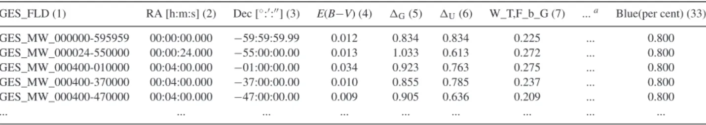
Table 1. Main parameters and weights of the targeted and allocated Milky Way fields. The full table is available online.
GES_FLD (1) RA [h:m:s] (2) Dec [◦::] (3) E(B−V) (4) G(5) U(6) W_T,F_b_G (7) ...a Blue(per cent) (33) GES_MW_000000-595959 00:00:00.000 −59:59:59.99 0.012 0.834 0.834 0.225 ... 0.800 GES_MW_000024-550000 00:00:24.000 −55:00:00.00 0.013 1.033 0.613 0.272 ... 0.800 GES_MW_000400-010000 00:04:00.000 −01:00:00.00 0.034 0.923 0.763 0.275 ... 0.800 GES_MW_000400-370000 00:04:00.000 −37:00:00.00 0.010 0.855 0.785 0.237 ... 0.800 GES_MW_000400-470000 00:04:00.000 −47:00:00.00 0.009 0.905 0.636 0.209 ... 0.800
... ... ... ... ... ... ... ... ...
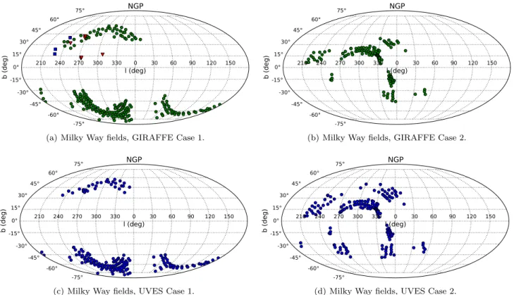
Figure 5. The distribution, shown in Mollweide projection with the Galactic centre in the middle, of the observed Milky Way fields across the sky. (a) and (b) show fields selected based on Cases 1 and 2, respectively, and observed with GIRAFFE. (c) and (d) show fields selected based on Cases 1 and 2, respectively, and observed with UVES. Green circles – fields with the selection based on VISTA VHS photometry; blue circles – fields with the selection based on 2MASS photometry. Additional fields: blue squares – fields with the selection based on SDSS photometry and 2MASS photometry; and red triangles – fields with the selection based on SkyMapper photometry, VISTA VHS photometry and 2MASS photometry (for more information see Appendix B).
For Case 2, Milky Way fields located near the Galactic plane the mean line-of-sight reddening value is<E(B−V)>=0.10±0.12.
3.2.4 Naming conventions
The Gaia-ESO Survey Milky Way field names were created at CASU from the right ascension ‘hms’ and declination ‘dms’ (J2000) of the field centre. For example, theGaia-ESO Survey Milky Way field centred at RA=14h20m00sand Dec= −05◦0000was
as-signed the name GES_MW_142000-050000. The names of the se-lected targets (objects) also encode which selection criteria were used to select them. ‘b’ means the blue box, ‘r ’ the red box, and ‘ e’ is for the extra box (identifies the objects which were added to fill the fibres). Some of the targets were selected by both blue and red boxes, and they have ‘ br ’ in their name.
In the fits headers of the data files the Milky Way fields can be identified with the keyword ‘GES TYPE’. For the Milky Way fields it is set to ‘GE MW’.
3.2.5 The Milky Way field pattern
The distribution of observed Milky Way fields in theGaia-ESO Survey is designed to be well spread. However, the observation range in the Galaxy is restricted to+10◦≥Dec≥ −60◦to minimize the airmass. Fig.5shows the distribution of so far observed fields on the sky. Table2lists the number of observed Milky Way fields in theGaia-ESO Survey up to 2015 June and the number of Milky Way fields in iDR4. For these fields targets were selected as outlined in the preceding sections.
A small subset of additional Milky Way field targets were selected using SDSS and SkyMapper photometry in order to study metal-poor stars and K giants. Some details on the selection of these targets are given in Appendix B.
4 I N I T I A L G I R A F F E TA R G E T S E L E C T I O N
4.1 Photometric catalogue
The survey input and target selection catalogue is the VHS for the Milky Way fields observed with GIRAFFE (McMahon et al.2013). The target selection is based on the panoramic wide field infrared VHS. The VHS survey data consists of three survey components: VHS Galactic Plane Survey (GPS); ATLAS and VHS-Dark Energy Survey (VHS-DES). In particular, catalogue versions from 2011 to 2014 were used to select Milky Way field targets. VISTA VHS has a sufficient sky coverage to meet the full science goals of theGaia-ESO Survey. This catalogue is∼30 times deeper than the 2MASS in at least two wavebands (JandKS) (McMahon et al.2013) (see more about VISTA VHS2). The adopted data quality flags to select Milky Way field targets from the VHS catalogue are listed in Table3.
The target selection magnitude and colour limits for GIRAFFE are presented in Sections 3.1 and 3.2.
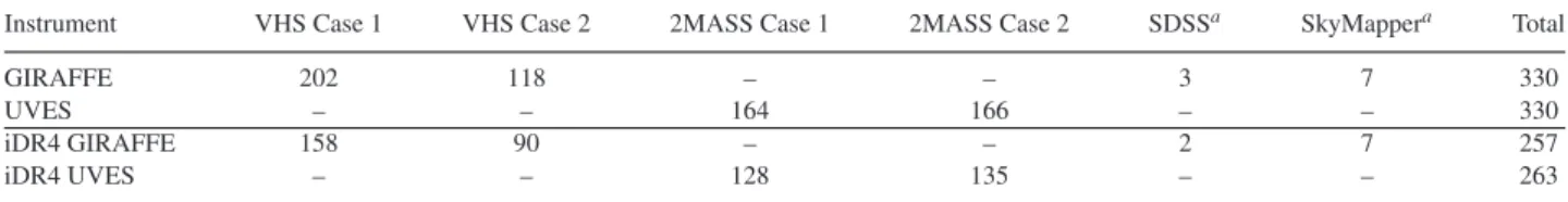
Table 2. The number of Milky Way fields observed in theGaia-ESO Survey up to 2015 June and in iDR4.
Instrument VHS Case 1 VHS Case 2 2MASS Case 1 2MASS Case 2 SDSSa SkyMappera Total
GIRAFFE 202 118 – – 3 7 330
UVES – – 164 166 – – 330
iDR4 GIRAFFE 158 90 – – 2 7 257
iDR4 UVES – – 128 135 – – 263
Note.aSDSS photometry and SkyMapper photometry were used to select additional targets (See Appendix B).
Table 3. Adopted data quality flags for VHS photometry (GIRAFFE) and 2MASS photometry (UVES), and SDSSaphotometry.
Catalogue Requirement Notes
VHS mergedClass mergedClass= −1 Classified as a star.
VHS jAverageConf, ksAverageConf jAverageConf>95,ksAverageConf>95 Average confidence inJ,KSmag. VHS jErrBits, ksErrBits jErrBits=0,ksErrBits=0 Warning/error bitwise flags inJ,KSmag.
VHS Not on the badCCD jx<8000 orjy<12300 Flags used in internal release.
2MASS ph_qual ph qual=AAA Photometric quality flag.
SDSS mode mode=1 Flag indicates primary sources.
SDSS gc type=6 Phototype ingband, 6=Star
Note.aSDSS photometry was used to select additional targets (See Appendix B1).
Figure 6. Colour–magnitude diagrams with VISTA VHS photometry. (a) CMD of the field GES_MW_142000-050000 centred at Galactic longitude l=339◦.9 and latitudeb=51◦.4, and FoV=35 arcmin in diameter. (b) GIRAFFE target selection based on Case 1 selection scheme (see Sec-tion 3.2.1). Blue circles – selecSec-tion of targets in blue box; red squares – selection of targets in red box; and grey stars – second priority targets, respectively.
4.2 Target selection Cases 1 and 2
An example of the target selection for Case 1 is shown in Fig.6. Here, the selected blue circles are targeted turn-off and main-sequence stars to be observed with GIRAFFE, and the red squares are red clump stars. An example of the target selection for Case 2 is shown in Fig.7. For Case 2, the target selection algorithm selected roughly the same number of blue box targets perJmagnitude bin.
As mentioned before, for most of the Milky Way fields the initial target selection algorithm tried to assign 80 per cent of the targets to the blue box and 20 per cent to the red box, respectively. The selection for some of the fields near the Galactic bulge were the only fields where the selection of a blue versus red box fraction was changed, i.e. from 80/20 per cent to 20/80 per cent, to predominantly observe star the Galactic bulge direction, i.e. the red clump stars. Those Milky Way fields are indicated in the last column of Table1.
5 I N I T I A L U V E S TA R G E T S E L E C T I O N
The Gaia-ESO Survey uses UVES with the U580 setup (470– 684 nm) to observe Milky Way field stars. Up to seven separate
Figure 7. Colour–magnitude diagrams with VISTA VHS photometry. (a) CMD of the field GES_MW_201959-470000 centred at Galactic longitude l= 352.◦7 and latitudeb= −34◦.2, and FoV= 35 arcmin in diameter. (b) GIRAFFE target selection based on Case 2 selection scheme (see Sec-tion 3.2.2). Blue circles – selecSec-tion of targets in blue box; red squares – selection of targets in red box, respectively.
objects (plus one sky fibre) can be allocated and observed simulta-neously in the U580 mode. The methodology adopted in theGaia -ESO Survey is such that the Milky Way field observations with UVES are made in parallel with the GIRAFFE field star observa-tions. This means that the exposure times are planned according to the observations being executed with the GIRAFFE fibres. The UVES targets are chosen according to their near-infrared colours to be FG-dwarfs/turn-off stars with magnitudes down toJ2MASS= 14 mag.
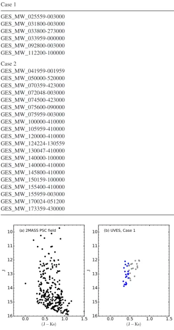
The target selection box for UVES was defined using the 2MASS Point Source Catalog (2MASS PSC) photometry (Skrutskie et al.
2006). VISTA VHS photometry suffers saturation in the relevant magnitude range, while 2MASS delivers better photometry.
Table 4. UVES Milky Way fields withJ=11 mag selection limit.
Figure 8. Colour–magnitude diagrams with 2MASS PSC photometry. (a) CMD of the field GES_MW_142000-050000 centred at Galactic longitude l=339.◦9 and latitudeb=51.◦4, and FoV=35 arcmin in diameter. (b) UVES target selection based on Case 1. Blue circles – selection of targets in the blue box, and grey stars – extra targets, respectively.
the brightest cut onJ2MASSof 11 instead of 12 mag and these are listed in Table4. The target selection maximum magnitude range for UVES inJ2MASSis 2.0 mag within the narrow range of (J−KS). Figs8and9show the UVES target selection for two Milky Way fields for Cases 1 and 2, respectively.
6 F I N A L TA R G E T S E L E C T I O N : A L L O C AT I N G T H E F I B R E S
The selected potential target lists were generated using the method-ology presented in Sections 3.1 and 3.2. Thereafter, the observing team generated the final target allocation catalogue that was used for the actual observations at the VLT.
Figure 9. Colour–magnitude diagrams with 2MASS PSC photometry. (a) CMD of the field GES_MW_201959-470000 centred at Galactic longitude l=352◦.7 and latitudeb= −34◦.2, and FoV=35 arcmin in diameter. (b) UVES target selection based on Case 2 showing the selected targets in the blue.
The target list has a larger FoV (35 arcmin) in diameter than the FoV for FLAMES and hence has a larger number of targets per field than can be allocated on FLAMES (see Fig.1and red filled circles versus blue squares in Fig.10). This large size of the potential target list is motivated by the fact that for each observing block a guide star must also be allocated and that it is of interest to allocate as many fibres as possible. To allow for some flexibility of the centre of the final field the list of potential targets hence covers a larger area on the sky. The centres of the allocated target lists are close to the original field centres.
The observing team uses the Fibre Positioner Observation Sup-port Software (FPOSS; see the user manual3for more details), which is the fibre configuration program for the preparation of FLAMES observations.FPOSStakes as input a file containing a list of target objects and generates a configuration in which as many fibres as possible are allocated to targets, allowing for the various instru-mental constraints and any specified target priorities. It produces a file containing a list of allocations of fibres to targets, the so-called target setup file.
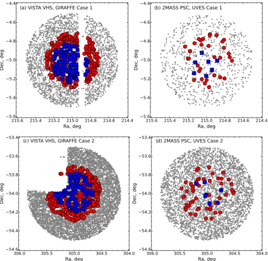
The final Gaia-ESO Survey target selection function depends on the allocated and observed targets. An illustration of two fields from Case 1 and Case 2 is shown in Fig.10. Here, targets are shown spatially distributed on the sky within the three different field-of-view introduced in Fig. 1 and discussed earlier in this section. Grey dots show targets distributed in a 1 deg2FoV in diameter; red filled circles show targets within 35 arcmin FoV in diameter (the one used to make the allocations); and blue filled squares show allocated FLAMES targets, with 25 arcmin FoV in diameter for two different Milky Way fields centred at Galactic longitudel=339◦.9, latitudeb=51◦.39 andl=344◦.3,b= −34◦.5, respectively.
There are several interesting points to extract from this illus-tration. First, it can be seen by visual inspection that Figs10(a) and (c) show the incompleteness of the VISTA VHS catalogue at the time when the catalogue was used for GIRAFFE target selec-tion. Figs10(a) and (b) show Case 1 for GIRAFFE and UVES, respectively. In this example, a total of 111 targets (including 33 second priority targets) were allocated on FLAMES/GIRAFFE for the Milky Way field centred at Galactic longitudel=339◦.9 and latitudeb=51◦.39 (Fig.10a). The total number of allocated targets
3https://www.eso.org/sci/facilities/paranal/instruments/flames/doc/
Figure 10. Spatial target distribution on the sky. (a) and (b) Milky Way field GES_MW_142000-050000 centred at Galacticl=339◦.9 andb=51◦.39, and selected based on Case 1 and VISTA VHS, 2MASS photometry; and (c), (d) field GES_MW_201959-540000 centred at Galacticl=344◦.3 andb= −34.◦5, and selected based on Case 2, respectively. Grey dots – targets distributed in a 1 deg2FoV in diameter; red filled circles – targets within 35 arcmin FoV in diameter; blue filled squares – allocated FLAMES targets, with 25 arcmin FoV in diameter.
on FLAMES/UVES for the same field is seven (including three as second priority targets) (Fig10b). The rest of the fibres were sky fibres. Figs10(c) and (d) show an example of Case 2, for the field GES_MW_201959-540000 centred at Galacticl=344◦.3 andb= −34◦.5. A total of 104 fibres were allocated (with∼80 per cent from the blue box and∼20 per cent from the red box) for GIRAFFE and seven for UVES.
7 W E I G H T S
7.1 Targeted and allocated weights
The selection function presented here consists of two steps. The first step is where potential targets are selected for GIRAFFE and UVES. The second step, final target allocation, is generating the actual list for observation.
Here, we present the weights per field calculated after the target selection and allocation. These weights can be used to better under-stand theGaia-ESO Survey results and correct them for selection bias.
The general weight per field for the primary target selection is
WT,F= NT
NF, (8)
where NT is the number of targeted objects in the field within 35 arcmin FoV in diameter.NFis the number of objects in the field within a 1 deg FoV in diameter (see Fig.1).WT, Fis the weight of targeted objects versus objects in the 1 deg FoV in diameter field. To countNFfor GIRAFFE targets we used the latest version of the VISTA VHS catalogue (version 2015-04). We use the same VHS quality flags as in Table3except for the flag (iv) (VHS not on the badCCD).
The general weight per field for the final target selection is
WA,T= NA
NT, (9)
whereNA is the number of allocated objects in the field within the FLAMES 25 arcmin FoV in diameter.WA, Tis the weight of allocated objects versus targeted for a given Milky Way field.
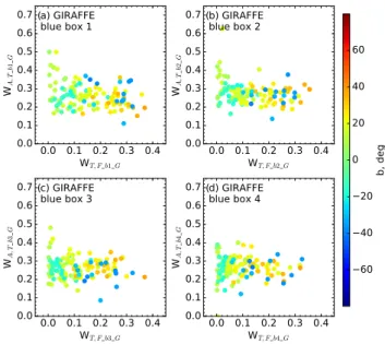
Since the target selection function is complex, we calculated weights for all the CMD colour boxes separately (i.e. blue, red and extra) (Figs11 and12). For Case 2, we calculated the blue box weights perJ1–4magnitude bins in each field within the given FoV (Figs13 and14). Hereafter,J1–4 = (Jmax − Jmin)/4, whereJ1 is the bright limit, andJ4is the faint limit of theJmagnitude. All calculated CMD weights per field are listed in Table1.
Figure 11. Weights of each field for targeted stars versus stars in the field within a 1 deg FoV in diameter compared with weights for allocated versus targeted stars in (a) blue, (b) red and (c) extra boxes for GIRAFFE. The colour coding indicates Galactic latitude in degrees.
Figure 12. Weights of each field for targeted stars versus stars in the field within a 1 deg FoV in diameter compared with weights for allocated versus targeted stars in (a) blue and (b) extra boxes for UVES. The colour coding indicates Galactic latitude in degrees.
Figure 13. Weights of each field for targeted stars versus stars in the field within a 1 deg FoV in diameter compared with weights for allocated versus targeted stars in blue box for GIRAFFE. (a)–(d) show weights inJ1–4 mag-nitude bins in fields within given FoV. The colour coding indicates Galactic latitude in degrees.
Fig.15). Case 1 Milky Way fields have higherWT, Fvalues than the Case 2 fields, but at the same time, theWT, Fvalues are different for each individual field within the two cases.
In order to use Milky Way field stars for a specific science ques-tion, we must understand how the spectroscopic sample is drawn from the underlying population. As can be seen from Fig.15, the
Figure 14. Weights of each field for targeted stars versus stars in the field within a 1 deg FoV in diameter compared with weights for allocated versus targeted stars in blue box for UVES. (a)–(d) show weights inJ1–4magnitude bins in fields within given FoV. The colour coding indicates Galactic latitude in degrees.
completeness of theGaia-ESO Survey varies substantially between fields. For each field, we must therefore assess how representative the spectroscopic sample is of the underlying population. To correct for these types of biases the presented weights,WT, F;WA, T, should be used.
7.2 Using iDR4: stellar weights for the colour–magnitude diagram
Figure 15. The distribution, shown in Mollweide projection with the Galactic centre in the middle, of the observed Milky Way fields across the sky. (a) and (b) show fields selected within the red box based on Cases 1 and 2, respectively, and observed with GIRAFFE. The colour coding indicates the weightWT,F (equation 8).
Figure 16. Distribution of the Milky Way field stars observed in iDR4, GIRAFFE that did not receive recommended stellar parameters in the same data release. These are split into the blue (a) and red (b) boxes.
are more likely to fail, due to the lower S/N of the spectra obtained. This is shown clearly in Fig.16, where all stars observed in iDR4 that failed to result in stellar parameters are plotted on the colour– magnitude diagram. There are 3849 stars in the blue box without parameters (e.g.Teff, log(g), [Fe/H]), and 856 in the red box.
To correct for these biases, each star that has values for the recommended stellar parameters in iDR4 needs a second weighting. This will ensure that results from the data release can be properly interpreted in terms of the actual populations of the Milky Way.
7.2.1 The CMD grids
To calculate the weights for iDR4 stars, we divide the colour– magnitude diagram into a grid of bins. The bin size is sufficiently small to accurately reflect the local sampling around each observed star. An example field is shown in Figs17(a) and (b), and it can be seen that the grid is larger than the original selection box. We are using the latest VISTA VHS photometry to calculate these weights, however many of the fields were observed some time ago, and the selection was completed with an older version of the VISTA VHS catalogues. The magnitudes in the updated catalogues differ from the older catalogues by a very small amount, but these differences are enough to mean that some stars which previously fell inside the selection box now lie slightly outside. The larger grid allows us to include weights for those stars as well. The red box is divided into
bins of size 0.05 in (J−KS), and 0.5 inJ. The grid for the blue box was designed to overlap with the four magnitude boxes that were defined in Section 3.2.2 for Case 2 fields. Therefore the bins are 0.4375 long inJ(half the size of the magnitude boxesJ1–4), and again 0.05 wide in (J−KS).
A similar setup is used for the UVES blue box (see Fig.17c) as in the GIRAFFE blue box, with different sized magnitude bins again to match the boxes in Case 2 fields; the bins are 0.5 long inJ, and remain 0.05 wide in (J−KS). In order to cope with those fields which had a bright limit ofJ2MASS=11 rather thanJ2MASS=12, the grid has been extended, as shown in Fig.17(c).
7.2.2 Weights of successfully observed targets
The weight of a successfully observed target in each CMD bin is calculated as follows:
WObin,Fbin= NObin NFbin
, (10)
whereNObinis the number of successfully observed targets in that bin, andNFbinis the number of objects in the VISTA VHS or 2MASS photometry for that bin. It is important to note thatNObin is not the same asNAbin, that is, the number of allocated objects in the bin, becauseNObinonly counts those objects that were successfully observed and have parameters in iDR4. The weightsWObin,Fbin of successfully observed stars with GIRAFFE and UVES are listed in Tables5and6where ‘CNAME’ is aGaia-ESO surveys specific stellar ID. The weights have not been calculated for those stars which fell into the extra box in Case 1 fields and not for SDSS and SkyMapper targets. We decided not to compare the stars in the extra box with stars from other fields with Case 1 selection, because targets within the extra box were selected with right-edge extensions varying between the fields (see Fig.4).
8 A F I R S T L O O K AT iD R 4 S U C C E S S F U L LY A N A LY S E D DATA
Figure 17. The colour–magnitude diagrams of an example of Milky Way field (GES_MW_023959-560000) for both the blue (a) and red (b) boxes for GIRAFFE and (c) blue box for UVES. In (a) and (b) the background VISTA VHS and (c) 2MASS photometry (black points) and successfully observed targets (red and blue points) are shown. The red and blue solid lines outline the boxes used to select the targets, and the dashed lines show the grid of bins for weighting.
Table 5. CMD weights of successfully observed stars with GIRAFFE in iDR4. The full table is available online.
CNAME GES_FLD RA(deg) Dec(deg) W_O,F_G W_Total_G Box
00000301-5455591 GES_MW_000024-550000 0.0125 −54.9331 0.133 3333 0.017 3717 Blue
00000377-5506384 GES_MW_000024-550000 0.0157 −55.1107 0.200 0000 0.026 0576 Blue
00000395-5458308 GES_MW_000024-550000 0.0165 −54.9752 1.000 0000 0.130 2880 Blue
00000533-5459505 GES_MW_000024-550000 0.0222 −54.9974 0.250 0000 0.032 5720 Blue
00000648-5451013 GES_MW_000024-550000 0.0270 −54.8504 0.150 0000 0.019 5432 Blue
... ... ... ... ... ... ...
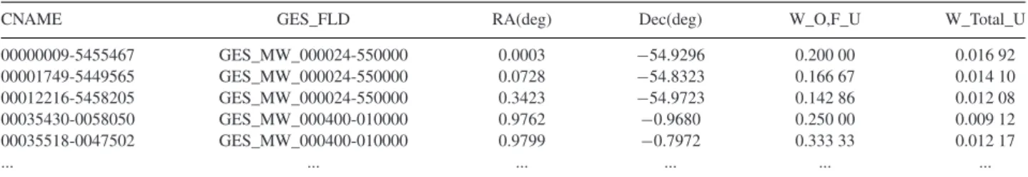
Table 6. CMD weights of successfully observed stars with UVES in iDR4. The full table is available online.
CNAME GES_FLD RA(deg) Dec(deg) W_O,F_U W_Total_U
00000009-5455467 GES_MW_000024-550000 0.0003 −54.9296 0.200 00 0.016 92
00001749-5449565 GES_MW_000024-550000 0.0728 −54.8323 0.166 67 0.014 10
00012216-5458205 GES_MW_000024-550000 0.3423 −54.9723 0.142 86 0.012 08
00035430-0058050 GES_MW_000400-010000 0.9762 −0.9680 0.250 00 0.009 12
00035518-0047502 GES_MW_000400-010000 0.9799 −0.7972 0.333 33 0.012 17
... ... ... ... ... ...
Therefore we looked at theGaia-ESO Survey iDR4 data. The in-ternal DR4 is a full release. All observations from the beginning of the survey until 2014 July are included.
Not surprisingly, the S/N varies withJmagnitude. We made a potential quality cut on S/N ratio of the spectra. Inspecting the spec-troscopic results (e.g.Teff, [Fe/H]) we chose to cut the spectroscopic sample at a median S/N>20. This cut might be different if one wants to consider other spectroscopic results e.g. alpha abundance. Fig.18shows the relation between the potential photometric sample (black contours), the spectroscopic sample (green contours), and af-ter the quality cut on S/N (yellow contours) for the Milky Way field GIRAFFE sample. In our case, while the sampling in colour is close to unbiased, the sampling inJis strongly biased against faint targets because of the signal-to-noise cut (S/N>20). Similar trends are seen in the SEGUE G-dwarf sample analysed by Bovy et al. (2012). Introducing this quality cut we lose about one magnitude in depth for targets within the blue box, while the sampling in the red box is not that affected (see Fig.18).
Here we provide a simple example of how one can use the pre-sented weights. We select Milky Way field stars observed with GI-RAFFE from iDR4 data within blue and red boxes and with [Fe/H] <0.50 (i.e. the more metal-rich targets are very uncommon). Here we chose to look at GIRAFFE targets only and show an application of the presented weights but in principal the calculated weights can be applied to UVES targets as well. These weights can be applied on top of the selection function weights described in Section 7.1, by multiplying them together as follows:
WTotal=WA,T×WT,F×WObin,Fbin, (11)
whereWTotalis the total weight. The total weightWTotalof a success-fully observed star with GIRAFFE and UVES are listed in Tables5
and6.
Figure 18. Distribution of the photometric sample of theGaia-ESO Survey Milky Way fields in blue (a, c) and red (b, d) boxes (linear density grey-scale, black contours). The observed spectroscopic sample of theGaia-ESO Survey iDR4 is shown as green contours; yellow contours show the spectroscopic sample with determined effective temperature and the signal-to-noise ratio cut of S/N>20. The black, green and yellow contours contain 68, 95 and 99 per cent of the distribution of Case 1 and Case 2 Milky Way field stars. On thex-axis we show the dereddened (J−Ks)0colour, whereas on they-axis we show the observedJ magnitude.
is to use the blue box weight for those stars (607 stars in iDR4) when combining blue and red box data.
We can therefore, when trying to accurately sample the Milky Way disc, characterize the importance of an observed star in iDR4 by giving it a weight. In order to make a correction for each success-fully observed star in our sample, we give the total weightWTotal as 1/WTotal. Here we effectively tell how frequent a successfully observed stars is with a givenJand (J−Ks) within a given Milky Way field in a given FoV. In this example we chose to remove stars where 1/WTotal> 100 000, because in this case the weight is too large to be meaningful, and the star is not representative of the sam-ple. Essentially, this cut removes 1.2 per cent of blue box targets and 0.2 per cent of red box targets.
In Fig.19, we show an application of the weights presented in this paper. We see that the metallicity distribution of stars observed in the
Gaia-ESO Survey iDR4 with GIRAFFE in the blue and red boxes (blue and red line) are different from the weighted distributions (black dashed line) when all Milky Way fields are analysed together. We find that for the red box the observed distribution is the same as the underlying distribution, but this is not the case for the blue box, as seen by comparing their respective cumulative distributions, corrected versus uncorrected (see Figs19c and d). The total weight,
WTotal, normalizes between the different lines of sight; while each observed Milky Way field has almost the same number of spectra, but not the same number of successfully analysed stars and different number of photometric objects varying per line of sight due to the nature of the Galaxy. This is a simple example to highlight the necessity of including such information in studies of the stellar populations in the Milky Way. There are other ways how one can apply presented weights (i.e. taking into account the [Fe/H] errors, looking at different lines of site or combining blue and red box targets together).
The presented field CMD weights (WA,T,WT,F) and the weights of successfully observed targets (WObin,Fbin) can be used differently than in the previous example. For example, looking at the radial and/or vertical metallicity distribution the weights can be used to limit the data to only those stars that most represent the underlying population. In this case, we do not want stars with very smallWTotal to contribute to the analysis, since they do not provide enough information about the actual underlying population. A simple way of studying the Milky Way’s radial metallicity gradient is to bin the data in Galactocentric radial distanceRand compute the mean metallicity in each bin as a running average. However, instead of computing a straight mean, we can perform a weighted average, in which each star is weighted byWTotal. This will then bias the
mean metallicity towards those stars with the highestWTotal. The results can then be compared with those for the standard mean to understand possible biases in the data.
9 C O N C L U S I O N S A N D F U T U R E P R O S P E C T S
We have discussed the details of the selection function for the Milky Way field stars observed in theGaia-ESO Survey. The weights pre-sented here are based on targets selected from the beginning of the survey up to the end of 2015 June. To characterize the major components of the Galaxy, and to understand these components in the context of the Milky Way’s formation and evolution history, the survey selection function is designed to target stars as homoge-neously as possible throughout the Milky Way. The target selection is based on stellar magnitudes and colours, using photometry from the VHS (McMahon et al.2013) and 2MASS (Skrutskie et al.2006). Also we present the basic and actual target selection schemes for the Milky Way field stars observed with FLAMES/GIRAFFE and FLAMES/UVES.
The actual target selection scheme is divided into two cases. In Case 1 the target selection algorithm, in addition to the two main selection CMD boxes (i.e. blue, red), extends the colour limits to select second priority targets (i.e. for those Milky Way fields where the density of stars is not enough to fill the FLAMES fibres). Case 2 is used to select targets near the Galactic plane. In this case, the target selection algorithm is configured to select the same number of targets per magnitude bin (i.e. not to have a bias towards very faint stars).
From the beginning of the survey on 2011 December 31 until 2015 June, a total of 330 Milky Way fields have been targeted and allocated on FLAMES. 202 Milky Way fields were selected using Case 1 and 118 using Case 2, which were then allocated on FLAMES/GIRAFFE. For UVES, 164 and 166 Milky Way fields were used in Case 1 and Case 2, respectively. In addition, a sample of Milky Way fields were selected to target rare but astrophysically important stellar populations (e.g. metal-poor stars, K giants), where Milky Way field targets were selected using the SDSS photometry (Ahn et al.2012) and SkyMapper photometry (Keller et al.2007), for allocation on FLAMES/GIRAFFE and FLAMES/UVES.
Figure 19. The metallicity distribution of all Milky Way field stars observed with GIRAFFE in theGaia-ESO Survey iDR4. (a, c) and (b, d) show metallicity distribution of stars within blue and red boxes, respectively. The blue and red lines show the observed metallicity; the black dashed lines show weighted metallicity distributions. Only stars with [Fe/H]<0.50 are included.
and allocation. These weights can be used to better understand the
Gaia-ESO Survey results and correct selection biases for the proper interpretation of the data in terms of our understanding of the Milky Way as a galaxy.
We are continuing our work on weights application for theGaia -ESO Survey Milky Way field GIRAFFE data and the results will be presented in a forthcoming paper. Here we presented weights per field for targeted and allocated Milky Way stars observed up to end of 2015 June and weights of successfully observed iDR4 stars 15 154 for GIRAFFE and 1367 for UVES and we plan to continue our work on the target selection function for Milky Way stars when the next data set is available.
AC K N OW L E D G E M E N T S
ES, LH, SF, GRR and TB acknowledge support from the project grant ‘The New Milky Way’ from the Knut and Alice Wallenberg Foundation. RS acknowledges support from NCN/Poland through grant 2014/15/B/ST9/03981. AJK acknowledges support by the Swedish National Space Board. We thank the anonymous referee for her/his constructive comments, which have improved the clarity of the paper. Based on data products from observations made with ESO Telescopes at the La Silla Paranal Observatory under programme ID 188.B-3002. These data products have been processed by the CASU at the Institute of Astronomy, University of Cambridge, and by the FLAMES/UVES reduction team at INAF/Osservatorio As-trofisico di Arcetri. These data have been obtained from theGaia -ESO Survey Data Archive, prepared and hosted by the Wide Field Astronomy Unit, Institute for Astronomy, University of Edinburgh, which is funded by the UK Science and Technology Facilities Coun-cil. This work was partly supported by the European Union FP7
programme through ERC grant number 320360 and by the Lev-erhulme Trust through grant RPG-2012-541. We acknowledge the support from INAF and Ministero dell’ Istruzione, dell’ Universit`a’ e della Ricerca (MIUR) in the form of the grant ‘Premiale VLT 2012’. The results presented here benefit from discussions held during theGaia-ESO workshops and conferences supported by the ESF (European Science Foundation) through the GREAT Research Network Programme. Based on observations obtained as part of the VHS, ESO Program, 179.A-2010 (PI: McMahon). Funding for SDSS-III has been provided by the Alfred P. Sloan Foundation, the Participating Institutions, the National Science Foundation, and the US Department of Energy Office of Science. The SDSS-III website ishttp://www.sdss3.org/.
R E F E R E N C E S
Ahn C. P. et al., 2012, ApJS, 203, 21 Bergemann M. et al., 2014, A&A, 565, A89
Bland-Hawthorn J., Gerhard O., 2016, preprint (arXiv:1602.07702) Bovy J., Rix H.-W., Liu C., Hogg D. W., Beers T. C., Lee Y. S., 2012, ApJ,
753, 148
Cheng J. Y. et al., 2012, ApJ, 746, 149
Cirasuolo M. et al., 2012, in McLean I. S., Ramsay S K., Takami H., eds, Proc. SPIE Conf. Ser. Vol. 8446, Ground-based and Airborne Instru-mentation for Astronomy IV. SPIE, Bellingham, p. 84460S
Dalton G. et al., 2012, in McLean I. S., Ramsay S K., Takami H., eds, Proc. SPIE Conf. Ser. Vol. 8446, Ground-based and Airborne Instrumentation for Astronomy IV. SPIE, Bellingham, p. 84460P
Dekker H., D’Odorico S., Kaufer A., Delabre B., Kotzlowski H., 2000, in Iye M., Moorwood A. F., eds, Proc. SPIE Conf. Ser. Vol. 4008, Optical and IR Telescope Instrumentation and Detectors. SPIE, Bellingham, p. 534
Deng L.-C. et al., 2012, Res. Astron. Astrophys., 12, 735 Donati P. et al., 2014, A&A, 561, A94
Feltzing S., Chiba M., 2013, New Astron. Rev., 57, 80 Francis C., 2013, MNRAS, 436, 1343
Freeman K., Bland-Hawthorn J., 2002, ARA&A, 40, 487 Gilmore G. et al., 2012, The Messenger, 147, 25 Howes L. M. et al., 2014, MNRAS, 445, 4241 Jackson-Jones R. et al., 2014, A&A, 571, L5 Keller S. C. et al., 2007, PASA, 24, 1 Koposov S. E. et al., 2015, ApJ, 811, 62 Kordopatis G. et al., 2015, A&A, 582, A122 Liu C., van de Ven G., 2012, MNRAS, 425, 2144
McMahon R. G., Banerji M., Gonzalez E., Koposov S. E., Bejar V. J., Lodieu N., Rebolo R., VHS Collaboration, 2013, The Messenger, 154, 35 Magrini L. et al., 2015, A&A, 580, A85
Majewski S. R. et al., 2015, preprint (arXiv:1509.05420) Mikolaitis ˇS. et al., 2014, A&A, 572, A33
Nidever D. L. et al., 2014, ApJ, 796, 38
Nishiyama S., Tamura M., Hatano H., Kato D., Tanab´e T., Sugitani K., Nagata T., 2009, ApJ, 696, 1407
Pasquini L. et al., 2002, The Messenger, 110, 1 Perryman M. A. C. et al., 2001, A&A, 369, 339
Randich S., Gilmore G., Gaia-ESO Consortium, 2013, The Messenger, 154, 47
Recio-Blanco A. et al., 2014, A&A, 567, A5 Rieke G. H., Lebofsky M. J., 1985, ApJ, 288, 618 Ruchti G. R. et al., 2015, MNRAS, 450, 2874 San Roman I. et al., 2015, A&A, 579, A6
Schlegel D. J., Finkbeiner D. P., Davis M., 1998, ApJ, 500, 525 Schlesinger K. J. et al., 2012, ApJ, 761, 160
Skrutskie M. F. et al., 2006, AJ, 131, 1163 Steinmetz M. et al., 2006, AJ, 132, 1645 Tautvaiˇsien˙e G. et al., 2015, A&A, 573, A55 Yanny B. et al., 2009, AJ, 137, 4377
S U P P O RT I N G I N F O R M AT I O N
Additional Supporting Information may be found in the online ver-sion of this article:
Table 1.Main parameters and weights of the targeted and allocated Milky Way fields.
Table 5. CMD weights of successfully observed stars with GI-RAFFE in iDR4.
Table 6.CMD weights of successfully observed stars with UVES in iDR4 (http://www.mnras.oxfordjournals.org/lookup/suppl/doi: 10.1093/mnras/stw1011/-/DC1).
Please note: Oxford University Press is not responsible for the content or functionality of any supporting materials supplied by the authors. Any queries (other than missing material) should be directed to the corresponding author for the article.
A P P E N D I X A : C A L C U L AT E D C M D W E I G H T S
For each Milky Way field observed from the beginning of theGaia -ESO Survey until 2015 June, we calculated CMD weights per field
WT, FandWA, T to correct for potential biases. Those Milky Way fields and associated field weights are in Table1and the meanings of acronyms used are in TableA1. Full version of Table1is available online.
A P P E N D I X B : A D D I T I O N A L F I E L D S
A subset of fields were allocated to specially selected candidate targets belonging to rare but astrophysically important stellar popu-lations, such as metal-poor stars or K giants. Those additional fields inGaia-ESO survey are labelled as Milky Way fields. The target selection for those additional fields is different from the Milky Way fields presented in this paper. The additional fields were created with the target selection based on SkyMapper photometry (Keller et al.2007), SDSS photometry (Ahn et al.2012), VISTA VHS pho-tometry and 2MASS phopho-tometry (see location of the fields on the sky in Fig.5a). In the following sections we present those different selections.
B1 Milky way fields selected to study the outer Galactic disc
Three additional Milky Way fields were selected using SDSS pho-tometry in order to study the outer disc of the Galaxy. GIRAFFE fibres were allocated to candidate K giants, which probe the far outer disc, warp and flare.
The SDSS catalogue flags adopted to select these Milky Way field targets are listed in Table3. The target selection of the additional fields in the blue and extra boxes with SDSS photometry is as follows:
HereSDSSis the right-edge extension of the blue box.SDSSand the Milky Way field names selected with the SDSS photometry are listed in TableB1. The selection of UVES targets in the same Milky Way fields is based on 2MASS photometry as described in Section 5.
B2 Milky Way fields with metal-poor stars in the halo
B2.1 Milky Way fields with the target selection based on SkyMapper photometry and 2MASS photometry
Seven additional Milky Way fields were selected using SkyMapper photometry in order to study the metal-poor stars in the halo.
All GIRAFFE targets were selected from the SkyMapper photom-etry. For the same Milky Way fields only one UVES fibre per field was devoted to observe a metal-poor star selected using SkyMap-per photometry. The remaining UVES targets were selected using 2MASS photometry.
Milky Way field names for which SkyMapper photometry was used to select the targets to be observe with GIRAFFE and one target to be observed with UVES are listed in TableB2.
B2.2 Milky Way fields with the target selection based on SkyMapper photometry, 2MASS photometry and VISTA VHS photometry
Table A1. The meanings of acronyms used in Table1.
Col_No Acronym Meaning
(1) GES_FLD GES Milky Way field name from CASU.
(2) RA RA [h:m:s] of GES Milky Way field centre.
(3) Dec Dec [d:m:s] of GES Milky Way field centre.
(4) E(B−V) The Galactic dust extinction median value measured from the Schlegel, Finkbeiner & Davis (1998) maps. (5) G The right-edge limit of second priority targets for GIRAFFE.
(6) U The right-edge limit of second priority targets for UVES.
(7) W_T,F_b_G The weight of blue box for GIRAFFE, where targeted star counts are versus star counts in 1◦FoV. (8) W_T,F_b1_G The weight of blue box withJ1 for GIRAFFE, where targeted star counts are versus star counts in 1◦FoV. (9) W_T,F_b2_G The weight of blue box withJ2 for GIRAFFE, where targeted star counts are versus star counts in 1◦FoV. (10) W_T,F_b3_G The weight of blue box withJ3 for GIRAFFE, where targeted star counts are versus star counts in 1◦FoV. (11) W_T,F_b4_G The weight of blue box withJ4 for GIRAFFE, where targeted star counts are versus star counts in 1◦FoV. (12) W_T,F_r_G The weight of red box for GIRAFFE, where targeted star counts are versus star counts in 1◦FoV. (13) W_T,F_e_G The weight of extra box for GIRAFFE, where targeted star counts are versus star counts in 1◦FoV. (14) W_A,T_b_G The weight of blue box for GIRAFFE, where allocated star counts are versus targeted star counts. (15) W_A,T_b1_G The weight of blue box withJ1 for GIRAFFE, where allocated star counts are versus targeted star counts. (16) W_A,T_b2_G The weight of blue box withJ2 for GIRAFFE, where allocated star counts are versus targeted star counts. (17) W_A,T_b3_G The weight of blue box withJ3 for GIRAFFE, where allocated star counts are versus targeted star counts. (18) W_A,T_b4_G The weight of blue box withJ4 for GIRAFFE, where allocated star counts are versus targeted star counts. (19) W_A,T_r_G The weight of red box for GIRAFFE, where allocated star counts are versus targeted star counts. (20) W_A,T_e_G The weight of extra box for GIRAFFE, where allocated star counts are versus targeted star counts. (21) W_T,F_b_U The weight of blue box for UVES, where targeted star counts are versus star counts in 1◦FoV. (22) W_T,F_b1_U The weight of blue box withJ1 for UVES, where targeted star counts are versus star counts in 1◦FoV. (23) W_T,F_b2_U The weight of blue box withJ2 for UVES, where targeted star counts are versus star counts in 1◦FoV. (24) W_T,F_b3_U The weight of blue box withJ3 for UVES, where targeted star counts are versus star counts in 1◦FoV. (25) W_T,F_b4_U The weight of blue box withJ4 for UVES, where targeted star counts are versus star counts in 1◦FoV. (26) W_T,F_e_U The weight of extra box for UVES, where targeted star counts are versus star counts in 1◦FoV. (27) W_A,T_b_U The weight of blue box for UVES, where allocated star counts are versus targeted star counts. (28) W_A,T_b1_U The weight of blue box withJ1 for UVES, where allocated star counts are versus targeted star counts. (29) W_A,T_b2_U The weight of blue box withJ2 for UVES, where allocated star counts are versus targeted star counts. (30) W_A,T_b3_U The weight of blue box withJ3 for UVES, where allocated star counts are versus targeted star counts. (31) W_A,T_b4_U The weight of blue box withJ4 for UVES, where allocated star counts are versus targeted star counts. (32) W_A,T_e_U The weight of extra box for UVES, where allocated star counts are versus targeted star counts. (33) Blue(per cent) The approximate fraction of targets in the blue versus the red box (per cent).
Table B1. Milky Way fieldsa for which SDSS photometry was used to
select the targets to be observe with GIRAFFE (see Appendix B1).
Milky Way fields SDSS
GES_MW_082312-052959 –
GES_MW_083959-003000 0.41
GES_MW_095600-003000 –
Note.aFor UVES targets the selection is based on 2MASS photometry.
Table B2. Milky Way fields for which SkyMapper photometry was used to select the targets to be observe with GIRAFFE and one target to be observed with UVESa(see Appendix B2.1).
Milky Way fields GES_MW_094753-102657 GES_MW_100913-412801 GES_MW_101428-405235 GES_MW_105731-124726 GES_MW_105808-154324 GES_MW_110053-132816 GES_MW_131359-460007
Note. aThe remaining UVES targets are selected based on 2MASS
photometry.
Table B3. Milky Way fields with the target selection based on SkyMappera
photometry, 2MASSb photometry and VISTA VHSc photometry (see
Appendix B2.2). Milky Way fields GES_MW_125609-451238 GES_MW_133026-434759 GES_MW_142145-440827 GES_MW_144113-400831 GES_MW_212402-431239 GES_MW_212731-542154 GES_MW_221259-455029 GES_MW_221818-582824 GES_MW_225008-554935 GES_MW_225108-524744 GES_MW_234854-560538
Notes.aOnly one SkyMapper target per field was observed by UVES. bThe remaining UVES targets were selected based on 2MASS photometry. cFor GIRAFFE targets the selection is based on VISTA VHS photometry.
photometry was dedicated to study the most interesting metal-poor star in the halo. The remaining UVES targets were selected using 2MASS photometry.
For the GIRAFFE targets in the same Milky Way fields the selec-tion is based on VISTA VHS photometry as described in Secselec-tion 4.