DOI:10.1051/0004-6361/201730442 c
ESO 2017
Astronomy
&
Astrophysics
The
Gaia
-ESO Survey: double-, triple-, and quadruple-line
spectroscopic binary candidates
?
T. Merle
1, S. Van Eck
1, A. Jorissen
1, M. Van der Swaelmen
1, T. Masseron
2, T. Zwitter
3, D. Hatzidimitriou
4,5,
A. Klutsch
6, D. Pourbaix
1, R. Blomme
7, C. C. Worley
2, G. Sacco
8, J. Lewis
2, C. Abia
9, G. Traven
3, R. Sordo
10,
A. Bragaglia
11, R. Smiljanic
12, E. Pancino
8,21, F. Damiani
13, A. Hourihane
2, G. Gilmore
2, S. Randich
8, S. Koposov
2,
A. Casey
2, L. Morbidelli
8, E. Franciosini
8, L. Magrini
8, P. Jofre
2,22, M. T. Costado
14, R. D. Je
ff
ries
15,
M. Bergemann
16, A. C. Lanzafame
6,17, A. Bayo
18, G. Carraro
19, E. Flaccomio
13, L. Monaco
20, and S. Zaggia
10(Affiliations can be found after the references)
Received 16 January 2017/Accepted 5 July 2017
ABSTRACT
Context.TheGaia-ESO Survey (GES) is a large spectroscopic survey that provides a unique opportunity to study the distribution of spectroscopic multiple systems among different populations of the Galaxy.
Aims.Our aim is to detect binarity/multiplicity for stars targeted by the GES from the analysis of the cross-correlation functions (CCFs) of the GES spectra with spectral templates.
Methods.We developed a method based on the computation of the CCF successive derivatives to detect multiple peaks and determine their radial velocities, even when the peaks are strongly blended. The parameters of the detection of extrema (
doe
) code have been optimized for each GES GIRAFFE and UVES setup to maximize detection. Thedoe
code therefore allows to automatically detect multiple line spectroscopic binaries (SBn,n≥2).Results.We apply this method on the fourth GES internal data release and detect 354 SBncandidates (342 SB2, 11 SB3, and even one SB4), including only nine SBs known in the literature. This implies that about 98% of these SBncandidates are new because of their faint visual magnitude that can reachV=19. Visual inspection of the SBncandidate spectra reveals that the most probable candidates have indeed a composite spectrum. Among the SB2 candidates, an orbital solution could be computed for two previously unknown binaries: CNAME 06404608+0949173 (known as V642 Mon) in NGC 2264 and CNAME 19013257-0027338 in Berkeley 81 (Be 81). A detailed analysis of the unique SB4 (four peaks in the CCF) reveals that CNAME 08414659-5303449 (HD 74438) in the open cluster IC 2391 is a physically bound stellar quadruple system. The SB candidates belonging to stellar clusters are reviewed in detail to discard false detections. We suggest that atmospheric parameters should not be used for these system components; SB-specific pipelines should be used instead.
Conclusions.Our implementation of an automatic detection of spectroscopic binaries within the GES has allowed the efficient discovery of many new multiple systems. With the detection of the SB1 candidates that will be the subject of a forthcoming paper, the study of the statistical and physical properties of the spectroscopic multiple systems will soon be possible for the entire GES sample.
Key words. binaries: spectroscopic – techniques: radial velocities – methods: data analysis – open clusters and associations: general – globular clusters: general
1. Introduction
Binary stars play a fundamental role in astrophysics since they allow direct measurements of masses, radii, and luminosities that put constraints on stellar physics, Galactic archaeology, high-energy physics, etc. Binary systems are found at all evolutionary stages, and after strong interaction, some may end up as double degenerate systems or merged compact objects.
Spectroscopic binaries (SBs) exist in different flavours. On the one hand, SB1 (SBs with one observable spectrum) can only be detected from the Doppler shift of the stellar spec-tral lines. On the other hand, SBn (n ≥ 2) are characterized
?
Based on data products from observations made with ESO Tele-scopes at the La Silla Paranal Observatory under programme ID 188.B-3002. These data products have been processed by the Cambridge Astronomy Survey Unit (CASU) at the Institute of Astronomy, Uni-versity of Cambridge, and by the FLAMES/UVES reduction team at INAF/Osservatorio Astrofisico di Arcetri. These data have been ob-tained from theGaia-ESO Survey Data Archive, prepared and hosted by the Wide Field Astronomy Unit, Institute for Astronomy, Univer-sity of Edinburgh, which is funded by the UK Science and Technology Facilities Council.
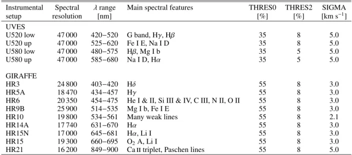
Table 1.Setups used in GES and the associated estimated best parameters of the
doe
code.Instrumental Spectral λrange Main spectral features THRES0 THRES2 SIGMA
setup resolution [nm] [%] [%] [km s−1]
UVES
U520 low 47 000 420−520 G band, Hγ, Hβ 35 8 5.0
U520 up 47 000 525−620 Fe I E, Na I D 35 8 5.0
U580 low 47 000 480−575 Hβ, Mg I b 35 5 5.0
U580 up 47 000 585−680 Na I D, Hα 35 5 5.0
GIRAFFE
HR3 24 800 403−420 Hδ 55 8 3.0
HR5A 18 470 434−457 Hγ 55 8 3.0
HR6 20 350 454−475 He I & II, Si III & IV, C III, N II, O II 55 8 3.0
HR9B 25 900 514−535 Mg I b, Fe I E 55 8 3.0
HR10 19 800 534−561 Many weak lines 55 8 2.1
HR14A 17 740 631−670 Hα 55 8 3.0
HR15N 17 000 645−681 Hα, Li I 55 8 3.0
HR15 19 300 660−695 O2A, Li I 55 8 3.0
HR21 16 200 849−900 Ca
ii
triplet, Paschen lines 55 8 5.0investigations of binarity over a large sample of stars (see e.g. Gao et al. 2014;Troup et al. 2016;Fernandez et al. 2017). For instance, the RAVE survey led to the detection of 123 SB2 can-didates out of 26 000 objects (Matijeviˇc et al. 2010,2011). We refer the reader toDuchêne & Kraus(2013) for a recent review of the physical properties of multiplicity among stars and more specifically to Raghavan et al. (2010) for a complete volume-limited sample of solar-type stars in the solar neighbourhood (distances closer than 25 pc).
The Gaia-ESO Survey (GES) is an ongoing ground-based high-resolution spectroscopic survey of 105 stellar sources (Gilmore et al. 2012; Randich et al. 2013) covering the main stellar populations of the Galaxy (bulge, halo, thin and thick discs) as well as a large number of open clusters spanning large metallicity and age ranges. All evolutionary stages are encoun-tered within the GES, from pre-main sequence objects to red giants. It aims to complement the spectroscopy of the Gaia ESA space mission (Wilkinson et al. 2005). The GES uses the FLAMES multi-fibre back end at the high-resolution UVES (R∼ 50 000) and moderate-resolution GIRAFFE (R ∼20 000) spec-trographs. The visual magnitude of the faintest targets reaches V ∼ 20. The spectral coverage spans the optical wavelengths (from 4030 to 6950 Å) and the near-infrared around the Ca
ii
triplet and the Paschen lines (from 8490 to 8900 Å includ-ing the wavelength range of the Radial Velocity Spectrometer of the Gaia mission). The median signal-to-noise ratio (S/N) per pixel is similar for UVES and GIRAFFE single exposures (∼30), whereas the most frequent values are around 20 and 5, respectively.The motivation of the present work is to take advantage of a very large sample to automatically detect SBs with more than one visible component1that are not always detected by the GES single-star main analysis pipelines. Spectroscopic binaries may be a potential source of error when deriving atmospheric pa-rameters and detailed abundances. This project presents a new method to automatically identify the number of velocity com-ponents in each cross-correlation function (CCF) using their successive derivatives and the analysis of about 51 000 stars available within the GES internal data release 4 (iDR4). 1 Since SB1 systems require a special treatment by analysing temporal series, their analysis should await the completion of the observations.
In Sect. 2, we describe the iDR4 stellar observations, their associated CCFs, and the selection criteria applied to them. The method used to detect the velocity components in a CCF, its pa-rameters, and the formal uncertainty are presented in Sect.3. In Sect.4, the set of SBn (n ≥ 2) detected in iDR4 using this method is discussed, organized according to the stellar popula-tions they belong to.
2. Data selection
2.1. Observations and CCF computation
Our analysis was performed on the iDR4 consisting of∼260 000 single exposures (corresponding to ∼100 000 stacked spectra) of about 51 000 distinct stars observed with the FLAMES in-strument feeding the optical spectrographs GIRAFFE (with se-tups HR3, HR5A, HR6, HR9B, HR10, HR14A, HR15N, HR15, HR21) and UVES (with setups U520 and U580) covering the optical and near-IR wavelength ranges given in Table1.
The classical definition of a CCF function applied to the stel-lar spectra is
CCF(h)= Z +∞
−∞
50 0 50 100 150 200 0.2
0.4 0.6
0.8 v1 = 71.94 original
selection
50 0 50 100 150 200
1.8 0.9 0.0 0.9
1.81e 2 1st derivative
50 0 50 100 150 200
1.8 0.9 0.0 0.9 1.8 1e 3
w1 = 27.23 2nd derivative
50 0 50 100 150 200
v [km/s]
2 0
2 1e 4 3rd derivative
50 0 50 100 150 200
0.2 0.4 0.6
0.8 v1 = 71.79 original
selection
50 0 50 100 150 200
2 0 2 4 1e 2
1st derivative
50 0 50 100 150 200
4 2 0
21e 3w1 = 22.35 2nd derivative
50 0 50 100 150 200
v [km/s] 0.5
0.0 0.5
1e 3
3rd derivative
Fig. 1.Simulated CCF at limiting numerical resolution to test the computation of successive derivatives and the detection of the peak (left), and with a more realistic sampling (right). The spectrum used to simulate these CCFs has a radial velocity of 72.0 km s−1andS/N=5.
point of the CCF tail) and a full amplitude (maximum – min-imum). The constant velocity steps of GIRAFFE and UVES CCFs are 2.75 (mainly) and 0.50 km s−1(for a sampling of 401 and 4000 velocity points), respectively.
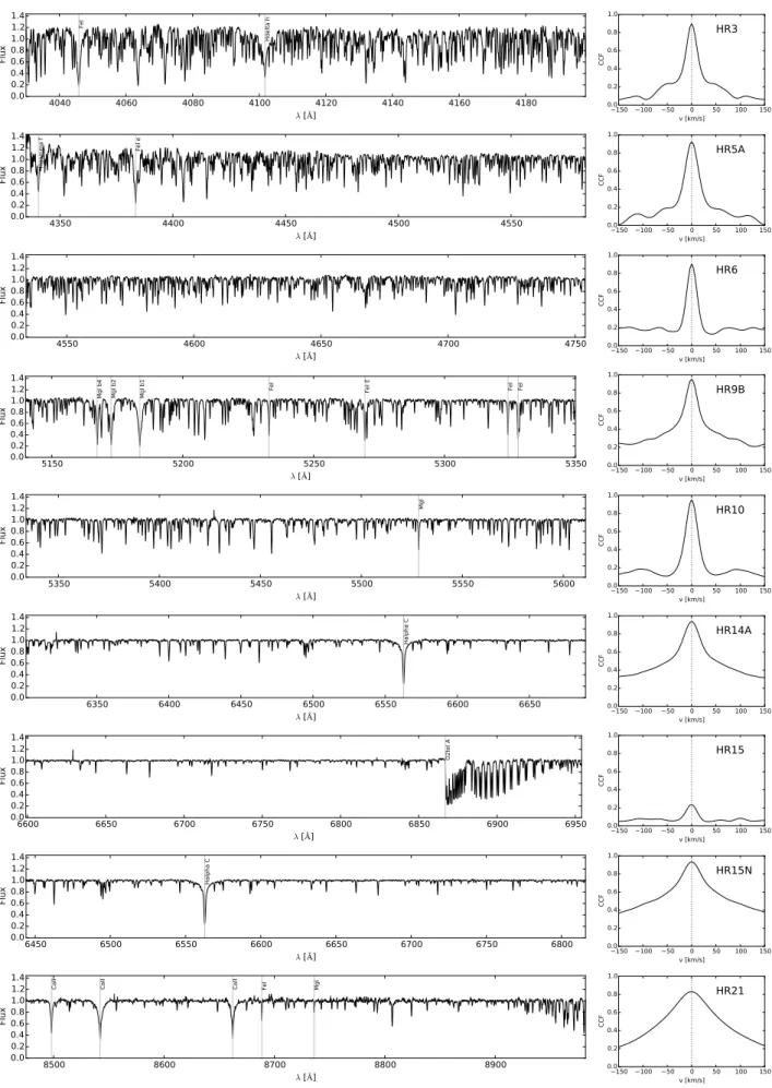
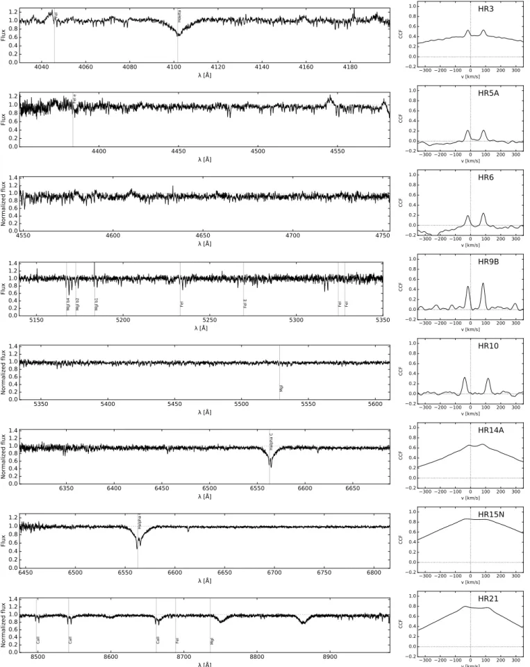
Examples of spectra and CCFs in the setups mentioned above are displayed in Figs.2and3. These figures are built from the solar and Aldebaran spectra. The CCFs are represented over the same velocity range to allow an easy comparison between the various setups. When a lot of weak absorption lines are present (as in setups HR6 and HR10), the CCF peak is narrow and well-defined with a width smaller than for setups with strong fea-tures like Hδ(HR3), Hγ(HR5A), the Mg b triplet (HR9B), Hα (HR14A and HR15N), and the Ca II triplet (HR21). For HR15, the presence of telluric lines from 685 nm onwards reduces the maximum amplitude of the CCF to a value as low as 0.25, even with a S/N higher than 1000.
For the UVES setups, Aldebaran (αTau, spectral type K5III) spectra and corresponding CCFs are presented in Fig. 3. Each setup is composed of two spectral chunks. In the present case, the lower chunk comes withS/N ≈70 and the upper one with S/N > 100. For the setup U520 low, the leftward CCF tail is negative, probably as a result of poor spectrum normalization due to the co-existence of many weak and strong lines. Since the wavelength range of the UVES setups is 2 or 3 times wider than those of GIRAFFE, the UVES setups are well suited to detecting SBncandidates.
The final GES spectrum of a given object is a stack of all individual exposures, wavelength calibrated, sky subtracted, and heliocentric radial velocity corrected. This could be a source of confusion in the case of composite spectra where the radial ve-locity of the different components changes between exposures. Moreover, a double-lined CCF coming from stacked spectra (and mimicking an SB2) can be the result of the SB1 combination taken at different epochs and stacked. To avoid this problem, we performed the binarity detection on the individual exposures (rather than on the stacked ones). This choice avoids spurious spectroscopic binary detection at the expense of using spectra with lower S/N, which will be shown not to be detrimental as long asS/N>5 (see Sect.3.4).
The number of individual observations per target is plotted in Fig.4. Most of the stars observed with GIRAFFE have 2 or 4 ob-servations because generally observed with HR10 and HR21 se-tups, whereas there are 4 or 8 observations in the case of UVES, due to the presence of two spectral chunks per setup. Moreover, the time span between consecutive observations is very often less than three days, as shown in Fig. 5. Benchmark stars (i.e. a sample of stars with well-determined parameters to be used as reference; seeHeiter et al. 2015a) are the most observed objects, some having more than 100 observations.
2.2. Data selection in iDR4
Our sample has been drawn from the individual spectra database of the GES iDR43, covering observations until June 2014, to which the following selection criteria were applied:
– S/N higher than 5;
– CCF maximum larger than 0.15;
– CCF minimum larger than−1;
– CCF full amplitude larger than 0.10;
– left CCF continuum −right CCF continuum smaller than 0.15.
These criteria were empirically determined thanks to a visual inspection of a representative sample of CCFs. We allow neg-ative values for the CCF minimum to keep CCFs computed on unperfectly normalized spectra (without allowing spectra with a completely incorrect normalization). Criteria on the S/N and on the CCF maximum are presented in Fig.6for setups HR10 and HR21 which contain the most numerous observations. This figure clearly shows the impact of the S/N of a spectrum on its associated CCF: the higher the S/N, the higher the CCF maxi-mum. For a given S/N, the interval spanned by the CCF maxi-mum is mainly due to spectrum – template mismatch. For HR10, the over-density located at 30 < S/N < 200 and CCF max< 0.15 is mainly due to NGC 6705 members. In HR21, the clump 3 GES public data releases may be found at https://www.
4040 4060 4080 4100 4120 4140 4160 4180
4350 4400 4450 4500 4550
λ [ ]
4550 4600 4650 4700 4750
λ [ ]
5150 5200 5250 5300 5350
λ [ ]
5350 5400 5450 5500 5550 5600
λ [ ]
6350 6400 6450 6500 6550 6600 6650
λ [ ]
6600 6650 6700 6750 6800 6850 6900 6950
λ [ ]
6450 6500 6550 6600 6650 6700 6750 6800
λ [ ]
8500 8600 8700 8800 8900
λ [ ]
4200 4400 4600 4800 5000 5200
5400 5600 5800 6000 6200
λ [ ]
4800 5000 5200 5400 5600 5800
λ [ ]
6000 6200 6400 6600 6800
λ [ ]
Fig. 3.Spectra of Aldebaran (αTau) by GES in UVES setups withS/N≈70 for the low spectral chunks andS/N>100 for the upper chunks.
1
Fig. 4.Number of stars observed as a function of the number of ob-servations per star. A tiny fraction, including benchmark stars, have a number of observations that can reach∼100.
located at 1000 <S/N <2000 and 0.80<CCF max<0.85 is due to repeated observations of the solar spectrum.
These criteria allow us to avoid detecting spurious (noise-induced) CCF peaks. Over the 260 000 individual science spec-tra (corresponding to the 100 000 stacked specspec-tra) within the iDR4, 9.3% have a S/N lower than 5, 1.0% have a null CCF (data processing issues), 7.8% have a CCF maximum lower than 0.15, 0.2% have a CCF minimum lower than −1.0, and 0.02% have a CCF full amplitude lower than 0.10. We ended up with about 205 000 CCFs (77.7%), corresponding to∼51 000 different stars. 3. Methods
3.1. Detection of extrema (DOE) code
The detection of extrema (
doe
) code has been designed to iden-tify the (local and global) extrema in a given signal even when these extrema are strongly blended. By using successive deriva-tives of a function, it is possible to characterize it in a powerful3 2 1 0 1 2 3 4
Fig. 5.Full time span between observations if more than one is available for a given target.
way. Applied on spectral-line profiles for instance, the method makes it possible to identify all contributing blends (Sousa et al. 2007). Here we apply it to the CCFs. The method is inspired from signal-processing techniques (Foster 2013) which convolve the signal (here the CCF) with the derivatives of a Gaussian ker-nel to smooth and calculate the derivative of the CCF in a single operation. In other words, the first, second, and third derivatives of the Gaussian kernel are used to obtain the smoothed deriva-tives of the CCFs. Indeed, one of the interesting properties of the convolution of two generalized functions is defined as:
(f0∗g)(x)=(f ∗g0)(x), (2)
0
Fig. 6.CCF maximum amplitude versus S/N for HR10 (left panel) and for HR21 (right panel). Solid red lines are the criteria on the S/N (vertical, S/N=5) and on the lowest value of the CCF maximum (horizontal, 0.15). The grey area shows the observations excluded from the analysis. The number of single exposures in each setup is given in the top left corner.
200 100 0 100 200 300
0.2
0.4 v1 = 35.65v2 = 72.09 originalselection
200 100 0 100 200 300
2 0
21e 2 1st derivative
1st smoothed
41e 4 3rd derivative
3rd smoothed
200 100 0 100 200 300
0.2 0.4
0.6 v1 = 45.69
v2 = 72.95 originalselection
200 100 0 100 200 300
2 0
21e 2 1st derivative
1st smoothed
41e 4 3rd derivative
3rd smoothed
100 0 100 200 300
0.2 0.4
0.6 v1 = 71.48 original
selection
100 0 100 200 300
2 0
21e 2 1st derivative
1st smoothed
41e 4 3rd derivative
3rd smoothed
Fig. 7.Simulated noisy double-peak CCF with peaks located at 36.0 km s−1and 72.0 km s−1 (left), 48.0 km s−1and 72.0 km s−1 (centre), and 54.0 km s−1 and 72.0 km s−1 (right). Grey lines show derivatives from a simple finite differences method which have the drawback of being very noisy. Instead, black curve with dots (inpanels below the top one) show the smoothed derivatives computed with Eq. (2). Red lines in the top panelsshow the threshold parameter on the CCF (THRES0) and in themiddle-low panelsthe threshold parameter on the second derivative (THRES2).
and to convolving (i.e. smoothing) it by a Gaussian kernel. We use the routinegaussian_filter1dof the sub-modulendimageof thescipymodule (Jones et al. 2001) in Python. The routine first calculates the derivative of the Gaussian kernel before correlat-ing it with the CCF function. The width of the Gaussian kernel controls the amount of smoothing.
A zero in the descending part of the first derivative obvi-ously provides the position of the maximum of the CCF. How-ever, in the case of a CCF composed of two or more peaks, the zeros of the first derivative will only provide the positions of well-separated peaks, i.e. peaks with a local minimum between them. Blended peaks might thus be missed. However, this diffi -culty can be circumvented by using the third derivative, whose zeros occurring in anascendingpart provide the positions of all the peaks including the blended ones. Figure 7 shows that the use of the first derivative only does not allow a satisfactory de-tection of the CCF components. Indeed, although the CCF in the middle panel clearly exhibits two peaks, the first derivative has only one descending zero-crossing, thus resulting in the de-tection of only one component. However, the second derivative shows two local minima corresponding to the two CCF velocity components. The position of these two minima can be found by detecting the ascending zero-crossing of the third derivative. By using the third derivative, the different CCF components can thus be identified as regions where the CCF curvature is sufficiently
negative (minima of the second derivative, or ascending zeros of the third derivative), separated by a region of larger curvature. To get the velocities of the various components, the CCF third derivative is simply interpolated to find its intersection with the x-axis. Some detection thresholds had to be set to automate the process in order to match the results obtained from a visual in-spection of multiple-component CCFs.
The procedure is illustrated on simulated CCFs with one and two peaks (Figs. 1and7, respectively). We first test the oper-ation of the
doe
code on single peaks at the lowest numeri-cal resolution, i.e. peaks defined with only six velocity points (left panel of Fig.1). Thedoe
code applied on a more realis-tic (more noisy) simulated single-peaked CCF (as shown in the right panel of Fig.1) also provides satisfactory results, with an accuracy on the radial velocity of the order of 0.20 km s−1. We will show in Sect.3.4that thedoe
code has a small internal error of 0.25 km s−1.the CCF peaks are included in the analysis of the derivatives, even though the CCF may be lower than THRES0.
A second threshold, THRES2, is set on the second CCF derivative. The THRES2 parameter is expressed as a fraction of the full amplitude of the CCF second derivative. This negative threshold is represented by the horizontal red line in the “2nd derivative” panel in Fig. 1 (and subsequent figures) such that only minima lower than this threshold are selected for the final peak detection (vertical black lines), whereas second-derivative minima higher than this threshold are not considered to be re-lated to real components (vertical light grey lines in e.g. Fig.9). The width of the Gaussian kernel for the convolution of the CCF, SIGMA, is the third parameter. It is a smoothing parame-ter and aims to make the successive derivatives of the CCF less sensitive to the data noise.
The three parameters of
doe
(THRES0, THRES2, and SIGMA) have to be set by the user. Their value may have an impact on the number of detected peaks and the radial velocities associated with them. These three parameters need to be adjusted in order to give meaningful results (i.e. matching the efficiency of a by-eye detection) on all CCFs, but once fixed for each in-strumental setup (see Table1and Sect.3.3), they are kept con-stant to ensure homogeneous detection efficiency over the whole GES sample.The parameter values result from a compromise between an-tagonistic requirements:
– the THRES0 parameter must not be too low to avoid an un-realistically large velocity range, or too high in order to be able to detect real, albeit low, secondary peaks;
– the THRES2 parameter must be calibrated on extreme cases (two very close or very separated peaks). The choice of this parameter is important: it ensures that the second derivative (i.e. the curvature) of the CCF is negative enough, therefore corresponding to real components;
– the SIGMA parameter must not be too large, which would result in excessive smoothing and endanger the detection of close peaks, and not too small to reduce the impact of the numerical noise induced by the successive derivatives. The empirical method used to set these parameters is described in Sect.3.3.
3.2. Detection of peaks on simulated CCFs
We tested the efficiency of the
doe
code on simulated double-peak CCFs. Using the radiative transfer code turbospectrum (Plez 2012; de Laverny et al. 2012), the MARCS library of model atmospheres with spherical geometry (Gustafsson et al. 2008), and the GES atomic linelist (Heiter et al. 2015b), we computed the synthetic spectrum of a star with the following stellar parameters:Teff =5000 K, logg=1.5, [Fe/H]=0.0, and ξt=1.5 km s−1, between 5330 Å and 5610 Å for a resolution of R∼20 000, i.e. to reproduce an HR10 spectrum (see Sect.2.1). Then, we shifted this spectrum so that the radial velocity of this simulated star isvrad,0=72 km s−1.We also add Gaussian noise to reproduce spectra withS/N= 20. Then we combine the spectra shifted at different radial ve-locities to simulate a composite spectrum. Assuming a flux ratio between the two components of 2/3, we set the main peak at a fixed velocity of 72.0 km s−1, whereas the position of the second peak is set at 36.0, 48.0, or 54.0 km s−1. The cross-correlation function between the composite and the initial spectrum is cal-culated and then normalized by the maximum value of the mask auto-correlation (auto-correlation of the initial spectrum).
The three simulated CCFs and their derivatives are shown in Fig.7, the value of SIGMA being 2.1 km s−1. From the first derivative, only one crossing of thex-axis leads to the detection of one single peak. From the second derivative, we see clearly two minima in the left and middle panels, whereas we see only one minimum in the right panel. This leads to the conclusion that the detection limit between two components is 18 km s−1. This detection limit depends on the typical width of absorption lines in the tested spectrum and also depends on the SIGMA param-eter. However, reducing the SIGMA parameter too much could increase false peak detections for bumpy CCFs. The compromise adopted is described in Sect.3.3.
3.3. Choice of theDOEparameters for the different setups
The three parameters of the
doe
code described in Sect. 3.1 have to be adjusted to optimize the detection of the CCF com-ponents. These parameters were adjusted by performing indi-vidual calibrations for the different setups (GIRAFFE HR10, HR15N, HR21, and UVES U520 and U580) using examples of single-, double-, and triple-peak CCFs with different separations between the components, and different component widths (i.e. different degrees of blending). For the remaining GIRAFFE se-tups, a standard value of the SIGMA parameter (3 km s−1) was adopted. The adopted values are listed in Table1. The parameter adjustment aims to obtain the same detection efficiency on the test CCFs as through visual inspection, especially in the extreme cases (blended CCFs). Figures8and9illustrate favourable and extreme cases. The value of THRES0 is higher for the GIRAFFE CCFs than for the UVES data because the correlation noise (i.e. the signal level in the CCF continuum) was observed to be higher in GIRAFFE CCFs.Depending on the setup resolution and the number and strength of lines, the minimum separation for peak detection was empirically found to be in the range [20−60] km s−1 for GIRAFFE setups (15 km s−1 for UVES). As an example, in Sect.3.2and Fig.7, we showed with simulated CCFs that the de-tection limit is reached for a minimum separation of 18 km s−1at R∼20 000 for slowly rotating stars. The spectrograph resolution and the CCF sampling are not the only relevant parameters here since the intrinsic line broadening (macroturbulence and stellar rotation) also has an impact on the CCF width.
The
doe
code includes a procedure to compare the number of valleys in the second derivative with the number of detected peaks. When these numbers are not identical, iteration on the de-tection occurs after increasing the SIGMA parameter. This pro-cedure prevents false detections because in these situations the wide CCF often exhibits inflexion points which cause zeros in the third derivative (see left panels of Fig.10). The number of valleys, defined as regions where the second derivative is contin-uously negative, is assessed first. For example, in the left “second derivative” panel of Fig.10, one valley is detected. For low val-ues of the SIGMA parameter, the number of detected velocity components is systematically higher than the number of valleys (left panels of Fig.10). As long as the number of valleys is lower than the number of velocity components detected from the third derivative, the SIGMA parameter is increased by 2 km s−1until the number of detected velocity components equals the number of valleys. The iterative process is then stopped and the radial velocities of the detected velocity components are identified.100 200 300 400 500
v2 = 338.57 originalselection
100 200 300 400 500 0.5
0.0 0.5
1e 2
1st derivative
100 200 300 400 500 0.5
0.0 0.5
1.01e 3w1 = 29.0w2 = 22.48 2nd derivative
100 200 300 400 500 v [km/s]
0.9 0.0
0.91e 4 3rd derivative
100 50 0 50 100 150 0.0
0.2 0.4
0.6 v1 = 7.28v2 = 39.34 originalselection
100 50 0 50 100 150 0.9
0.0
0.91e 2 1st derivative
100 50 0 50 100 150
21e 4 3rd derivative
200 100 0 100 200 0.0
0.2
0.4 v1 = 22.82
v2 = 55.19 originalselection
200 100 0 100 200 0.5
0.0
0.51e 2 1st derivative
200 100 0 100 200 0.0
0.5
1.01e 3w1 = 47.95
w2 = 20.53 2nd derivative
200 100 0 100 200
Fig. 8.Examples of iDR4 HR10 double-peak CCFs used to calibrate the parameters of the
doe
code. These parameters (THRES0, THRES2, and SIGMA) have been fine-tuned in order to detect multiple components even when they are severely blended, as in therightmost panel.100 0 100 200 300 0.2
0.4 0.6
0.8 v1 = 51.04
v2 = 120.08 originalselection
100 0 100 200 300 2
0
21e 2 1st derivative
100 0 100 200 300
0.91e 3 3rd derivative
150 100 50 0 50 100 150 0.18
0.27 0.36 0.45 v1 = -5.97
v2 = 15.08 originalselection
150 100 50 0 50 100 150
w2 = 10.62 2nd derivative
150 100 50 0 50 100 150
v2 = 45.11 originalselection
150 100 50 0 50 100 150 200 0.9
0.0
0.91e 2 1st derivative
150 100 50 0 50 100 150 200
0.51e 3 3rd derivative
Fig. 9.As Fig.8but for the U580 setup.
(CNAME4 06411542+0946396) member of the cluster NGC 2264 (F˝urész et al. 2006). The
doe
run starts with the standard SIGMA value of 5 km s−1. Initially, thedoe
code detects three valleys in the second derivative and six velocity components from the third derivative, which are clearly spurious detections. After three iterations, one valley and three velocity components are identified (left panel of Fig.10). After 11 iter-ations, SIGMA increases from 5 to 27 km s−1 and the process results in one velocity component located at 18.31 km s−1(right panel of Fig. 10, compared with the velocity of 19.86 km s−1 found by F˝urész et al. 2006). The case of CCF multiplicity that can be due to physical processes different from binarity (pulsating stars, nebular lines in spectra, etc.) is discussed in Sect.4.7.3.4. Estimation of the formal uncertainty of the method
In this section, we assess the choice of the SIGMA parameter and its effect on the derived radial velocities and their uncer-tainty. The uncertainty on the derived radial velocity for single-peak CCF depends mainly on the S/N of the spectrum used to compute the CCF, the normalization of this spectrum, and the mismatch between the spectrum and the mask (spectral type, atomic and molecular profiles, rotational velocity, etc.).
4 By convention within the GES, the sources are referred to by a “CNAME” identifier formed from the ICRS (J2000) equatorial co-ordinates of the sources. For instance, the J2000 coco-ordinates of the source CNAME 08414659-5303449 are α = 8h41m46.59s and δ =
−53◦
3044.900
.
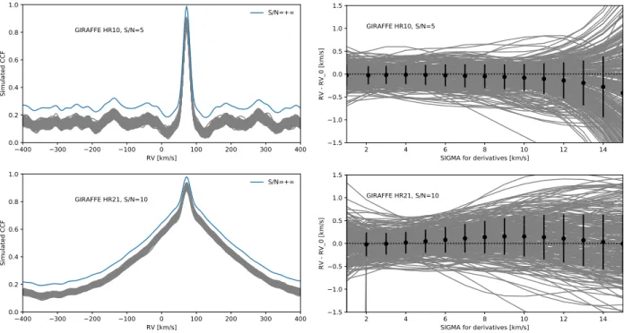
We performed Monte Carlo simulations to compute single-peak CCFs from spectra of different S/N but using the same at-mospheric parameters defined in Sect.3.2. We sliced this syn-thetic spectrum and degraded its resolution in order to match the following settings: GIRAFFE HR10 and HR21, UVES U520 and U580 (up and low). For each S/N level, we computed 251 re-alizations of our simulated GIRAFFE and UVES spectra by adding Gaussian noise and computed the corresponding CCFs using a mask made of a noise-free spectrum with a null radial ve-locity. We finally ran
doe
with different values of SIGMA (from 1 to 15 by step of 1 km s−1). Figures11and12show the dif-ference∆vrad = vrad,doe−vrad,0, wherevrad,0 = 72.0 km s−1, as a function of thedoe
parameter SIGMA (right panel) and the 251 CCFs (left panel) along with the noise-free CCF (labelled “+∞”). We show the results for the lowest S/N (i.e. the most un-favourable cases) for the setups GIRAFFE HR10 and HR21 and UVES U580 (low and up). The mean and standard deviation of∆vrad are also superimposed with dark dots and error bars in the right panels.
300 200 100 0 100 200 300 0.18
0.27 0.36
0.45 v1 = -16.36v2 = 19.3
v3 = 56.7
original
selection
300 200 100 0 100 200 300
0.5 0.0
0.51e 2
1st derivative
300 200 100 0 100 200 300
2 0 2
1e 4 w1 = 100.23 w2 = 100.23
w3 = 100.23
2nd derivative
300 200 100 0 100 200 300
v [km/s]
2 0 2
1e 5
3rd derivative
300 200 100 0 100 200 300
0.18 0.27 0.36
0.45 v1 = 18.31
original
selection
300 200 100 0 100 200 300
2 0 2
41e 3
1st derivative
300 200 100 0 100 200 300
1 0 1
21e 4w1 = 94.91
2nd derivative
300 200 100 0 100 200 300
v [km/s]
1.0 0.5 0.0 0.5 1.0 1e 5
3rd derivative
Fig. 10.Special procedure for fast rotators.Left panel: after few iterations three velocity components and one valley are detected.Right panel: after 11 iterations, one velocity component associated to one valley is identified. The associated spectrum hasS/N=65.
400 300 200 100 0 100 200 300 400
RV [km/s] 0.0
0.2 0.4 0.6 0.8 1.0
Simulated CCF
GIRAFFE HR10, S/N=5
S/N=+
2 4 6 8 10 12 14
SIGMA for derivatives [km/s] 1.5
1.0 0.5 0.0 0.5 1.0 1.5
RV - RV_0 [km/s]
GIRAFFE HR10, S/N=5
400 300 200 100 0 100 200 300 400
RV [km/s] 0.0
0.2 0.4 0.6 0.8 1.0
Simulated CCF
GIRAFFE HR21, S/N=10
S/N=+
2 4 6 8 10 12 14
SIGMA for derivatives [km/s] 1.5
1.0 0.5 0.0 0.5 1.0 1.5
RV - RV_0 [km/s]
GIRAFFE HR21, S/N=10
Fig. 11.Estimation of the accuracy of the radial velocities determined by the
doe
code on GIRAFFE setups HR10 and HR21 (Caii
triplet region). In each case, 251 simulated CCFs with a S/N as labelled and the blue line representing a noise-free CCF (left panels) were analysed withdoe
varying the value of SIGMA for the calculation of the smoothed successive derivatives and of the radial velocity (right panels).are less similar to the mask than the noise-free ones. In U580 (Fig.12), we see that the distance between the noisy CCFs and the reference value is not similar in the upper and lower left pan-els, despite the same S/N. A greater distance is seen in U580 low than in U580 up because there are more weak lines in the low setup for our simulated star, and therefore they quickly vanish in the noise when the S/N drops.
The right panels of Figs.11and12show the effect of SIGMA on the derived radial velocity (uncertainty and/or bias). Our simulations clearly demonstrate that SIGMA has to be chosen in a specific range to ensure reliable results. While our simulated
400 300 200 100 0 100 200 300 400 RV [km/s]
0.0 0.2 0.4 0.6 0.8 1.0
Simulated CCF
UVES U580l, S/N=5
S/N=+
2 4 6 8 10 12 14
SIGMA for derivatives [km/s] 1.5
1.0 0.5 0.0 0.5 1.0 1.5
RV - RV_0 [km/s]
UVES U580l, S/N=5
400 300 200 100 0 100 200 300 400
RV [km/s] 0.0
0.2 0.4 0.6 0.8 1.0
Simulated CCF
UVES U580u, S/N=5
S/N=+
2 4 6 8 10 12 14
SIGMA for derivatives [km/s] 1.5
1.0 0.5 0.0 0.5 1.0 1.5
RV - RV_0 [km/s]
UVES U580u, S/N=5
Fig. 12.Same as Fig.11for the UVES setups U580 low (Hβ+Mg I b triplet region) and U580 up (Hα+Na I D doublet region).
CCFs. Indeed, in Sect.2.1, we recall that the sampling frequency of the CCF is lower for GIRAFFE CCFs than for UVES CCFs: as SIGMA increases, a pronounced asymmetry on the second derivative appears for GIRAFFE CCFs, resulting in the high scatter displayed by Fig.11.
Our simulations allow us to quantify the effect of the S/N of the spectra on the method. For U520 and U580, the standard de-viation on the radial velocity at the recommended SIGMA goes from 0.05 km s−1 atS/N = 5 to lower than 0.01 km s−1 at S/N = 50. For GIRAFFE HR10, it goes from 0.20 km s−1 at S/N = 5 to 0.02 km s−1 atS/N = 50. For GIRAFFE HR21, the situation is the worst of all the setups with a standard de-viation going from 0.25 km s−1 atS/N = 10 to 0.06 km s−1 atS/N = 50. The obvious conclusion is that the UVES setups tend to give more precise results for a given S/N compared to the GIRAFFE setups. This is understandable since a single UVES spectrum has a higher resolution and a larger wavelength cov-erage than any GIRAFFE spectrum. For our simulated star, the precision on the radial velocity derived by
doe
is up to five times higher for UVES setups than for GIRAFFE HR10 (this is even worse when compared with HR21).This first approach of simulated CCFs shows that the method is quite robust with respect to the noise level in the GES spec-tra. Obviously, the presence of multiple components in the CCF may shift the detected radial velocities especially when the peaks blend with one another. In this case, the inaccuracy on the radial velocity can reach several km s−1 (increasing as the blending degree increases). No quantitative calculations have been per-formed so far, but the middle panel of Fig.7shows a good ex-ample: the main peak is detected at 0.95 km s−1of its expected position and the second peak at 2.3 km s−1, with a simulated distance of 24 km s−1 between the two peaks. We conclude that the (conservative) random uncertainty on the radial veloc-ity derived by
doe
is of the order of±0.25 km s−1, while the systematic uncertainty is lower than 0.05 km s−1for single-peak CCFs and may reach a few km s−1 for multi-peak CCFs. Other effects, like template mismatch or imperfect normalization, may have an effect on the uncertainty on the derived radial velocity.We also refer the reader to Jackson et al. (2015) where a dis-cussion on the radial velocity uncertainties can be found, along with their empirical calibrations as a function of S/N, vsini, and the effective temperature of the source for GIRAFFE HR10, HR15N, and HR21 setups. As shown bySacco et al.(2014) and Jackson et al.(2015), the errors on the GES radial velocities for most of the stars are dominated by the zero-point systematic er-rors of the wavelength calibration, which are not discussed here.
3.5. Detection efficiency as a function of S/N
Using Monte Carlo simulations, we assessed the impact of the S/N of GIRAFFE HR10 and HR21 spectra on the detection ef-ficiency of the double-peaked CCF of an SB2. For that purpose we simulated synthetic SB2 spectra (a pair of twin stars) varying the S/N (from 1 to 100) and varying the difference in radial ve-locity of the two components∆vrad (from 5 to 100 km s−1). For each pair (∆vrad, S/N), we computed as above 251 realizations of the spectra and their corresponding CCFs. We then applied
doe
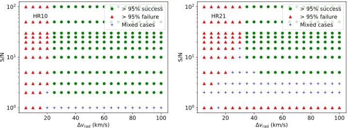
with the parameters adapted to each setup (see Table1).The maps in Fig.13show the detection efficiency in HR10 and HR21. The green dots (respectively, the red triangles) indi-cate (∆vrad, S/N) conditions when
doe
is able to detect the two expected peaks in more than 95% of cases (respectively, condi-tions whendoe
failed to detect the two expected peaks in more than 95% of cases). Blue plusses represent intermediate cases making detection efficiency dependent on the noise: due to the noise, spurious peaks may appear (i.e. detection failed) or the two peaks may have different heights (despite being twin stars) and become discernible todoe
for small∆vrad(i.e. detection suc-ceeded; e.g. for HR21, atS/N=10 and∆vrad=25 km s−1).These simulations demonstrate that even spectra with very low S/N carry sufficient information to reveal the binary na-ture of the targets. Specifically, in the HR10 setup, double peaks are detected in 95% of the cases when S/N ≥ 2 and
20
40
60
80
100
v
rad(km/s)
10
010
110
2S/N
HR10
> 95% success
> 95% failure
Mixed cases
20
40
60
80
100
v
rad(km/s)
10
010
110
2S/N
HR21
> 95% success
> 95% failure
Mixed cases
Fig. 13.Assessement of the
doe
detection efficiency of the two radial velocity components of simulated SB2 CCFs as a function of the S/N and the radial velocity differences for GIRAFFE HR10 (left panel) and HR21 (right panel) setups.the S/N threshold that we adopted (i.e. analysis of CCFs for all spectra withS/N ≥ 5) protect us from mixed cases, which tend to happen for the lowest levels of S/N. This also shows that the HR10 setup is more able to detect SB2 than HR21 because HR21 is located around the IR Ca
ii
triplet whose lines have strong wings that decrease the detection efficiency. In Sect.4.2, the histogram of the radial velocity separation of the effectively detected SB2 candidates is presented (Fig.18). Observationally, HR10 spectra (respectively, HR21) allow us to detect SB2 with∆vradas low as∼25 km s−1(respectively,∼60 km s−1): for both setups we are dealing with cases falling in the green dotted area of the maps. Thus, we expect in all cases an SB2 detection effi -ciency better than 95%.
4. iDR4 results and discussion
The
doe
code is included in a specifically designed workflow to handle all the GES single-exposure spectra for all setups. The automated workflow includes three steps: first, the CCFs are se-lected using the set of criteria described in Sect.2.2; second, thedoe
code is applied to the CCFs to identify the number of peaks and a confidence flag is assigned; third, the CCFs in a given setup are combined per star and a last criterion is applied: for a given star, if more than 75% of the CCFs in at least one setup show two peaks (respectively, three and four), then the star is classified as SB2 candidate (respectively, SB3 and SB4). This rather restric-tive criterion (see Sect.4.7) is adopted to prevent false positive SB detections (due to spectra normalization, cosmics, nebular lines, etc.).After this automatic procedure, a visual inspection is per-formed to ensure that no false positive detection remains and that the confidence flag is relevant. We investigate the CCFs and the spectra of all the SBn candidates one by one. When a clear false detection is encountered, the SB candidate is removed from the list. When an SB is flagged by the automatic process as probable (A) or possible (B), but the visual inspection of the CCF series (all setups considered) casts doubts on this classifi-cation, the corresponding spectra for that object are inspected. The choice of the final flag for an object can be downgraded if other CCFs provide discrepant results. This procedure en-sures that processes other than binarity moderately contaminate SB candidates flagged C, marginally contaminate SB candidates
Fig. 14.Magnitude distributions of SB2 systems from theNinth Cat-alogue of Spectroscopic Binary Orbits(dashed line), downloaded in September 20165, and in the GES (solid line). GES SB3 systems are shown as the dotted-line.
flagged B, and exceptionally contaminate those flagged A. De-spite these difficulties, adopting clear classification criteria en-sures the best possible consistency throughout the survey.
20 10 0 10 20 30 40 50
ccf_3p_10_15_20.dat (5000) [THRES0 = 30 %, THRES2 = 10 %, SIGMA = 3.00] original
ccf_3p_10_14_20.dat (5000) [THRES0 = 30 %, THRES2 = 10 %, SIGMA = 3.00] original
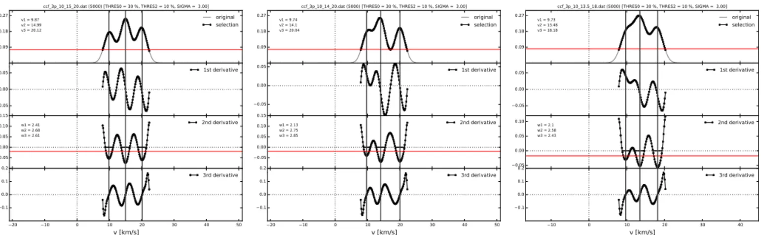
ccf_3p_10_13.5_18.dat (5000) [THRES0 = 30 %, THRES2 = 10 %, SIGMA = 3.00] original
Fig. 15.Triple-peak simulated CCFs with a main peak fixed at 10 km s−1detected with confidence flags A (left; second and third peaks at 15 and 20 km s−1), B (middle; second and third peaks at 14 and 20 km s−1), and C (right; second and third peaks at 13.5 and 18 km s−1).
open clusters, and toPancino et al.(2017) for the criteria in glob-ular clusters and calibration open clusters. We note that the tar-gets observed in regions like the bulge, Cha I (Sacco et al. 2017), andγ2Vel (Prisinzano et al. 2016) associations, as well as theρ Oph (Rigliaco et al. 2016) molecular cloud, are selected on the basis of coordinates and photometry (VISTA and 2MASS), thus providing a rough membership criterion.
The list of the SB2 and SB3 candidates in the Milky Way field is given in TablesA.1andA.2. The list of SB2 in the bulge, the Cha I,γ2 Vel, andρOph associations and the CoRoT field is given in TableB.1. Finally, the list of SBn in stellar clusters is given in TableC.1. The results (classifications and confidence flags) are included in the GES public releases (see footnote 3) using the nomenclature given in the GES outlier dictionary de-veloped by the GES Working Group 14 (WG 14)6.
4.1. Binary classification
The binary classification7 was developed for the GES within WG 14. The following scheme is adopted: the peculiarity flag is built from the juxtaposition of a peculiarity index and a confi-dence flag letter. The peculiarity index is defined as 20n0, with n ≥ 2, wherenis the number of distinct velocity components in the CCF. With this peculiarity index, an SB2 is classified as 2020, an SB3 2030, etc. Even though a star is flagged 2020 (i.e. SB2), a third component may be present but not visible during the observation or may be undetectable at the resolution and S/N of the considered exposure.
Moreover, the WG14 dictionary recommends the use of con-fidence flags (A: probable, B: possible, and C: tentative). Clearly, the closer the CCF peaks are, the less certain the detection is. The criteria to allocate these flags were defined as follows:
– A: the local minimum between peaks is deeper than 50% of the full amplitude of the highest peak;
– B: the local minimum between peaks is higher than 50% of the full amplitude of the highest peak;
– C: no local minimum is detected between peaks, but the CCF slope changes.
6 The aim of WG 14 is to identify non-standard objects which, if not properly recognized, could lead to erroneous stellar parameters and/or abundances. A dictionary of encountered peculiarities has been created, allowing each node to flag peculiarities in a homogeneous way. 7 See footnote3.
Table 2.Number of SB2, SB3 and SB4 candidates per confidence flag.
Confidence flag
Peculiarity index A B C Total SB2 (2020) 127 107 108 342
SB3 (2030) 7 1 3 11
SB4 (2040) 1 0 0 1
Notes.A: probable, B: possible, C: tentative.
With these definitions, the SB2 whose CCF is plotted in the left, middle, and right panels of Figs.8and9would be flagged as A, B, and C, respectively.
For triple-peak CCFs, the same type of criteria are applied to the second local minimum. If this second local minimum is lower than 70% of the full amplitude of the highest peak, then the confidence flag is set to A, else B. Examples of these two cases are shown on simulated CCFs in Fig.15. The CCF in the middle panel is classified as 2030B because the leftmost local minimum is higher than 0.5 times the largest amplitude, but also as 2020A because the middle and leftmost peaks, taken as a whole, are well separated from the rightmost peak.
4.2. iDR4 SB2 candidates
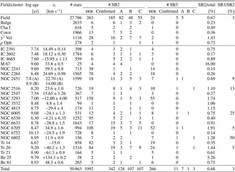
Table 3.Distribution of SB2 and SB3 candidates among the different observed fields.
Field/cluster log age vr # stars # SB2 # SB3 SB2/total SB3/SB2
[yr] [km s−1]
doe
Confirmed A B Cdoe
Confirmed A B C [%] [%]Field 27 786 263 185 82 48 55 24 5 5 0.67 3
Bulge 2633 6 6 1 3 2 0 0 0.23
Cha I 616 5 2 2 1 0 0.49
Corot 1966 13 7 5 2 0 0 0.36
γ2Vel 1116 28 16 2 7 7 2 0 1.43
ρOph 278 2 1 1 1 0 0.72
IC 2391 7.74 14.49±0.14 398 4 3 2 1 4 0 0.75
IC 2602 7.48 18.12±0.30 1784 6 3 1 1 1 3 0 0.17
IC 4665 7.60 −15.95±1.13 559 6 5 2 2 1 1 0 0.89
M 67 9.60 33.8±0.5 25 4 4 4 0 0 16.00
NGC 2243 9.60 59.5±0.8 715 38 1 1 14 0 0.14
NGC 2264 6.48 24.69±0.98 1565 78 4 2 2 18 0 0.26
NGC 2451 7.8 (A) 22.70 (A) 1599 18 11 3 5 3 7 1 1 0.69 9
8.9 (B) 14.00 (B)
NGC 2516 8.20 23.6±1.0 726 19 8 1 4 3 10 1 1 1.10 13
NGC 2547 7.54 15.65±1.26 367 7 1 1 3 0 0.27
NGC 3293 7.00 −12.00±4.00 517 158 9 1 5 3 55 0 1.74
NGC 3532 8.48 4.8±1.4 94 1 1 1 0 0 1.06
NGC 4815 8.75 −29.4±4 174 11 2 1 1 0 0 1.15
NGC 6005 9.08 −24.1±1.3 531 12 4 2 1 1 8 1 1 0.75 25
NGC 6530 6.30 −4.21±6.35 1252 95 5 2 3 1 0 0.40
NGC 6633 8.78 −28.8±1.5 1643 17 15 3 7 5 0 0 0.91
NGC 6705 8.47 34.9±1.6 994 108 19 5 3 11 52 1 1 1.91 5
NGC 6752 10.13 −24.5±1.9 728 8 1 1 0 0 0.14
NGC 6802 8.95 11.9±0.9 156 7 2 2 7 1 1 1.28 50
Tr 14 6.67 −15.0 858 82 3 2 1 19 0 0.35
Tr 20 9.20 −40.2±1.3 1316 84 19 3 7 9 24 1 1 1.44 5
Tr 23 8.90 −61.3±0.9 164 5 1 1 5 0 0.61
Be 25 9.70 +134.3±0.2 38 2 2 2 1 0 5.26
Be 81 8.93 48.3±0.6 265 5 2 1 1 6 0 0.75
Total 50 863 1092 342 128 107 107 266 11 7 1 3 0.68 3
Notes. The column “log age” lists the logarithm of the cluster age (in years) fromCantat-Gaudin et al.(2014; NGC 6705), Spina et al. (in prep.; IC 2391, IC 2602, IC4665, NGC 2243, NGC 2264, NGC 2541, NGC 2547, NGC 3293, NGC 3532, NGC 6530),Bellini et al. (2010; M 67),Bragaglia & Tosi(2006; NGC 2243),Sung et al.(2002; NGC 2516),Friel et al.(2014; NGC 4815),Jacobson et al.(2016; NGC 6005, NGC 6633),VandenBerg et al.(2013; NGC 6705),Tang et al.(2017; NGC 6802),Donati et al.(2014; Tr 20 and Berkeley 81, written Be 81),
Overbeek et al.(2017; Tr 23), and Carraro et al.(2007; Be 25). The columnvr lists the radial velocity; for the clusters with ages older than 100 Myr seeJacobson et al.(2016, only UVES targets) excepted for M 67 (Casamiquela et al. 2016), NGC 2243 (Smiljanic et al. 2016);Friel et al.
(2014; NGC 4815),Harris(1996; NGC 6752). For the young clusters, seeDias et al.(2002; IC 2391, IC 2602, IC 4665, NGC 2264, NGC2451, NGC 2547, NGC 3293, NGC 6530), andCarraro et al.(2007; Be 25). The column “# stars” lists the number of stars in that particular field/cluster observed by the GES. The column “
doe
” gives the number of SBs detected automatically, whereas the column “confirmed” represents the number of SBs kept after visual inspection of CCFs and associated spectra. The columns labelled “A”, “B”, and “C” list the number of confirmed systems by confidence flag (probable, possible, and tentative, respectively). No SB2 or SB3 candidates have been found yet with thedoe
code for the following clusters within the GES: Be 44 (93), M 15 (109), M 2 (110), NGC 104 (1138), NGC 1851 (127), NGC 1904 (113), NGC 2808 (112), NGC 362 (304), NGC 4372 (120), NGC 4833 (102), and NGC 5927 (124), where the numbers in parentheses give the number of stars observed in each cluster.Moreover, emission in the line cores of this triplet induces fake double-peak CCFs because in the templates the lines are always in absorption. Consequently, it is very difficult to identify double peaks due to binarity based on HR21 CCFs (see Sect.4.7 for more details). This explains why we only have two firm de-tections among the 31 970 stars observed with this setup alone. Hence, this setup is not well-suited to detecting stellar multiplic-ity at least in our situation (see Matijeviˇc et al. 2010: although they were able to discover 123 SB2 out of 26 000 RAVE targets, they also had to deal with very broadened CCFs and could not detect binaries with∆vrad≤50 km s−1).
The setup with the second largest number of observed ob-jects is HR10. This setup covers the range [535−560] nm with many small absorption lines that result in a narrow CCF, suitable for the detection of stellar multiplicity (see Fig.8). The largest number of probable SB2 candidates is indeed detected with this setup.
setups where the composite nature of the spectrum is clearly vis-ible in Fig.16).
Contrary to field stars, which are observed in HR10 and HR21 only, cluster stars were observed with many different setups. The number of SB2 candidates in the field is 185 out of 27786 stars (0.67%) whereas in the clusters it amounts to 127 out of 16468 (0.77%, see Table3).
There are about 30 SB2 candidates detected with a double-peaked CCF in both GIRAFFE HR10 and HR21. For instance, the field star 02394731-0057248 (magnitudeV =13.8) is iden-tified as an SB2 candidate with HR10 and HR21 (see Fig.17). This new candidate has no entry in the Simbad database.
The histograms of the radial velocity separation of SB2 can-didates for GIRAFFE HR10 and HR21 and for UVES U580 are shown in Fig. 18(U520 is not represented, due to insufficient statistics). The smallest measured radial velocity separations are 23.3, 60.9, and 15.2 km s−1for HR10, HR21, and U580, respec-tively. This is well in line with the detection capabilities of the
doe
code as mentioned in Sect.3.3(∼30 km s−1for GIRAFFE and∼15 km s−1for UVES setups). In U580, the high bin value around 72 km s−1 is mainly due to the repeated observations of a specific object, the SB4 candidate 08414659-5303449 in IC 2391 (see Sect.4.5).Concerning the SB2 candidates in open clusters, not only did we check the cleanliness of the SB2 CCF profile, but we also compared the velocities of the two peaks with the cluster veloc-ity. Assuming that most of the SB2 systems discovered by GES generally have components of about equal masses, then an SB2 that is member of the cluster should have a cluster velocity about midway between the two component velocities. This simple test allows us to assess the likelihood that the SB2 system is a cluster member. This method is applied for the SB2, SB3, and SB4 can-didates analysed and full details are given in the present section and in Sects.4.4and4.5. The results are shown in TableC.1. The column labelled “Member” in TableC.1evaluates the likelihood of cluster membership based on the component velocities: if the cluster velocity falls in the range encompassed by the compo-nent velocities, we assume that the centre of mass of the system moves at the cluster velocity, which means that membership is likely. In that case, we put “y” in the column. On the contrary, if the CCF exhibits two well-defined peaks not encompassing the cluster velocity, the star is labelled as an SB2 non-member of the cluster (“n” in the column). Another possibility is that one com-ponent has a velocity close to that of the cluster and the second velocity is offset. In that case, the SB2 nature is questionable and the star is more probably a pulsating star (responsible for the secondary peak or bump) belonging to the cluster (“y” in col-umn “Member”). The list of individual radial velocities based on iDR5 data will be given in a forthcoming paper. More extended remarks for each cluster are provided in AppendixC.
4.3. Orbital elements of two confirmed SB2 in clusters
With the data collected so far, we were able to confirm the binary nature of two SB2 candidates in clusters by deriving reliable or-bital solutions for the systems 06404608+0949173 (NGC 2264 92) and 19013257-0027338 (Berkeley 81, hereafter Be 81).
The first system 06404608+0949173 (magnitudeV∼ 12) is a bona fide SB2 for which 24 spectra are available (20 GIRAFFE HR15N and 4 UVES U580) and an orbit can be computed, as shown in Fig.19. Observations where only one velocity com-ponent is detected are not used to calculate the orbital solution because these velocities are not accurate (Fig.19) since the two velocity components are blended. The orbital elements are listed
in Table4. The short period of 2.9637±0.0002 d implies that nei-ther of the components can be a giant, which is consistent with the classification of the system as K0 IV (Walker 1956). The centre-of-mass velocity of the system (14.6 km s−1) is close to the cluster velocity (17.7 km s−1), as it should be. The mass ratio isMB/MA=1.10. Classified as FK Com in the GCVS (=V642 Mon), this source is chromospherically active with X-ray emis-sion (ROSAT and XMM). This system thus adds to the two SB2 systems with available orbits (VSB 111 and VSB 126) already known in NGC 2264 (Karnath et al. 2013).
The second system 19013257-0027338 (magnitudeV ∼17) is a confirmed SB2 (2020 A) for which 18 spectra are available (8 GIRAFFE HR15N and 10 GIRAFFE HR9B). This source is not listed in the Simbad database. The orbital elements are given in Table4and the orbit is displayed in Fig.20. Strangely enough, a good SB2 solution for this system could only be obtained by adding an extra parameter to the orbital elements, namely an offset between the systemic velocities derived from compo-nent A and from compocompo-nent B (see the∆VB term in Eq. (2) of Pourbaix & Boffin 2016). In most cases this offset is null, but there could be situations where it is not, like in the presence of gravitational redshifts or convective blueshifts that are dif-ferent for components A and B (Pourbaix & Boffin 2016). Al-ternatively, if the spectrum of one of the components forms in an expanding wind (as in a Wolf-Rayet star), it would also lead to such an offset. However, what is puzzling in the considered case is the large value of the offset (24.8±1.2 km s−1) for which we could not find any convincing explanation. Indeed, no Wolf-Rayet stars are known in the Be 81 cluster according to the Sim-bad database. This very diffuse cluster of intermediate age lies towards the Galactic centre (Hayes & Friel 2014; Donati et al. 2014).
4.4. SB3 candidates
Tables2and3show that, in total, 11 SB3 candidates (7 probable: flag A, 1 possible: flag B, and 3 tentative: flag C) were detected. Five of these SB3 are found in the field (Fig.21and TableA.2) and six in clusters (Fig. 22 and within Table C.1). A total of 266 targets were initially labelled as SB3 candidates by the
doe
code, while only 11 were kept after visual inspection, giving a success rate of about 4% (compared to 30% for SB2 detection). The SB3 candidates are essentially detected in UVES setups and in GIRAFFE setups HR9B and HR10. The SB3 candidates in the stellar clusters were examined on a case-by-case basis, and the results are reported below.NGC 2451. The CCF of 07470917-3859003 exhibits three clear peaks (the CCF is classified as 2030A), at 25.0, 96.1, and 136.6 km s−1. The first velocity is compatible with member-ship in NGC 2451A. The DSS8 image reveals the presence of a slightly fainter star about 1200south (a greater distance than the 1.200 size of the fibre, so no contamination is possible). Given the fact that the two fainter peaks are not located symmetrically with respect to the cluster velocity, it is doubtful that the system could be a physical triple system in the case of membership to NGC 2451.
NGC 2516. NGC 2516 45 (system 07575737-6044162) is a star classified as A2 V (Hartoog 1976) withV =9.9. The iDR4 8 Digitized Sky Survey:https://archive.stsci.edu/cgi-bin/
4040 4060 4080 4100 4120 4140 4160 4180
4550 4600 4650 4700 4750
[Å]
5150 5200 5250 5300 5350
[Å]
5350 5400 5450 5500 5550 5600
[Å]
6350 6400 6450 6500 6550 6600 6650
[Å]
6450 6500 6550 6600 6650 6700 6750 6800
[Å]
8500 8600 8700 8800 8900
[Å]
300 200 100 0 100 200 0.0
0.1 0.2
0.3 v1 = -58.7
v2 = 21.36
original
selection
300 200 100 0 100 200
0.5 0.0 0.5 1.01e 2
1st derivative
300 200 100 0 100 200
0.9 0.0 0.9
1e 3 w1 = 24.84
w2 = 29.78
2nd derivative
300 200 100 0 100 200
v [km/s]
0.9 0.0 0.9
1.81e 4
3rd derivative
400 200 0 200 400
0.0 0.2 0.4 0.6
v1 = -62.93
v2 = 22.14
original
selection
400 200 0 200 400
0.5 0.0
0.51e 2
1st derivative
400 200 0 200 400
2 0 2
41e 4w1 = 46.23
w2 = 55.93
2nd derivative
400 200 0 200 400
v [km/s]
2 0 2 4 1e 5
3rd derivative
Fig. 17.Example of identification of a new SB2 candidate 02394731-0057248 not reported in Simbad.Left panel: GIRAFFE HR10 setup (S/N∼
10).Right panel: GIRAFFE HR21 setup (S/N∼140).
0 50 100 150 200 250 300
RV [km/s]
020 40 60 80 100 120
N
U580 (411)
HR10 (225)
HR21 (177)
Fig. 18. Radial velocity separation of SB2 candidates for GIRAFFE HR10, HR21, and for UVES U580 single exposures. The numbers in parentheses are the numbers of single exposures where two peaks were identified.
recommended parameters (Teff =8500 K, logg =4.1, and so-lar metallicity) suggest that it could be aδScu star. Its CCF is most likely associated with a fast rotator with a superimposed sharper central peak. The SB3 nature of this candidate is there-fore doubtful and a follow-up of this source should be performed before drawing any firm conclusion.
NGC 6705. In total, the
doe
routine finds 52 SB3 candi-dates in NGC 6705, one of the largest number of SB3 among all the targeted clusters (Table 3). After a first-pass analysis we discarded all of them but one, NGC 6705 1147 (system 18510286-0615250). The velocities corresponding to the three peaks observed in the CCF are listed in Table5. They exhibit clear temporal variations. The cluster velocity is 29.5 km s−1 (Cantat-Gaudin et al. 2014). This velocity is close to that of the middle peak in the CCF (C, i.e. the faintest). That central peak0.0 0.2 0.4 0.6 0.8 1.0
Phase 100
50 0 50 100
Radial velocity [km/s]
CNAME 06404608+0949173 Component A Component B Unidentified
Fig. 19. SB2 orbit of 06404608+0949173 in NGC 2264. Compo-nent A is represented by large circles and compoCompo-nent B by small cir-cles. Squares represent the single radial velocity obtained when only one peak is visible in the CCF; these are not used to calculate the orbital solution, due to their larger uncertainties. The error on radial velocities amounts to±0.25 km s−1. The horizontal dotted line isV
0.
does not vary as much as the most extreme peaks, and moreover, the shape of peak C is not as sharp as are peaks A and B. Consid-ering that the cluster NGC 6705 is a dense one, we believe that this third peak is from background contamination. We therefore conclude that the detection of NGC 6705 1147 as SB3 is spu-rious and should be downgraded to SB2. The SB2 analysis is presented in Table5where we computed the mass ratio, adopt-ing 34 km s−1(Table3) as the centre-of-mass (cluster) velocity. The observed velocity variations are consistent at all times with a mass ratio of the order of 1.32.
Table 4.Orbital elements for 06404608+0949173 in NGC 2264, and 19013257-0027338 in Be 81.
CNAME 06404608+0949173 19013257-0027338 P(d) 2.9637±0.0002 15.528±0.002 e 0.092±0.006 0.170±0.006
ω(◦) 56.8±3.9 265.7±3.9
T0– 2 400 000 (d) 56072.4085±0.0351 56470.531±0.140 V0(km s−1) 14.32±0.55 34.51±0.66
∆VB 0.00 (adopted) 24.8±1.2 KA(km s−1) 106.3±0.7 86.0±0.9 KB(km s−1) 117.0±0.6 97.0±0.9
σA(O−C) (km s−1) 20.2 6.1
σB(O−C) (km s−1) 9.3 6.8
aAsini(Gm) 4.315±0.030 18.1±0.2 MA/MB 1.10 1.13
N 16 18
Notes. The orbital elements are the orbital periodP, the eccentricitye, the argument of the periastronωfrom the ascending node, the time of passage at periastronT0, the velocity of the centre-of-massV0, the primary and secondary velocity amplitudesKAandKB, the projected primary semi-major axis on the plane of the skyaAsiniand the primary to the secondary mass ratioMA/MB.σA(O−C) andσB(O−C) are the standard deviation of the residuals (observed−calculated) of components A and B.Nis the number of avalaible CCFs on which two velocity components are identified. For the meaning of∆VBsee Eq. (2) ofPourbaix & Boffin(2016).
Table 5.Velocities of the three peaks (A, B, C) in the CCF of NGC 6705 1147.
JD – 2 456 000 Setup vr(A) vr(B) vr(C) ∆vr(A) ∆vr(B) MA/MB 77.409 HR3 79.62 −24.70 33.83 45.62 58.70 1.29 99.268 HR3 95.35 −47.33 29.87 61.35 81.33 1.33 99.280 HR5A 95.38 −45.73 23.68 61.38 79.73 1.30 99.295 HR6 93.65 −44.84 35.92 59.65 78.84 1.32 99.298 HR9B 94.83 −46.62 40.28 60.84 80.62 1.33 103.110 HR10 −26.78 106.91 39.14 60.78 72.91 1.20 442.394 HR10 75.38 −18.75 40.61 41.38 52.75 1.27 442.400 HR10 72.20 −20.23 26.72 38.20 54.23 1.42 442.406 HR10 75.41 −22.23 33.44 41.41 56.23 1.36
Notes.The columns labelled∆list the differential velocity with respect to the centre-of-mass (i.e. cluster) velocity, adopted as 34 km s−1.
0.0 0.2 0.4 0.6 0.8 1.0
Phase 50
0 50 100 150
Radial velocity [km/s]
CNAME 19013257-0027338 Component A Component B
Fig. 20.SB2 orbit of 19013257-0027338 in Berkeley 81. Component A is represented by large circles and component B by small circles. The error on radial velocities amounts to±0.25 km s−1. The horizontal dot-ted line isV0.
(Carlberg 2014). The spectra are at the minimum required S/N. These data are compatible with 15553867-5724434 being an SB3 member of NGC 6005.
NGC 6802. The CCF of 19302315+2013406 (classified as 2030C) shows three distinct peaks, at −22.4, 22.0, and 65.5 km s−1, compared with 12.4 km s−1 for the cluster ve-locity (Hayes & Friel 2014). These data are compatible with 19302315+2013406 being an SB3 member of NGC 6802.
Trumpler 20. The CCF of 12391904-6035311 (classified as 2030C) shows three distinct peaks, at −85.78, −44.4, and 14.8 km s−1, compared with−40.8 km s−1 for the cluster ve-locity (Kharchenko et al. 2005). These data are compatible with 12391904-6035311 being an SB3 member of Trumpler 20. An extended analysis of the GES data for this cluster may be found inDonati et al.(2014).
4.5. The unique SB4 candidate HD 74438
We detected one SB4 candidate: the A2V star HD 74438 (CNAME 08414659-5303449, withV =7.58) belonging to the open cluster IC 2391 (Platais et al. 2007).
Table 6.Velocities of the four peaks (A, B, C, D) in the CCF of HD 74438 over the night of February 18, 2014, obtained with the U580 setup. Notes.The columns labelled∆list the differential velocity with respect to the centre-of-mass (i.e. cluster) velocity.
400 300 200 100 0
100 200 300 400
Fig. 21.CCFs of the five SB3 candidates (flagged 2030 A) in the field. Velocities of the components are given in km s−1.
deviation for a binary system with two components of equal brightness would amount to 2.5 ×log 2 = 0.75 mag). It is nevertheless considered a bona fide member of the cluster by Platais et al.(2007). Therefore, the centre-of-mass velocity for the system can be considered identical to the cluster velocity, namely 14.8 ±1 km s−1 (Platais et al. 2007). A typical exam-ple of the CCF of HD 74438 is presented in Fig.23where its four distinct CCF peaks are clearly apparent. The velocities of the peaks at different times over the night of February 18, 2014, are collected in Table6. In this table, we first notice that the ve-locities of components A and B (which correspond to the highest peaks) vary slowly and oppositely to each other. Their amplitude of variations is similar. If we compute the velocity variations with respect to the cluster velocity (which should correspond to the centre-of-mass velocity of the AB pair, neglecting the gravi-tational influence of components C and D – columns∆vr(A) and
400 300 200 100 0
100 200 300 400
6
07470917-3859003 (NGC 2451)
U580
S/N = 84
Fig. 22.CCFs of the six SB3 candidates in the stellar clusters. Velocities of the components are given in km s−1. The vertical scale of the CCFs has been magnified for clarity.