Dynamic model of the value stream in a power

Texto completo

(1)Heurística 16, Noviembre 2009, p.91-104. DYNAMIC MODEL OF THE VALUE STREAM IN A POWER GENERATION SYSTEM THAT RUNS ON A FOSSIL FUEL. Oscar Rubiano Ovalle Universidad del Valle, Escuela de Ingeniería Industrial y Estadística, Cali oscaruba@pino.univalle.edu.co. Alejandro Peláez De Lee Ingeniero Químico, Colombia apelaez_de_lee@hotmail.com. Abstract Power generation systems are usually employed in the chemical process industry and in mechanical and electrical processes as well. The value stream that makes up these processes is based upon energy generation with turbo machinery that is powered by steam. Coal is the fuel used to furnish the steam in the power plant pilot of this research. This research allowed the construction of a dynamic model that works as an analytical tool both for the constituents of a power generation system, and for the power generation system as a whole. The objective was to study the performance of a power system that provides thermodynamic work. Results show that simulation using system dynamics is a powerful tool that can assist power generation system studies. The investigation reveals the important effect of coal’s oxidation on the value stream of power generation systems. The fuel’s calorific value depends on the coal inventory, i.e. on the amount of time it is stored. Keywords: Value Stream, Combustion, Simulation, System Dynamics.. Resumen Los sistemas generadores de energía térmica son comúnmente empleados en la industria de procesos químicos, mecánicos y eléctricos. La cadena de valor en la cual subyacen estos procesos térmicos, se fundamenta en la generación de la energía a partir de vapor. El vapor requerido en el caso objeto de estudio de esta investigación se obtiene usando carbón como insumo. Esta investigación permitió construir un modelo dinámico que sirva como instrumento de análisis del sistema de generación de energía como un todo, así como de sus elementos. El objetivo fue estudiar el desempeño del sistema de generación de energía que suministra trabajo termodinámico. Los resultados muestran que la simulación con Dinámica de Sistemas es una poderosa herramienta de estudio de los sistemas de generación de energía. La investigación muestra el alto impacto de la oxidación del carbón en la cadena de valor de los sistemas de generación de energía. El poder calorífico del carbón utilizado en la producción del vapor depende del inventario de carbón, es decir, de su tiempo de almacenamiento. Palabras Clave: Cadena de Valor, Combustión, Simulación, Dinámica de Sistemas.. 91.

(2) Rubiano, O., Peláez, A. – Dynamic model of the value stream in a power generation …. 1.. Introduction. The fuel load depends on the efficiency of the heat transfer process required in the boiler. Coal’s combustion reaction is commonly used to yield thermal energy. During the combustion of this fuel, Carbon (one of the elements that make up coal, and the one responsible for its power), turns into Carbon Dioxide (CO2) and Carbon Monoxide (CO). This reaction releases a considerable amount of energy that is supplied to the water inside the boiler. The water in liquid state then turns into steam during the heat transfer process. Unlike other fossil fuels, coal decays during the time it is stored. Coal reacts spontaneously with the surrounding air and oxidizes, a phenomenon known as spontaneous combustion. As a result coal loses its chemical properties and therefore, lowers its available BTUs. During this process Coal also loses its economic value because its cost relates directly to its calorific capacity. The longer the time this fuel is stored, the more the coal degrades, and thus more money will be spent by management, replacing the degraded coal with a better one. Longer storage periods entail a deterioration of the fuel’s quality and thus reduce the ratio of steam output per coal fed into the system. Even though coal is widely used as fuel in combustion processes, the economic effect of its spontaneous reaction with air hasn’t been studied thoroughly. Some well known supply chain academic authors like Sipper (1997) and Ballou (2004) don’t deal with this subject. The academic research usually concentrates on the reaction kinetic of the spontaneous combustion and its relationship to safety topics and not on its economic impact (Smith and Glasser, 2005, and Krishnaswamy et al., 1996). Some authors address their investigations on root cause analysis related to the physical and chemical characteristics that influence this reaction (Brooks y Glasser, 1986 and Pone et al., 2007). In the subject plant, coal is stacked in big piles and then it is fed to the boiler.. 92. 2.. Review of the Mass and Energy Balance and the Modeling of Physical and Chemical Processes with System Dynamics. Hougen et al. (1982) reviewed specifically the mass and energy balance associated to the combustion of this fuel. Other authors such as Himmelblau (1997) and Reklaitis (1989) apply numerical calculus to solve the equations that make up the mass and energy balance. Energy balances associated to the combustion reaction have been thoroughly revised by Bejan (1997) and Smith et al. (2007). Spontaneous combustion is a low temperature oxidation that has been studied primarily for its potential to turn stored coal into a fire. This phenomenon is a chain reaction where the magnitude of the fire depends on the amount of fuel stored. Smith and Glasser (2005) and Krishnaswamy et al. (1996) study the factors that have an effect on the kinetic of the chemical reaction. In these studies, Krishnaswamy et al. (1996) develop a mathematical bidimensional model to analyze several factors such as the porosity of the coal pile, the inclination angle of the pile, and the particle size of the coal. Brooks and Glasser (1986) formulate a mathematical model with three differential equations for the temperature, pressure gradient, and the oxygen concentration in the coal pile. In their investigation Brooks and Glasser also reviewed the effects of the particle size of the fuel, and the porosity of the coal pile. Beamish and Arisoy (2008) proposed a model for the kinetic of the reaction and its relationship with temperature; however this model is different from Svante Arrhenius’ (Chemistry Nobel prize winner, 1903) equation. Smith and Glasser (2005) analyze other factors that are important, like the fuel’s calorific capacity, the heat of reaction and the activation energy of the combustion reaction. According to their research, these properties don’t vary between coals of different rank (different calorific value). Additionally, their investigation.

(3) Heurística 16, Noviembre 2009, p.91-104. concluded that the reaction rate between the fuel and oxygen are correlated with the coal’s chemical composition. In another research Pone et al. (2007) examines the chemical composition of the combustion gases and ashes during the fuel’s low temperature oxidation. None of the research discussed before, associates spontaneous combustion to its economic consequences. Fierro et al. (1998) is one of the few researchers that conducted an investigation that linked this phenomenon and money. In this study the authors tested several experiments to minimize spontaneous combustion, such as shaping coal piles with low inclination angles, compressing the pile periodically, placing a physical barrier to the pile and adding ash slurry in order to lower the heat loss transferred to the surroundings. The best results where obtained when the slurry was added to the coal pile. None of the papers established a relationship between spontaneous combustion and a power a generation system, and none of the research discussed spontaneous combustion topics and System Dynamics. System Dynamics is a methodology that helps study complex systems that are time dependent. These systems can be expressed mathematically with differential equations and can be integrated with numerical calculus (Sterman, 2000). The mass and energy balances are physical processes that may be modeled by non linear ordinary differential equations. These reasons explain why System Dynamics is an appropriate methodology to study physical and chemical systems such as the power generation by the combustion of coal in a boiler. In the following section, System Dynamics is introduced as a tool for modeling physical and chemical processes, then in section 4 and in section 5 the power generation system is modeled. In section 5 the model is validated with process data. Section 6 presents the results, and these are discussed. Finally, on section 7 the conclusions are presented.. 3. Methodology The first stage of the process was the calculation of the mass and energy balance of the system. This step relies on the thermodynamic reaction engineering, mass and heat transfer laws which establish the way mass and energy are transferred during a physical and/or chemical process. Then, an energy balance was developed of the power generation system, and thus simulating different scenarios that may occur in the plant. Ultimately the system was modeled (value stream of the power generation system) employing Systems Dynamics, as a contribution to the state of the art and its future development as a tool used to study different variables. In this research the model was simulated on the first place to determine the energy balance, and secondly to evaluate the impact of the time coal is exposed to the environment on its calorific capacity.. 4.. Mass and Energy Balance Modeling. 4.1.. Basic fundamentals of the mass and energy balance of the power generation system. Mass and energy balances are necessary calculations for evaluating physical and or chemical processes. The relationship between the feed rate, the rate out of the control volume and the accumulation of matter in it, establish the mass balance. The mass transfer law establishes that the rate of matter that flows in the control volume minus the rate of matter that flows out of the control volume is the same as the flow of matter that accumulates in the control volume. There is no chemical reaction involved with the water, only a physical transformation of this substance when it turns from its liquid state to steam. During this process, the causal association simply shows that there is a linear relationship between the amount of liquid water and the rate of steam production. The vaporization of the water is a physical state transformation that needs large quantities of energy in order to take place. There. 93.

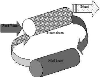
(4) Rubiano, O., Peláez, A. – Dynamic model of the value stream in a power generation …. is a linear relationship between the amount of energy needed and the steam flow, when the energy supplied to the process increases so does the amount of steam generated by the boiler. Figures 1 and 2 show the schematic diagram of a boiler with coal feed. The boiler is made up of basically two components, the tubes where the evaporation of the water takes place and the. boiler’s furnace. While the coal is burned over the stoker grate, the big ashes or boiler slag fall into the ash handling system, the smaller ones or fly ash flow out with the combustion gases. The air used up in the combustion is introduced by the forced draft fan; the induced draft fan takes out the combustion stack gases. The water is supplied with high pressure pumps that force the water into the boiler drum.. Figure 1. Schematic diagram of a boiler with coal feed and grate stoker.. Figure 2. Schematic Diagram of a boiler, mud drum and steam drum.. 94.

(5) Heurística 16, Noviembre 2009, p.91-104. When coal is fed to a combustion process the mass transfer law applies to the original components and its transformation, i.e. the amount of the chemical element carbon in the fuel. There is a linear relationship between the fuel feed rate and the amount of ashes and gases that leave the process. In order to calculate the energy balance, the mass balance must be ready first. There is a conceptual difference between these two calculations. To develop the mass balance it is not necessary to understand how the process takes place, because regardless of the process’s outcome the chemical species that go in the control volume are the same that come out of the control volume plus what accumulates inside of it. It is a different matter to calculate the heat balance because the amount of energy generated throughout the process depends on the resulting chemical components of the combustion reaction. For example, carbon dioxide (CO2) generates a lot more energy per unit mass than carbon monoxide (CO) does according to the following reactions:. 4.2.. . C+O2=CO2 (14.093 BTU/lb fuel).. . 2C+O2=2(CO) (3.950 BTU/lb fuel).. . 2CO+O2=2(CO2) (4.347 BTU/lb fuel).. Assumptions and principles that govern the model. The following assumptions are made in order to model the mass and the energy balance: . . According to the mass conservation law the amount of matter that goes into the control volume is the same that accumulates in the control volume plus the one that comes out of it. There is no water blow down in the boiler.. . The combustion process and steam generation take place in steady state conditions, this means that the boiler is not starting up nor shutting down.. . Even though the steam generation is a deterministic variable and as such can have different values, this variable is defined as a goal to be reached in the simulation.. . The first and second law of thermodynamics is taken into account in the model.. . The notation for the chemical compounds related to the process is a fuel ratio, i.e. for the Carbon Dioxide (CO2) it would be kg.. . CO2/ton of coal. It is assumed that the composition of the combustion compounds is constant and this is an established value determined by chemical analysis.. . During the combustion there is excess Oxygen fed and thus the flue gases are free of Carbon Monoxide (CO). Dry air does not provide energy to the control volume. The amount of air is constant, and so is the ratio of the dry flue gases to the coal fed into the boiler.. . The time unit is a day, all of the units in the model are SI (International System of Units).. . The amount of coal fed into the process is a random variable, it is then supplied to the boiler as a coal rate.. 4.3.. Combustion Reaction Model. Table 1 describes the model variables and equations. Table 2 describes the model’s parameters. To simplify the model it was assumed that the concentration of sulfur, hydrogen and oxygen in the fuel is so low that these compounds can be discarded from the analysis.. 95.

(6) Rubiano, O., Peláez, A. – Dynamic model of the value stream in a power generation …. Table 1. Model Variable.. 96. Variable Name. Description. Equation. Energy in the Control Volume. Difference between the fuel’s energy and the energy that is lost in the flue gases. ∫(Energy Rate in-Energy Rate out-Energy Losses). Energy Rate in. Energy flow per unit of time that goes into the control volume. (Coal Energy + Water Energy in) x Coal Feed Rate. Coal Energy. Amount of energy that goes into the control volume. Conversion Factor (lb/ton) x Calorific Value of Coal x Conversion Factor (BTUkJ). Coal Feed Rate. Coal Flow. Coal Consumption in the Boiler/time. Water Energy in. Water vapor energy flow per ton of coal that goes into the control volume. kg Water/ton of coal x Water molecular weight x Specific Heat of Water @ 303.15 K. Energy Losses. Energy Losses. ((Delta in temperature of flue gases x kg Dry Flue Gases/ton of Coal x Specific Heat of the Flue Gases) + ((Energy flow out dregs )) + Water Energy out x Coal Feed Rate + Additional Energy Losses. Energy flow out dregs. Energy flow that is lost in dregs. Specific heat of dregs x kg dregs/ton of coal. kg Dry flue gases/ton of coal. Amount of flue gases that come out of the control volumen. kg Carbon Dioxide/ton of Coal x Factor Carbon Dioxide + kg Nitrogen/ton of Coal x Factor Nitrogen+ kg Oxygen/ton of Coal x Factor Oxygen. Water Energy out. Energy per ton of coal in the steam that comes out of the control volumen. kg Water/ton of Coal x Molecular Weight of Water x Specific Heat of Water @ 493.706 K. Delta in temperature of the flue gases. Temperature difference between the combustion gases and the environment’s temperature. Temperature of the gases that come out of the boiler - Temperature of the gases that go into the boiler. Energy Rate out. Energy Available for steam generation. Energy Rate in – Energy Losses. Additional Energy Losses. Losses due to radiation. 0.07*Energy Rate in.

(7) Heurística 16, Noviembre 2009, p.91-104. Table 2. Combustion Model Parameters.. 4.4.. Parameter Name. Description. Molecular Weight of Water. Grams of water/molecule of water. Specific Heat of Water. Amount of energy in the water, depends on its thermodynamic state. kg water/ton of coal. Amount of water that goes into the control volume. Initial Ash Concentration. Amount of ash content in the coal when the simulation starts. kg of dregs/ton of coal. Amount of dregs that come out of the control volume. Specific Heat of dregs. Dregs’ capacity to provide energy. Temperature of the gases that go into the boiler’s furnace. Temperature inside the furnace of the boiler. Specific Heat of the Flue Gases. Specific Heat of the Flue Gases. kg Carbon Dioxide/ton of coal. Amount of Carbon Dioxide (CO2) gases that come out of the control volume. kg Nitrogen/ton of coal. Amount of Nitrogen (N2) gases that come out of the control volume. kg Oxygen/ton of coal. Amount of Oxygen (O2) gases that come out of the control volume. Temperature of the gases that come out of the boiler. Temperature of the gases that exit the boiler’s furnace. Mass balance and energy balance of the steam generation system. Basic assumptions. . The main objective of this project is to study the influence of the spontaneous reaction of coal over the fuel inventory and the combustion process.. Table 4 describes the parameters of the steam model.. . The calorific and quality characteristics are known, fixed values.. 5.. . The coal’s consumption is a random variable that displays an uniform distribution behavior.. Assumptions. . The ash concentration is calculated with an empirical equation.. The value stream structure of this research includes the coal stock yard and the fuel conveying system.. Value stream model variables are described on table 5.. Table 3 describes the variables and equations of the model.. Value Stream Modeling in the Pilot Plant. 97.

(8) Rubiano, O., Peláez, A. – Dynamic model of the value stream in a power generation …. Table 3. Steam Model Variables.. Variable Name. Description. Saturated Steam. Energy flow that goes into the control volume. Superheated Steam. Energy flow that comes out of the control volume. Energy Goal. Energy Discrepancy. Equation Steam Rate x (1/Conversion (lb-kg)) x (Conversion (hours/day)) x Saturated Enthalpy Steam Rate x (1/"Conversion (lb-kg)") x "Conversion (hours/day)" x Superheated Enthalpy. Amount of energy neccessary to achive the desired steam flow Amount of additional energy necessary to achieve the desired steam flow. Factor Factor Steam Factor Factor Steam. Superheated Steam-Saturated Steam. Energy Goal-Energy Rate out. Table 4. Parameters of the Steam Model.. Parameter Name. Description. Steam rate. Steam generated in the boiler. Saturated Steam Enthalpy. Saturated Steam energy. Superheated Steam Enthalpy. Superheated Steam energy. Table 5. Model Variable.. Variable Name. Description. Equation. Tons of Stored Coal. The plant’s fuel is stored in this facility. ∫ Fuel Consumption. Fuel Discrepancy. Coal flow necessary to compensate the energy requirements of the boiler. Energy Discrepancy/(Conversion Factor (lb/ton) x Calorific Value of Coal x Conversion Factor (BTU-kJ)). Fuel Consumption. Coal flow. RANDOM UNIFORM(200,300,350) + Fuel Discrepancy. Calorific Value of Coal. Fuel’s Capacity to provide energy. (144.9*Carbon Concentration+2664)*Factor. Carbon concentration. Carbon, chemical element’s concentration of the fuel. (100-Ash Concentration - ((Factor Dregs) x (kg Dregs/ton of Coal)/10)). Ash Concentration. Amount of ash generated by coal’s spontaneous combustion Empirical equation.. 0.1612*Simulation Time^2+0.4583*Simulation Ash Concentration. Coal consumption in the boiler. Coal accumulation in the boiler. ∫ Fuel consumption. Simulation Time. Simulation Runtime. Factor Day*Simulation Factor. 98. Time+Initial.

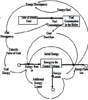
(9) Heurística 16, Noviembre 2009, p.91-104. Figure 3 illustrates the casual diagram where the relationship between the different type of variables is shown. Likewise, figure 3 shows the cause and effect relationships that establish the way the variables in the model need to be calculated. The causal diagram contains two feedback loops that determine the system’s behavior. The positive feedback loop shown in the upper part of the diagram reinforces the. relationship established between the coal feed rate and the generation of energy, the more energy that is needed means more coal necessary to be supplied to the process. The negative feedback loop shown in the lower part of the casual diagram characterizes this model as a “goal seeker” where the system displays a trend to estabilize itself. Figure 4 shows the Forrester diagram of the model.. Figure 3 Causal Loop Diagram of the system.. Figure 4. Stock and Flow Diagram of the system.. 99.

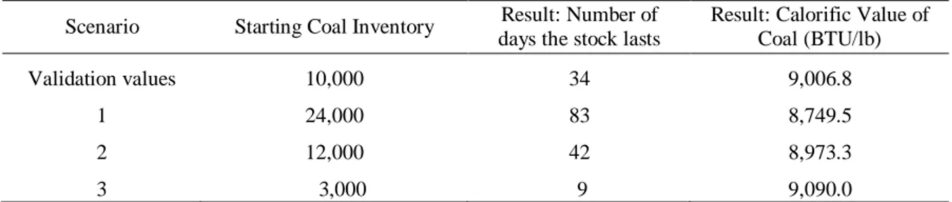
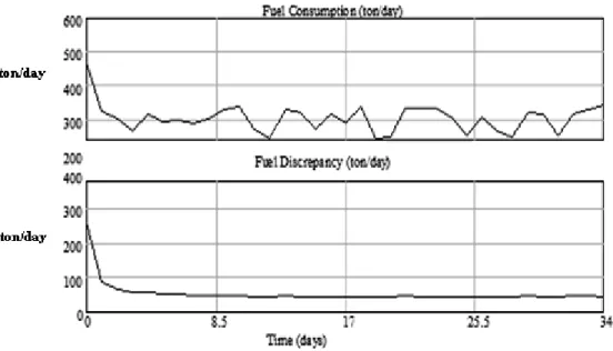
(10) Rubiano, O., Peláez, A. – Dynamic model of the value stream in a power generation …. 6.. Discussion and Results. 6.1.. Validation of the behaviour patterns for the main model variables. Recent data shows that the coal fed into the boiler has an average calorific value of 11,347.52 BTU/lb, 17.51% of ashes and a power generation ratio of 14,345.3 pounds of steam/ton of coal. The average coal stock was 10,000 tons per month, and the steam rate of the boiler was 220,987 pounds of steam/hour. The simulation runtime span was 34 days and had a starting coal stock of 10,000 tons, and a fixed steam rate, these inputs resulted in a calorific value of 9,022.28 BTU/lb and 18.1% ash content. The heat transfer efficiency of the boiler was close to 73%. Riley, the boiler’s manufacturer did an engineering study in 1991 to calculate the process’s efficiency. In this study the coal had a calorific value of 9,559 BTU/lb and a 13.54% ash content. The efficiency of the heat transfer process was 75.12%. The steam rate per ton of coal ratio that Riley calculated in the study was 18,000. The heat transfer efficiency that the simulation calculated was very similar to the result that Riley reported on the engineering study. The percent difference between the model’s efficiency and Riley’s study was 2%. It is to be noted that the calorific capacity of the recent data is 20% less. than the one reported on the engineering study.As a conclusion, it can be stated that the model is representative of the value stream system studied.. 6.2.. Using the model. The main objective of the development of the model is to study the connection between the process and the value stream. On every scenario the steam rate is fixed at 220,000 pounds/hour and the starting inventory has a set value also. During the simulation run time span the coal’s calorific value is calculated. This result indicates how much the fuel has deteriorated while it has been stored. Table 6 shows for each scenario, the calorific capacity of the coal at the end of the simulation runtime. At the beginning of the simulation the fuel’s calorific capacity is 9,112.05 BTU/lb. Table 7 shows the ash content. At the beginning of each simulation run, the ash content is 17.5%. The lower coal ash value matches the smallest amount of starting coal inventory (3,000 tons), and the larger coal ash value matches the biggest starting coal inventory (24,000 tons). Figure 5 shows the behavior of the variable coal feed rate, for a starting fuel inventory of 10,000 tons of coal and a 34 day run. Its behavior is mainly random, and this fits with the actual fuel feed procedure.. Table 6. Calorific Capacity of the coal after running the simulation.. Scenario. Starting Coal Inventory. Result: Number of days the stock lasts. Result: Calorific Value of Coal (BTU/lb). Validation values. 10,000. 34. 9,006.8. 1. 24,000. 83. 8,749.5. 2. 12,000. 42. 8,973.3. 3. 3,000. 9. 9,090.0. Table 7. Ash content in the boiler after running the simulation.. 100. Scenario. Starting Coal Inventory. Ash Content (%). 1 2 3. 24,000 12,000 3,000. 20.0 18.4 17.6.

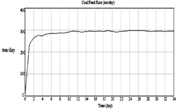
(11) Heurística 16, Noviembre 2009, p.91-104. Figure 5. Coal Consumption in the boiler and fuel discrepancy.. The variable fuel discrepancy fluctuates between 40 and 50 tons of additional coal per day, in order to compensate for the process’s inefficiencies. At the beginning of the simulation the disparity is large, but as the simulation runs the variable tends to stabilize. This behavior is accounted for the negative feedback loop that makes up the model’s structure. A similar behaviour is displayed by the variable Energy Discrepancy. Figure 6 shows how the average coal feed rate burned in the boiler tends to an average value of 296 tons/day. With this fuel, the amount of energy produced ranges between 5.5 and 5.6 X 10 EXP 9 kJ/day. This energy flux compensates the fuel’s degradation, shown on Figure 7. The positive feedback loop shown on Figure 4 explains the initial offset of the coal feed rate that compensates the energy requirements of the process due to energy losses. The stability that the variable reaches is explained by the negative feedback loop of the system structure. This feedback loop relates the coal feed rate and the amount of fuel stored with the energy balance of the process.. Figure 8 shows the behavior of the variable that makes up the energy balance. Such a behavior is governed by the positive feedback loop of the causal loop diagram. However, on the long run, the stabilizing effect over the variable is explained by the negative feedback loop. Results show a linear relationship with a small slope relating the fuel’s consumption to the inventory time for these three scenarios (Figure 9). This means that the inventory time has a linear relationship with the initial amount of coal stocked. The linear tendency indicates that the coal’s degradation is influenced by several conditions that also have an effect on the coal’s consumption. If the model runs with initial coal stocks larger than 24,000 tons the relationship between the variables is not linear. In these cases the storage time and its relationship to the amount of coal is still directly proportional. However, in these scenarios doubling the amount of coal stored doesn’t double the time the fuel is available, the relationship is not linear. The coal’s availability increases at a smaller rate compared to its initial inventory.. 101.

(12) Rubiano, O., Peláez, A. – Dynamic model of the value stream in a power generation …. Figure 6. Coal Feed Rate.. Figure 7. Coal’s Degradation.. 102.

(13) Heurística 16, Noviembre 2009, p.91-104. Figure 8. Energy Balance in the Boiler.. Figure 9. Tons of Coal and Storage Time.. 103.

(14) Rubiano, O., Peláez, A. – Dynamic model of the value stream in a power generation …. 7.. Conclusions. Experimental results in coal storage yard. Fuel Processing Technology 59(1):23-34.. In this research, the impact of storage time over coal’s calorific capacity was studied. A contribution of this research was the development of a model that simulates the value stream of steam production in a chemical processing plant. The model was created based upon the casual relationships that determine the fuel’s reactions in the combustion process. The results show the effect of time over the fuel’s calorific capacity in this energy process. Of the coal’s components, elemental Carbon is the main responsible for the fuel’s calorific capacity and its economic value. The calorific capacity loss was related to the degradation rate, as the coal downgrades into ashes on account of spontaneous combustion. The variable, coal feed rate shows that the fuel consumes itself with a uniform behavior. A future development of this study could include an economical analysis of the fuel’s storage time. Further development of this research would consist of studying this issue for a complex value stream of the fuel. A further enhancement of the model would include the coal’s reception rate in the warehouse.. 8.. 1. Ballou, Ronald. 2004. Logística: Administración de la cadena de suministro. Mexico: Prentice Hall. 2. Basil Beamish and Ahmet Arisoy. 2008.. Effect of mineral matter on coal selfheating rate. Fuel 87(1), January:125-130 Bejan, Adrian. 1997. Advanced engineering thermodynamics. United States: John Wiley & Sons. 3. Brooks, Kevin and David Glasser. 1986. A. simplified model of spontaneous combustion in coal stockpiles. Fuel 6(8):1035-1041. 4. Fierro, Vanessa, C. Romero and J. L. Miranda. 1999. Prevention of spontaneous. 104. 6. Hougen, Olaf, Kenneth Watson, y Roland Ragatz. 1982. Principios de los procesos químicos. España: Editorial Reverté. 7. Krishnaswamy, Srinivasan, Robert D. Gunn and Saurabh Bhat. 1996. Low-temperature oxidation of coal. 1. A single particle reaction diffusion model Fuel 75(3):333-343. 8. Pone, Denis, Glenn B. Stracher and Kim A.A. Hein. 2007. The spontaneous combustion. of coal and its by-products in the Witbank and Sasolburg coalfields of South Africa International Journal 72(2):124-140.. of. Coal. Geology. 9. Reklaitis, Gintara y Daniel Schneider. 1989. Balances de Materia y Energía. Mexico: McGraw-Hill. 10. Sipper, Daniel, y Robert Bulfin. 1997. Planeación y control de la producción. México: McGraw-Hill.. References. combustion. 5. Himmelblau, David. 1997. Principios Básicos y Cálculos en Ingeniería Química. México: Prentice Hall.. in. coal. stockpiles:. 11. Smith, Joe, Hendrick Van Ness, Michael Abbott. 2000. Introducción a la termodinámica en Ingeniería Química. México: McGraw-Hill. 12. Smith, Myles and David Glasser. 2005. Spontaneous combustion of carbonaceous stockpiles. Part I: the relative importance of various intrinsic coal properties and properties of the reaction system. Fuel 84(9):1151-1160. 13. Sterman, John. 2000. Business Dynamics:System Thinking and Modeling for a Complex World. United States: McGrawHill..

(15)