Estimating the modal parameters from multiple measurement
setups using a joint state space model
F. Javier Cara , Jesús Juan , Enrique Alarcón
A B S T R A C T
Computing the modal parameters of structural systems often requires processing data from multiple non-simultaneously recorded setups of sensors. These setups share some sensors in common, the so-called reference sensors, which are fixed for all measurements, while the other sensors change their position from one setup to the next. One possibility is to process the setups separately resulting in different modal parameter estimates for each setup. Then, the reference sensors are used to merge or glue the different parts of the mode shapes to obtain global mode shapes, while the natural frequencies and damping ratios are usually averaged. In this paper we present a new state space model that processes all setups at once. The result is that the global mode shapes are obtained automatically, and only a value for the natural frequency and damping ratio of each mode is estimated. We also investigate the estimation of this model using maximum likelihood and the Expectation Maximization algorithm, and apply this technique to simulated and measured data corresponding to different structures.
1. Introduction
The modal analysis of a structural system consists of computing its vibrational modes. The experimental way to estimate these modes requires exciting the system with a measured or known input (for example, with a hammer or a shaker), and then measuring the system output at different degrees of freedom (DOFs) using sensors. When the system refers to large structures like buildings or bridges, to apply a known input (more suitable for laboratory conditions) is usually difficult and expensive, and uncontrolled disturbances are also present during the measurements. This led to the idea of performing the modal analysis using ambient vibrations, that is, the vibrations due to unmeasured inputs like wind, traffic, human action, ground vibrations, etc.
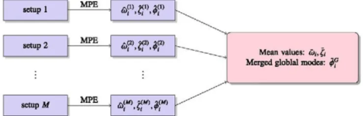
setup 1
Mean values: ¿>¡,£ Merged globlal modes: <f>f
setup M
Fig. 1. Merging M individual partial mode shapes into a global mode shape (the multi-step approach). MPE means modal parameter estimation.
setup 1
setup 2
setup M
Proposed model MPE Estimated parameters C>ul,Vf Estimated parameters
C>ul,Vf
Fig. 2. Estimating the modal parameters processing M setups at the same time (the one-step approach). MPE means modal parameter estimation.
sensors among setups [2]. Since the mode shapes estimated in each setup cannot be scaled in an absolute sense (e.g. to unity modal mass), some sensors have permanent positions because these fixed or reference sensors are needed to glue or merge the mode shapes estimated at each setup (or partial mode shapes) into global mode shapes. The rest of the sensors change their position in the structure from one setup to the next, so different parts of the global mode shapes can be estimated. The algorithms available to estimate or identify the modal parameters from ambient vibration measurements (also known as Operational Modal Analysis or OMA) were originally developed to process the measured data of one setup of sensors [1,3]. That is why it is usual to process separately the data measured in each setup and then merge the partial mode shapes to obtain global ones: the reference sensors are used to combine the different parts of the mode shapes, while the eigenfrequencies and damping ratios are averaged. This way of computing global mode shapes, which can be named as the
multi-step approach, is outlined in Fig. 1. However, some drawbacks can be pointed out:
1. If the number of setups is large, this approach is tiresome, especially if the modes of interest are not well excited and therefore difficult to extract at all the setups [4-6],
2. Since the excitation cannot be controlled or measured, differences in the excitations result in the extraction of spurious
or unphysical modes in some setups while these modes are not found in the other setups [4-6],
3. It is not easy to pair the corresponding mode at each setup, especially when there are modes with closely spaced natural
frequencies or with similar mode shapes at the reference DOFs [4-6],
4. A lot of effort has to be made to properly merge the different parts of the mode shapes estimated in each setup, for example in a least square sense [7],
On the other hand, there is an increasing interest to process all setups at the same time because the global mode shapes are obtained automatically (the one-step approach, in contrast to the multi-step one, shown in Fig. 2): in Ref. [8]
a frequency-domain maximum likelihood identification technique was used for the modal parameter estimation. A comparison was made between a non-parametric and a parametric approach, where the unwanted non-stationary
effects are removed respectively before and after the system identification step; in Refs. [9-11] the Stochastic Subspace
Identification (SSI) method was adapted to handle these kinds of problems. However, it is necessary to normalize the data of the different setups before to apply the algorithms because the unmeasured background excitation of each setup might be different. Finally, some of these techniques were analyzed and compared in Refs. [2,12,13],
In this work we propose a new state space model to manage multiple setups of sensors and ambient vibrations. The model, described in detail in Section 2.1, belongs to the one-step approach (Fig. 2). Its main properties are:
The drawbacks described for the multi-step approach are overcome: 1. All setups are processed at the same time.
2. The model extracts the parameters that are common to the setups. 3. Pairing modes among setups is not needed.
4. Global mode shapes are obtained directly, without further treatment.
• The model can be used with the known scheme of permanent-moving sensors, where permanent sensors do not change their position from setup to setup. But the model allows to use setups without permanent sensors. The only requirement is that each setup shares the position of some sensors with at least another setup (the overlapped sensors). The number of overlapped sensors can be different from one setup to the next.
We propose to estimate the model by the maximum likelihood method using the Expectation Maximization (EM)
algorithm. The name EM was given by Dempster et al. [14], who presented the general formulation of the algorithm,
established its basic properties and provided many examples and applications. Since then, it has been profusely used in many problems: engineering, psychometry, econometrics, epidemiology, genetics, astronomy, etc. A review of the
applications of the EM algorithm in many different contexts can be found in the monographs of Little and Rubin [15]
and McLachlan and Krishnam [16],
For the state space model, the EM algorithm was developed by Shumway and Stoffer in 1982 [17]. The method has been
applied to a variety of problems: estimation of dynamic unobserved component models [18], estimation of covariance
parameters in a state space model [19], non-linear system identification [20], speech recognition [21], operational modal analysis [22] and many others.
Section 3 describes how the EM algorithm is extended to estimate the proposed model. In particular, the log-likelihood function for multiple setups and the equations obtained in the Expectation and the Maximization steps are derived. Since the model has not been used before, these equations are presented in this work for the first time.
The method has been tested in a series of examples. In Section 4 we have applied the method to simulated data that
allows to compare the estimated parameters with their theoretical values. We have studied the case of reference-moving sensors and the case of overlapped sensors. We have also compared the proposed method with the traditional multi-step approach.
In Section 5, we have used experimental data from a footbridge. In total, thirteen setups were recorded: each setup comprised three permanent triaxial stations and four mobile triaxial stations (21 recorded channels each setup). This real structure with a high number of setups and measured DOFs shows the applicability and advantages of the method.
Finally, in Section 6 the method has been applied to experimental data measured at a building. In this case, the technique of permanent-moving sensors cannot be used because the data were not recorded using fixed sensors. However, the proposed method is capable of estimating the modal parameters in this structure as well.
2. The state space model
2.2. The proposed state space model
Consider a linear, time invariant structural system. In this system we measure M different data series for the input ut and
the output yt. For simplicity, we are going to consider that all the records have the same length, N. The data can be
represented by
^ = { ) M V - - » 3 # } , r = l , 2 , . . . , M , (1)
U$ = {u(p,u<p,...,u(N}, r=\,2,...,M, (2)
where Y$ e Rn°T is the measured output vector for record r, and Uff e Rnir is the measured input vector for record r. Thus, nor
and nir are the number of outputs and inputs for record r. In principle, we consider that the inputs can be applied at different
points from record to record. We also consider that the outputs can be measured at different places. The state space model we can use for these data is
v(r) -.A^p + B^pWp, (3a)
y'f^C'^x'p+D^u'p+v'p,
r = \,2,...,M, (3b)
where t denotes the time instant, of a total number N, measured with constant sampling time At; xf} e U"s is the state vector
for record r; ns is the order of the state vector, which is constant to all the records; A e R"sX"s is the transition state matrix
describing the dynamics of the system; B(r> e un*'An* is the input matrix; C(r> e un"'xn' is the output matrix, which is describing
how the internal state is transferred to the output measurements yf}; D(r> e un°T'x-n<r is the direct transmission matrix.
The noise vectors comprise unmeasurable vector signals: wP e Rn* is the process noise due to disturbances and modelling
discrepancies, while vp} e U"" is the measurement noise due to sensor inaccuracy.
It is important to note that matrix A is constant and equal for all records because the system is assumed to be time invariant, does not change from the first record to the last record. On the other hand, B(r> and D(r> are record-depending
because the system input can be different from record to record. C(r> is also record-depending because the sensor placement
In the case of output-only testing, only the response of the structure is measured, while the input sequences 1/}J unmeasured. Thus, Eq. (3) results in
x'fl^Ax'p+w'p, (4a)
yf) = C(r>xf)+vf),
r=\,2,...,M. (4b)
We propose to write this model as
x'fl^Ax'p+w'p, (5a)
yP=l^CxP + vP,
r=\,2,...,M, (5b)
where Ce un°'xn* is the global output matrix, corresponding to all DOFs where the output has been measured; n0 is the
number of different DOFs where the output has been measured; L(r> e Rn°'xn° is a location or selection matrix formed by ones
and zeros verifying C<r) = L(r>C; so if we define a vector with all the different DOFs that have been measured in the structure,
called the global list of measured DOFs or yf^ e R"°xl, the location matrices L(r> need to verify yf> =L(r>yf\ The location
matrices are known for each setup r.
The state space model given by Eq. (5) is the model we are going to use in this work. We assume that the noise processes wf) and vP are independent white noise sequences with w(tr)^N(0, Q}r>) and vP^*N(0,R<T)). We also need an initial condition
for the difference equation (5a): we shall assume that x(p is a Gaussian random variable of known mean ¡Jp and known
covariance ¿p. Further, we shall assume that x(p is independent of wp} and vp} for any t.
Therefore, the unknown parameters of the model (5) are
9 = {A,C,Q(r\R(r\t¿<o\z<p}, r = l , 2 , . . . , M . (6)
2.2. The state space model and modal parameters
Modal parameters are computed from the parameters of the state space model, in particular from matrices A and C (see [1]). It is usual to express thejth eigenvalue of A as
X¡ = exp -Zja>i±ia>iSJ\-i:f\^t\, (7)
where At is the time step. Therefore
a>¡ = — , ( 8 )
1 At ' y '
-Real[ln(a,Q]
Q¡~ cojAt • ( 9 J
If proportional damping is admitted, w¡ is the undamped natural frequency and Q is the damping ratio. Thejth mode shape <pj e Rn° evaluated at sensor locations can be obtained using the following expression:
4>j = CVj, (10)
where \¡/¡ is the eigenvector corresponding to X¡.
3. Maximum likelihood estimation: EM algorithm
To estimate the parameters of the state space model (5), we propose to use maximum likelihood estimation (MLE) with a
maximization procedure based on the Expectation Maximization algorithm. The EM algorithm is a general-purpose method for MLE [14], and the first applications to estimate the state space model can be found in the works of Shumway and Stoffer
[17,23]. The performance of the EM algorithm for OMA analysis was tested in [22]. The algorithm is simple to apply since at each iteration the optimal solution for the unknown parameters can be obtained from explicit formulas.
3.1. Computing the likelihood function
Let the observed outputs Y(p = {y(p,y(2,-.-,y(p) and the states XÍQ = {xip,x(p,...,x(p). The density function for one
individual record is given by (see [22])
N N
where under Gaussian assumption
K ^ I Y C ) A - 1 ovn^-l/vC) 4v« ^,,n(rK-l/v(r)_4v(r)
Thus, if we consider M independent setups, the joint density function fa(XN, YN) will be the product of individual ones M
f
e(x
N,Y
N)= n/
e«(xK
>)- a 2)
r = 1
The complete data likelihood is defined by LxNyN(9) =fs(XN, YN). In practice the log-likelihood is used, so information is
combined by addition and it can be written as a sum of the log-likelihood of each individual record:
M
ixN,YN(0) = logLxN,yN(0)= 2 /x«y«(0«). (13)
r = 1 N' N
The log-likelihood of record r can be written as the sum of three uncoupled functions
¡ xM ? (*<r)) = ~\ ['i U M ) + b ( ^ Q( r )) +'3 ( C , ü « ) l , (14)
N ' N
where ignoring constants are
i, ($, 4
r )) = i o g i 4
r )i+(4
r >-^E)
r))
T(4
r>)"' (4
r>- ^
r >) , a 5)
(V
i
2(Aa
<r))=Niogia«i+ 2 (xf-Axf^^a^-^x^-^,), ae)
t = l
JV
i3(C,R<r)) = Nlog|R<r)|+ 2 (yP-LVQÍpfíRPrWP-lPCx/P)- (17)
t = i
If we did have the observed vectors Y^ and the states X$, we could easily obtain the MLEs of the parameters 9 (for example, using the results from multivariate normal theory). But the states are unknown (in fact, the states are unobserved quantities). The EM algorithm gives us an iterative method for finding the MLEs of 9 using only the observed vectors Y$, by
successively maximizing the conditional expectation of the complete data likelihood (13). Two steps must be repeated
iteratively:
• Expectation step: To compute the expected value of the log-likelihood (13), E[1XNJN(9)\YN, 9¡\
• Maximization step: To maximize E[IXN,YN(9)\YN,9¡] with respect to the parameters 9.
3.2. E-step: expectation step
The expected value of log-likelihood (13) given the measured data and a value for the parameters 9¡ is
M
E[IXN,YN(9)\YN,9J]= 2 E [ /X„ ^ ( ^ ) | y « i f ]
M
= 2 ( E l h ^ U Í ^ I ^ V f l + E f c í A a ^ í l ^ ^ f l + E f c í C ^ ^ i y ^ ^ f ] ) (18) r = 1
Operating it is obtained:
E [ /1^ , 4r))| y í V f ] = l n | 4r )l + t r ( ( 4rV n Cr ) + ( ^< r )- ^)) ( ^ r - ^T] ) > (19)
Efe (A, Q.<f>)\Y'tt, éf> ] = N log | Q.<f> | + tr((Q(r)) - ' [Sg - S%AT -A$¡ +A^>AT]\ (20)
where tr(») is the matrix trace operator and
Sg= Í(P?M+x!tM<x!t#>)
T), S«= £ ( ^ ? + « «T) , (22)
t = i t = i
SS= Z ( ^ , + ^ ( x « ' ? )
T) , Sg = (S«)'-, (23)
t = i
(V
$ = 2 y
t(xf'
(r))
T, s« = (s«)
T. (24)
t = i (V
sg= 2 yf^y, (25)
t=iwhere it has been taken as follows:
x^(r) = E[x(p\Y^,0fl (26)
ff(r) = E[(xf -xf-^Xxf -xf'( r ))|y«, é f ], (27)
P ™ = E[(xf - x f « ) (x« , - x ™ ) < , é f ]. (28)
These last terms, Eqs. (26)-(28), are computed using the Kalman Filter and the Kalman Smoother (see [22]).
3.3. M-step: maximization step
Maximizing E[lXNjN(ff)\YN,9j] with respect to the parameters 9 constitutes the M-step. This is the strong point of the EM
algorithm because the maximum values, obtained equating to zero the corresponding derivatives (see Appendix A), are
obtained from explicit formulas.
• Maximizing E[Ji(^r\¿#))lyN>éf)] r e s u l t s i n
ftf=^\ (29)
4
r )= P T . (30)
• Taking the derivative of E[/2(A, QP)\Y^, 9(p] with respect to A and equating to zero we obtain
M M
2((a
<r))-Ms«)= 2((Q
<r>r
1s2) (3i)
r = 1 r = 1
Taking the vector operator of a matrix vec(»), we can write the linear system of equations to compute A M M
2 (Sti ® (Q.(r))-')vec(A)= 2 v e c í í a ^ ) -1^ ) (32)
r = 1 r = 1
where <s> is the Kronecker product. This equation can be solved because 25'Li (S^ <s> (Q(r))_1) is non-singular. Thus
vec(A) = f I (S« ® (Q(r))"!)) f vec((Q(r)) - ' s g ) (33)
\r = 1 / r = 1
• Taking the derivative ofE[l2(A,QP)\Y<$,ef)] with respect to Q.<r) we obtain
a
<r)=¿(sS-sSA
T-As«
+As«A
T). (34)
• In a similar way, the maximum of E[/3(C,R<r))|y^Vjr>] is attained at
vec(C) = ( 2 (Sg ® ((L«) W
1!
0 0) ) 2 v e c C W V
1^ ) (35)
\r = 1 / r = 1
The two steps, expectation and maximization, have to be repeated iteratively until the likelihood is maximized. The overall method can be summarized as follows:
Initialize the procedure 0 = 0 ) selecting starting values for the parameters 90 = (A0,Co,Q$\^\Poo>Z$o) a nd a s t 0P
tolerance Sadm.
Repeat
= (A, C, Q ^ i ^ , ^ , ! ^ ) using (29)-(36).
1. Perform the E-Step. Apply the Kalman filter and smoother (see [22]) to obtain the expected values xf<r), Pf<r), and P^f2-¡ using 9¡ as data. Use them to compute the matrices S^, S^ and S%[ given by (22)-(24).
2
Perform the M-Step. Update the parameters 9j+ ^
3- Compute the likelihood E[/XN,YN(6»)|YN, ^_/ +1] using (18).
4. Compute the actual tolerance
|E[txw,yw(fl)|yN,gj+i]-E[tXw,yw(fl)|yN,gJI (37)
(a) If S > Sadm, perform a new iteration with 0¡+-l as the value of the parameters.
(b) If S<Sadm, stop the iterations. The estimate is 9j+-¡.
3.5. Starting values for the EM algorithm
The selection of the starting point for the EM algorithm is not easy for models like (5). In our opinion, it is advisable that the starting point meets two properties: first, it is built fast and easy; and second, it has to take advantage of the information provided by the data. We think a good alternative is to use the parameters estimated with another method (for example, SSI) to build the starting point. This approach can be used here applying SSI to one setup and then using the result as starting point for all the setups. We propose to build the starting point 90 = (Ao,Co,Qo),^o)'/'oo''£oo) a s follows:
First, to apply the SSI algorithm to one of the setups, setup s, obtaining A^¡, d^¡, Q_% and R^¡.
A0 =A^i- We take advantage of the information given by the eigenvalues ofA^. These eigenvalues may be influenced by
the particular position of the sensors in setup s, but their information is useful to the EM algorithm to convergence to the right solution.
C0 is constructed so that the product Úr)C0 is equal to the first nor rows of C §r This condition gives us an idea of the
relation between the states given by A0 and the outputs. Again, this is only valid for setup s, but it is enough for a
starting point.
Q¡p = ()§, for all r. The result is a positive definite matrix (this is important for the EM), and it is a good approximation to the rest of the covariance matrices.
R(p is the first nc
fip0 and Z(p0 are taken matrices of zeros.
rows and columns of R^¡. It is another positive definite matrix and adequate for the outputs.
Note that this approach to build the initial point needs SSI to be applied to the setup with the larger number of measured points (the larger nor).
4. Numerical example 1: simulated data
4.1. Description of the data
An eight DOF simulated structure is used in this section to validate the proposed method. It consists in 8 masses and 9
springs and dash-pots (Fig. 3(a)), and the values chosen for the mass matrix M, the damping matrix V and the stiffness
matrix K are the following:
2400 -1600 0 0 0 0 0 0
-1600 4000 -2400 0 0 0 0 0
0 -2400 5600 -3200 0 0 0 0
0 0 -3200 7200 -4000 0 0 0
0 0 0 -4000 8800 -4800 0 0
0 0 0 0 -4800 10 400 -5600 0
0 0 0 0 0 -5600 12 000 -6400
0 0 0 0 0 0 -6400 13 600
TÍW- "iiTWP- ^2TMF mJUT mJUT^
m5jfiP~
lki,Ci K2,C2 K3, C3 kn, Cu k¡,C¡ Kfr, C(, ki,ci kg,cg k9,c9 I
0 0 t r o 0 0 0 0 t r o 0 0 0 0 0 0
Mode 1: f = 2.94 Hz, i; =2.00%. Mode 2: f = 5.87 Hz, i; =1.24%.
Mode 7: f = 19.54 Hz, i; =1.35%.
0 - E ¡
-1
0 2 4 6 Mode4:f = 11.19 Hz, £ =1.10%.
f H ^ oU^
0 2 4 6 Mode 6: f = 16.52 Hz, i; =1.23%.
-^•er
0 2 4 6 Mode 8: f = 23.12 Hz, i; =1.50%. 1
o - El-3—a—B^~E Í'
-1
Y
0 2 4 6 8 0 2 4 6 8 Fig. 3. (a) Model of the simulated structure, (b) Natural frequencies, damping ratios and mode shapes of the simulated structure.
M is equal to the identity matrix with eight rows and columns, and V is built assuming Rayleigh damping by means of
£> = 0.68OM +1.743 x 10~4K; (N s/m). (39)
The natural frequencies, mode shapes and damping ratios corresponding to matrices M, V and K, are presented in
Fig. 3(b).
The output signals have been obtained using:
• The acceleration of the eight DOFs has been generated three times in order to simulate three different tests.
• The input in each test is Gaussian white noise with zero mean and variances 1, 4 and 9 for each one (the excitation level is different for each setup). These inputs have been applied to all the DOFs. The objective is to excite all the modes, that is why the inputs are white noise and have been applied to all DOFs.
• Sampling frequency fs = 50 Hz. Total duration of signals, 100 s (5000 time steps).
• The observed value is the sum of the structure response and a sensor Gaussian noise with variance equal to the 20% of the largest acceleration response variance.
4.2. Proposed method with permanent-moving sensors
First we are going to apply the method considering permanent-moving sensors, that is, all the setups have a certain number of sensors located at the same place (the permanent sensors) and the rest are moving sensors. This strategy is
widely used nowadays to estimate the modes of large structures (see for example [2,10,12,13]). We have simulated the
following three setups of sensors:
That is, we have considered masses 1 and 2 as permanent pools, and the rest are moving pools. Besides, we have considered different number of moving sensors in each setup: three, two and one respectively.
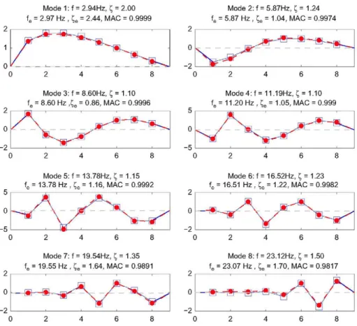
The location matrices for this case are built now. First, we define the global list of measured DOFs , yf\ and the measured DOF at each setup
„<c).
" ¿ T i . c "
<?2,t
" Q i . t " 9 3 , t
<Í2,t "<7i,t"
"9i,r
Q.4,t; W =
<Í3,t ; y(? = Q.2,t$6,t
;
y?
=
92,tQ.4,t Q.2,t
$6,t
94,t qs.t
Qs,t
A'.
h,tQi,t
Qs.t
(40)
where qkt is the acceleration of mass k at time instant t. The following relationships must be verified:
yCl) = L0)yf\ yf> = L(2)yf^ y(3) = ¿0)3,(0. (41)
Thus
i d ) .
L®:
1 0 0 0 0 0 0 0 0 1 0 0 0 0 0 0 0 0 1 0 0 0 0 0 0 0 0 1 0 0 0 0 0 0 0 0 1 0 0 0
1 0 0 0 0 0 0 0 0 1 0 0 0 0 0 0 0 0 0 0 0 0 0 1
r ( 2 ) .
1 0 0 0 0 0 0 0 0 1 0 0 0 0 0 0 0 0 0 0 0 1 0 0 0 0 0 0 0 0 1 0
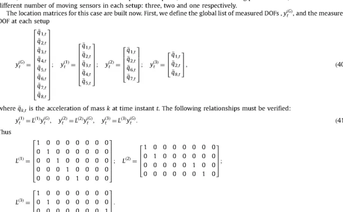
The proposed method has been applied to the simulated data obtaining the results shown in Fig. 4 (the starting point
was built applying SSI to record 1 according to Section 3.5). The natural frequencies and mode shapes are estimated with
precision; the damping ratios have more bias, even when using simulated data. This variability of damping ratios is not a drawback of the EM algorithm, but it is present in greater or lesser extent in all
the identification methods (see [25] for a comparative analysis of damping ratios estimated using different approaches).
4.3. Multi-step approach
Fig. 4 shows that the values obtained using the proposed method with the simulated data are good. An important issue is the comparison of these results with the traditional scheme of processing each setup separately and then merge the partial mode shapes (the multi-step approach, in contrast to the proposed method which can be considered as a one-step
approach). We have estimated the modal parameters from the setups 1, 2 and 3 used in Section 4.2 by means of the SSI
algorithm under a state space order ns= 16 (the theoretic order). Since the natural frequencies are quite separated, it is easy
to identify the corresponding modes in each setup. Then, mean frequencies and mean damping ratios of each mode can be
computed, and the global mode shapes can be easily merged. Table 1 shows the obtained results.
In general terms, the natural frequencies estimated by SSI in the three setups are very similar to the theoretical ones. The main deviations are observed in mode number 8, although it is a small one: theoretical=23.12 Hz, estimated in setup 1 =24.08 Hz (5.25%). On the contrary, the variability in the estimated damping ratios is higher: for mode 8 (estimated worse mode), the theoretical value is 1.50, and the values estimated for setups 1, 2 and 3 are 2.62,1.51 and 1.86 respectively (mean value equal to 2.00). Finally, MAC values between the merged modal shapes and the theoretical ones are very good for modes 1-5, not so good for modes 6 and 7, and bad for mode 8.
The natural frequencies and damping ratios estimated by the proposed one-step method are very similar to the mean values of the SSI. However, the MAC values corresponding to the one-step approach are very good for all the modes, even for mode 8 (MAC = 0.9817).
4.4. Proposed method with overlapped sensors
We show now that the method can be used with more general setups of sensors, for example with setups without permanent sensors. As indicated in the Introduction, the only requirement is that each setup shares the position of some sensors with, at least, another setup (the overlapped sensors). In this example we define:
Mode 1:f = 2.94Hz, £ = 2.00 f6 = 2.97 Hz , t,e = 2.44, MAC = 0.9999
Mode 2: f = 5.87Hz, £ = 1.24 f6 = 5.87 Hz , ¡;e = 1.04, MAC = 0.9974
Mode 3: f = 8.60Hz, C| = 1.10 f6 = 8.60 Hz ,¡;e = 0.86, MAC = 0.9996
Mode4:f = 11.19Hz, £ = 1.10 f6 = 11.20 Hz , ¡;e = 1.05, MAC = 0.999
w
Mode5:f = 13.78Hz, £ = 1.15 f6 = 13.78 Hz , ¡;e = 1.16, MAC = 0.9992
Mode6:f = 16.52Hz, £ = 1.23 f6 = 16.51 Hz , ¡;e = 1.22, MAC = 0.9982
Mode7:f = 19.54Hz, £ = 1.35 f6 = 19.55 Hz , ¡;e = 1.64, MAC = 0.9891
--H—S-Mode 8: f = 23.12Hz, £ = 1.50 f6 = 23.07 Hz , ¡;e = 1.70, MAC = 0.9817
o
—
f f i a
-- 2 I •— 0 2
--a-fl^^y^
Fig. 4. Theoretical modes ( • ) versus estimated modes (•) using the proposed method and considering permanent-moving sensors. fe and fe stand for estimated frequency and damping ratio respectively. MAC is computed between theoretical mode shapes and estimated mode shapes.
Table 1
Natural frequencies and damping ratios estimated from the simulated data: SSI(k) stands for the values estimated applying the SSI algorithm to setup k(ns — 16); "SSI mean" is the mean of the values estimated with SSI; EM stands for the values obtained using the proposed method (permanent-moving sensors); MAC values are computed between estimated mode shapes and the theoretical ones.
Modal parameters Mode number
1 2 3 4 5 6 7 8
Frequencies (Hz) 2.94 5.87 8.60 11.19 13.78 16.52 19.54 23.12 Theoretical 2.95 5.86 8.60 11.25 13.75 16.54 19.54 24.08 SSI(l) 2.96 5.87 8.63 11.19 13.80 16.52 19.72 22.88 SSI(2) 2.96 5.85 8.60 11.18 13.79 16.55 19.63 23.14 SSI(3) 2.96 5.86 8.61 11.21 13.78 16.54 19.63 23.37 SSI mean 2.97 5.87 8.60 11.20 13.78 16.51 19.55 23.07 EM Damping ratios (%) 2.00 1.24 1.10 1.10 1.15 1.23 1.35 1.50 Theoretical
3.32 1.10 0.91 1.30 1.37 1.08 1.38 2.62 SSI(l) 1.52 1.06 0.97 1.35 1.11 1..19 1.81 1.51 SSI(2) 1.98 0.91 0.90 0.82 0.97 1.44 1.42 1.86 SSI(3) 2.27 1.03 0.92 1.15 1.15 1.24 1.54 2.00 SSI mean 2.44 1.04 0.86 1.05 1.16 1.22 1.64 1.70 EM MAC 0.9998 0.9975 0.9991 0.9990 0.9985 0.7612 0.7210 0.3386 SSI 0.9999 0.9974 0.9996 0.9990 0.9992 0.9982 0.9891 0.9817 EM
• Setup 2: Acceleration of masses 3, 4, 5, 6 from the simulated test 2. • Setup 3: Acceleration of masses 5, 6, 7, 8 from the simulated test 3.
time, and DOFs 3, 4, 5, and 6 are measured two times. With the proposed model, all the DOFs can be measured in more than one setup, and all the measurements are used to estimate the mode shapes. This means that we could add extra test so each DOF is measured the times we want. The proposed method would use all the information to estimate the modes, and in theory, the more data are analyzed, the better estimates are obtained.
The location matrices that correspond to the three setups given above are defined by
yCl) = ¿CDyCQ y(2) = ¡(2^^ y(3) = ¿(SyC).
where
1™ =
1 0 0 0 0 0 0 0 0 1 0 0 0 0 0 0 0 0 1 0 0 0 0 0 0 0 0 1 0 0 0 0
L® =
0 0 1 0 0 0 0 0 0 0 0 1 0 0 0 0 0 0 0 0 1 0 0 0 0 0 0 0 0 1 0 0
L®:
0 0 0 0 1 0 0 0 0 0 0 0 0 1 0 0 0 0 0 0 0 0 1 0 0 0 0 0 0 0 0 1
, / c ) .
<Jl,r
l 2 , t
l 3 , t
9 4 , t
l 5 , t
g6,f
°7,t
Qs.t
,,0)
-<Jl,t
l 2 , t
l 3 , t
<J4,t i;(2) -«?3,t <?4,t «Js,t <J6,t L /3)
-l 5 , t
<?6,t
<?7,t
<Js,t
and qk>t is the acceleration of mass k at time instant t.
The results are given in Table 2. This table also includes the results computed in Section 4.2, that is, using permanent-moving sensors, for comparison. We can check that the results obtained with both approaches are equivalent to the theoretical ones.
5. Numerical example 2: Ninove footbridge
5.2. Bridge description and ambient vibrations tests
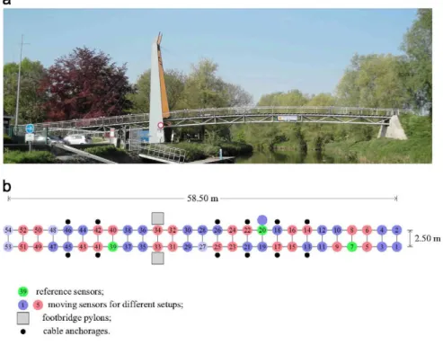
The objective of this section is to apply the proposed method to a real structure using the scheme of permanent-moving sensors. The chosen structure is a footbridge over the Dender river, in Ninove (Belgium). The Ninove footbridge is a cable-stable bridge with two pylons and six pairs of cables. The pylons split the footbridge into two spans of 36.00 m and 22.50 m. The bridge deck is a steel tubular truss. A picture of the footbridge has been included in Fig. 5(a).
A series of vibration tests were conducted on April 17 and 18, 2011 by researchers from the University of K.U. Leuven. The footbridge's dynamic response was measured with seven stations equipped with triaxial accelerometers synchronized by GPS. The measurements were carried out in a total of 13 different setups that are shown in Fig. 5(b): three stations served as references (permanently located at pools 7, 20 and 39), and the other four were used as mobile. For example, according to
Table 2
Natural frequencies and damping ratios of the modes estimated by the proposed method with permanent sensors and with overlapped sensors. MAC values are computed between estimated values and theoretical values.
Frequencies (Hz) Damping ratios
(%)
MACa
-58.501
1
' Ü
T' I I I I I
53 - 51 - 4 9 - ^ - ^ - 4 3 - 4 1 - 3 9 ^ 135 - 33 - 31 —»—
2.501
^ reference sensors;
0 £ moving sensors for different setups; footbridge pylons;
• cable anchorages.
Fig. 5. (a) Footbridge, (b) Footbridge geometry and setups location.
the figure, the first setup was composed of the pools 7, 20, 39,1, 2, 3, 4; the second one was 7, 20, 39, 5, 6, 8, 9, and so on. For each setup, time series of 10 min were collected with a sampling frequency of 200 Hz. Since the modes of interest are in the range 0-15 Hz, the data were re-sampled so that the new sampling frequency was 40 Hz (we used the Matlab function decimate).
All the measured channels are taken into account in the analysis, that is, vertical, longitudinal and transversal accelerations. This is important because in structures like this one, the mode shapes involve components in various directions.
5.2. Proposed method
All parametric system identification methods based on the state space model require to know the model order ns, which
in theory, is twice the number of identified modes. In modal testing applications it is customary to estimate the state space model for a wide range of orders and the eigenfrequencies obtained for all these orders are plotted in an eigenfrequency vs.
model order diagram, called a stabilization diagram [26]. Experience on a very large range of problems shows that in such
analysis, the eigenfrequencies corresponding to physical modes appear at most of the used model orders, while mathematical and spurious poles tend to scatter around the frequency range. Then, from such diagram it is possible to select the optimal system order, and for this order, the valid system poles.
The proposed method has been used to compute the stabilization diagram that has been plotted in Fig. 6. The
stabilization diagram can be built in the usual way because the proposed method estimates a single A and C matrices. The global mode shapes are now used to decide if the mode is stable or not.
Taking into account the stabilization diagram, we have chosen the modes estimated with a state space order equal to
ns=58. This means that 29 modes should be estimated, that is, the A matrix should have 29 pairs of complex conjugate
eigenvalues.
The results are included in Table 3. Not all the modes estimated correspond to physical modes: for example, modes 1 and 30 come from real eigenvalues; modes 7,14 and 20 have a damping ratio too high to be a structural mode. In fact, these modes are non-stable in the stabilization diagram. Other modes have low damping ratio but are non-stable:
• Modes 27, 28, 29 may be affected by the filter applied in the process to reduce the sampling frequency from 200 Hz to 40 Hz. According to the Matlab help (decimate function), the filter applied is a Chebyshev Type I filter with a cut-off frequency of 0.8 • F, where F is the new Nyquist frequency (F= 20 Hz). This means that modes with frequency higher than 16 Hz might be affected by the filter.
O 2 4 6 8 10 12 14 16 18 20 Frequency (Hz)
Fig. 6. Stabilization diagram for the Ninove footbridge with permanent sensors computed by the proposed method. The criteria are: 2% for frequencies, 5%
for damping ratios, 5% for mode shape vectors (MACs). ©: stable mode, +: unstable mode.
Table 3
Natural frequencies and damping ratios of the modes estimated by the proposed method at ns — 58.
No /(Hz) :(%) Stab. diag. Comments
9 10 11 12 13 14 15 16 17 18 19 20 21 22 23 24 25 26 27 28 29 30 1.79 2.96 2.97 3.02 3.07 3.80 4.15 5.78 6.01 6.95 8.00 8.11 8.28 8.84 9.64 9.97 10.85 11.86 12.78 12.93 13.39 13.65 14.09 14.09 14.18 14.71 16.47 17.05 17.29 19.75 1.82 0.37 5.81 1.02 1.51 33.72 2.52 0.53 0.50 1.23 5.01 1.08 31.48 12.75 1.98 1.39 2.65 2.78 47.66 2.19 0.84 1.04 6.60 6.60 0.40 4.23 1.26 0.13 Real eigenvalue Vertical bending
Lateral bending long span coupled with little torsion Lateral bending coupled with torsion
Vertical bending short span Vertical bending
Torsion long span Longitudinal mode
Torsion long span, cables zone
Torsion both spans Torsion short span Longitudinal mode Torsion
Vertical bending long span
Vertical bending short span Filter
Filter Filter Real eigenvalue
The rest of the estimated modes (i.e., modes 3, 5, 6, 8, 9,10,11 12,13,16,17,18,19, 22, 23 and 26) seem to be physical modes: they appear as stable in the stabilization diagram, the damping ratios are about 1-3%, and the mode shapes are feasible. These modes include vertical bending modes, lateral bending modes, longitudinal modes and also modes with
coupled torsion. Fig. 7 shows these identified modes. We have also drawn the position of the pylons and the cable
Mode 3. f = 2.97 Hz. ? = 0.37%
Mode 5. f = 3.07 Hz. C, = 1.02%
Mode 9. f = 6.01 Hz. C, = 0.53% Mode 10. f = 6.95 Hz. t, = 0.50%
Mode 13. f = 8.28 Hz. £ = 1.08% Mode 16. f = 9.97 Hz. X, = 1.98%
Mode 17. f = 10.85 Hz. % = 1.39% Mode 18. f = 11.86 Hz. X, = 2.65%
Mode 19. f = 12.78 Hz. X, = 2.78% Mode 22. f = 13.65 Hz. X, = 0.84%
Mode 23. f = 14.09 Hz. X, = 1.04% Mode 26. f = 14.71 Hz. £ = 0.40%
5.3. Multi-step approach using real measured data (Ninove footbridge)
Similar to the simulated case, we want to compare the results of the proposed method with the results obtained in a multi-step approach but using real measured data. We want to remark that the objective of this section is not to propose a procedure for the multi-step approach. On the contrary, we use the simplest and naive procedure (improved methods can be found in [2,7,13]). The purposes of this section are:
• To show that the process of gluing modes from individual estimates is difficult and time consuming, especially with real measured data. The procedure also requires user interaction and user expertise to merge the correct modes.
• To show the advantages of using a one-step approach, like the proposed method.
• Finally, to verify that the modes obtained with the proposed method are also obtained using the multi-step approach, that gives us confidence on the method applied to experimental data.
The SSI algorithm have been applied to the thirteen setups. We have used ns = 58, the order chosen in Table 3 and Fig. 7.
The estimated eigen-frequencies are given in Table 4. In the case of simulated data, each mode was clearly recognizable
in each setup because the natural frequencies were chosen sufficiently spaced. In contrast, the natural frequencies obtained in real structures are difficult to organize: for example, in the range (3-4 Hz) there are five values in setup 1, two values in setup 2, six in setup 3, four in setup 4, and so on; and there are very close frequencies: the mode with 3.03 Hz in setup 1 probably corresponds to the mode with 3.04 Hz in setup 2, but in setup 3 we find to modes with 3.03 Hz and 3.05 Hz. In conclusion, the problem of matching modes among setups to obtain global mode shapes is difficult, especially in structures with a high number of setups.
We have obtained some merged modes from Table 4 comparing natural frequencies, damping ratios and mode shapes
among setups. We assumed that mode i identified in setup p and mode j from setup q correspond to the same physical mode if they verified
l°}pi~°}qil<0A0, |?Pi-?q,-|<0.10, l-MAC^,}^) <Q.8Q. (42)
Table 4
Natural frequencies estimated at ns =58 by the SSI (real eigenvalues have not been removed); n^, k — 1,..., 10 stands for glued or merged mode number k taking into account Eq. (42).
Setup number
1 2 3 4 5 6 7 8 9 10 11 12 13
1.05 1.13 1.00 1.07 1.29 0.63 1.04 1.02 1.03 1.02 1.02 1.09 1.01
2.98( 1 ) 2.90 2.98( 1 ) 2.75 2.74 2.91 2.89 2.97( 1 ) 2.97( 1 ) 2.95 2.98( 1 ) 2.96( 1 ) 2.97( 1 )
3.03(2, 2.98( 1 ) 3.03 2.89 2.83 2.93 2.97( 1, 3.09(2) 3.02 2.97(i, 3.12(2, 3.07(2, 3.12(2, 3.09 3.04(2, 3.05(2) 2.93 2 . 9 8( 1, 2 . 9 8( 1, 3.06(2) 3.50 3.03 3.10(2, 3.74 3.42 3.13 3.38 3.76(3, 3.12 3.00( 1, 3.06(2, 3.03 3.35 3.85(3) 3.10(2, 3.84(3, 3.84(3, 3.82(3, 3.95(3,
3.58 4.04 3.27 3.07(2, 3.42 3.06(2, 3.35 3.93 3.16 5.76 5.85 5.77 5.25
3.76(3, 5.99 3.55 3.55 3.80(3, 3.29 3.83(3, 4.90 3.83(3, 6.01(4, 5.95 6.02(4, 6.01(4, 4.16 6.08(4, 3.77(3, 3.77(3, 4.25 3.82(3, 4.05 5.31 5.95 6.12 6.00(4, 6.97(5) 6.90
5.96 6.95(5, 4.23 4.18 5.97 4.53 4.25 5.69 6.00(4, 6.63 6.95(5, 7.92(6, 6.91(5,
6.01(4 ) 8.04(6, 5.59 6.02(4, 6.03(4, 6.02(4, 4.34 5.86 6.92(5, 6.93(5, 7.81 8.11 7.27 6.95(5, 8.51 5.73 6.89 6.94(5, 6.93(5) 6.01(4, 6.02(4) 7.31 7.85 7.97(6, 8.35 7.97(6,
7.48 9.80 6.01(4, 7.01(5, 7.47 7.31 6.26 6.95(5, 7.98(6, 7.92(6, 8.35 8.36 8.34
7.71 10.23 6.79 7.13 7.63 7.39 6.91(5, 7.96(6, 8.08 7.96 8.45 8.90 8.42
8.01(6 ) 13.05 6.93(5, 7.82 7.68 8.00(6) 8.00(6, 8.20 8.34 8.39 8.85 10.10 8.90
8.33 13.76 7.65 7.90 8.02(6, 8.10 8.19 8.23 9.23 9.36 9.85 10.28 9.00
11.05 13.99 7.98 8.02(6, 8.21 8.21 8.22 8.33 9.94 9.92 9.99 10.45 9.39
11.66 14.12(s, 8.02 8.29 8.79 8.75 8.63 9.89 10.62 10.12 10.40 10.60 10.03
12.22 14.54 8.19 10.00 9.66 9.04 9.80 10.39 10.65 10.24 10.70 10.84 10.66
12.67 14.77 9.43 10.35 11.23 9.23 9.98 11.06 11.90 10.59 11.02 11.77 11.01
14.15 15.22 9.49 10.57 11.38 11.25 10.14 11.94 11.98 10.69 12.09 12.53 12.14
14.48 15.77 9.98 11.29 11.90 11.70 12.46 12.08 12.28 11.90 12.80 13.29 12.73
14.62(9, 16.79 10.44 13.21 13.21 11.79 12.68 12.65 13.43 12.89 13.23 13.66 13.18
14.86 17.05 11.02 13.46 13.23 13.27 13.11 12.83 13.56 13.37 13.69(7, 13.88 13.42
15.06 17.13 13.26 13.47 13.38 13.63(7) 13.56(7) 13.37 13.59 13.76(7, 13.78 14.14(7, 13.69(7) 15.36 17.24( 1 0, 13.57(7, 13.62(7, 13.55(7) 13.73 14.00(3) 13.61(7) 13.67(7) 13.94 14.26(3, 14.17 13.79 16.83 17.29 13.82(8, 13.77 13.73 13.98(3, 14.71(9, 13.68 14.18(3, 14.28 14.67(9, 14.51 13.99(3) 17.27 17.31 14.72(9, 13.89(3, 13.96(3) 14.71(9, 16.62 14.02(3) 14.56 14.68(9) 15.09 14.69(9) 14.00 17.38 17.72 17.05( 1 0, 14.70(9) 14.71(9) 16.66 16.73 14.76(9) 14.67(9, 15.17 17.10 16.77 14.69(9) 17.42 18.18 17.28 16.75 16.24 16.71 17.08(10, 15.63 16.96 16.94 17.27(,o, 16.97 17.11 17.79 - 19.70 17-15(io) 16.88(,o, 17.06(,o, - 16.74 17.04(,o, 17.06 21.22 - 17.28(io)
-Table 5
Mean natural frequencies and mean damping ratios of the merged modes estimated at ns — 58 using SSI (Ninove footbridge). The corresponding modes
estimated using the proposed method are also included. The last column shows the MAC values between them (MAC is computed taking into account the global modes).
SSI Proposed method MAC Mode / ( H z )
cm
Mode /(Hz) C(%)(1) (2) (3) (4) (5) (6)
2.97 0.59 3 3.08 0.76 5 3.82 1.19 6 6.02 0.47 9 6.94 0.44 10 7.99 0.59 11
2.97 0.37 0.9192 3.07 1.02 0.6594 3.80 1.51 0.9311 6.01 0.53 0.9923 6.95 0.50 0.9906 8.00 1.23 0.8614
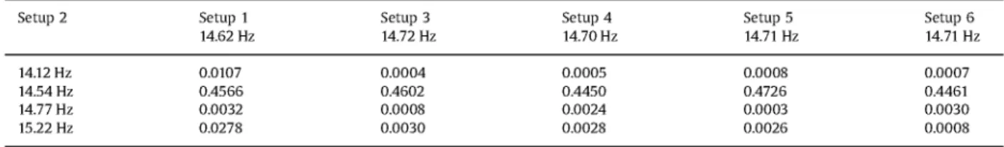
Table 6
MAC values computed between some modes estimated at setup 2 and mode (9) estimated at setups 1, 3, 4, 5 and 6 (see Table 4).
Setup 2 Setup 1 14.62 Hz Setup 3 14.72 Hz Setup 4 14.70 Hz Setup 5 14.71 Hz Setup 6 14.71 Hz 1.12 Hz 0.0107
1.54 Hz 0.4566 1.77 Hz 0.0032 .22 Hz 0.0278
0.0004 0.4602 0.0008 0.0030 0.0005 0.4450 0.0024 0.0028 0.0008 0.4726 0.0003 0.0026 0.0007 0.4461 0.0030 0.0008
where OJ¡, Q and <p¡ are defined by Eqs. (8), (9), and (10) respectively. Note that the MAC has to be computed using the
components of the modal vector <¡>¡ corresponding to the reference sensors, called here <j>¡.
These limit values are not too demanding, and of course other values can be tried. However, we only want to show some results, and to analyze the better limit values or the better procedure for the multi-step approach is out of the scope of this work. We have found six modes that verified the above conditions in the thirteen setups. The eigenfrequencies of these modes are highlighted in Table 4 with the subscripts (1), (2), (3), (4), (5) and (6). We have computed the mean eigenfrequencies and the mean damping ratios for these modes, obtaining for the eigenfrequencies: (1) 2.97 Hz, (2) 3.08 Hz, (3) 3.82 Hz, (4) 6.02 Hz, (5) 6.94 Hz, (6) 7.99 Hz. Checking the modes obtained with the proposed method, Table 3, we find values very close to them: mode 3: 2.97 Hz, mode 5: 3.07 Hz, mode 6: 3.80 Hz, mode 9: 6.01 Hz, mode 10: 6.95 Hz, mode 11: 8.00 Hz. If we compute the MAC values using the mode shapes obtained with both approaches, the results are very good, with the
exception of mode around 3.08 Hz (MAC=0.66). All these results are summarized in Table 5.
Apart from these modes, present in all the setups, we have indicated in Table 4 other modes that appear in almost all the setups: mode (9) which come up in twelve setups, mode (7) in eleven setups, and modes (8) and (10) in ten setups. They correspond for sure to vibrational modes, but the values estimated by SSI do not allow to obtain the global mode shapes. For example, let us analyze mode (9), with frequency around 14.70 Hz. It is present in all the setups except in setup 2. In this setup, there are four possible candidates: the modes with 14.12 Hz, 14.54 Hz, 14.77 Hz and 15.22 Hz. The MAC
obtained between these candidates and mode (9) estimated in other setups are given in Table 6. We see that mode with
14.54 Hz is the best candidate for mode (9) in setup 2, but the MAC with other setups is around 0.45. The conclusion is that this mode has not been properly estimated in setup 2. Maybe this mode can be improved choosing a higher order for the state space model, but this implies more modes to analyze.
On the contrary, the proposed method obtains directly the global mode shapes, their natural frequency and their damping ratios. If a mode is worse estimated in certain setups, the method uses the information of the remaining setups to obtain the global mode shape.
Table 5 shows that the multi-step mode shapes have a high MAC with the mode shapes obtained using the proposed one-step method. Besides, the mean natural frequencies computed from the multi-step are very similar to the one-step natural frequencies. And, to a lesser extent, this also happens with the damping ratios. Other modes where the multi-step approach fails, like mode (9), are estimated by the proposed method (mode 26,14.71 Hz, 0.40%). Finally, in addition to the
six complete modes and the four incomplete modes selected from Table 4, the one-step method proposes some other with
nice modal parameters (see Fig. 7).
6. Numerical example 3: gym building
-5 0 5 10 15 20 25 30 35 40 45
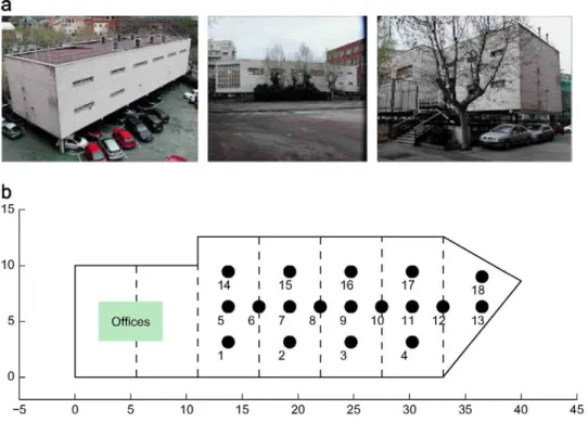
Fig. 8. (a) Gym building pictures, (b) Gym building geometry and sensor location (•); the dashed lines stand for the beams.
two stories; the second one is the gym room with 12 m wide, 22 m long (29 m if we take into account the angled end) and 6 m high. With respect to the structure, the beams and columns are made of steel, and the floors and walls are made of concrete. On September 29, 2010, the building was subjected to dynamic tests to investigate the modal parameters. The tests were conducted by researchers from the Universidad Politécnica Madrid. In total, five different setups were recorded, all vertical accelerations, with a duration of 300 s each one. Apart from the accelerometers, a 186 N shaker acting in the vertical direction was used to increase the excitation level of the structure using a chirp signal as input. The shaker position changed from one setup to the next to properly excite the structure. The accelerometers, as well as the shaker, were placed in the gym-room part.
On April 20, 2012, new setups were planned in order to measure additional points (also in the gym room). The shaker was used again to increase the excitation level. Nine setups were recorded, eight of which had the sensors at the same place while the shaker was changing position. The proposed model is able to manage these situations, and all the measurements are considered to estimate the parameters.
Table 7 summarizes the setups, the points measured at each setup and the shaker position. It is important to take into account the following remarks:
• The objective of this example is to show how the proposed model can be used to estimate the global mode shapes of a structure without using permanent sensors, that is, sensors common to all the setups. The example also shows that a sensor position can be measured more than one time, and all the measurements are used to compute the estimate. • The setups showed here are not probably the optimum: some points are measured very few and others are measured in
all the setups; or even other points should be measured in order to obtain more complete mode shapes. The optimal sensor configurations for a given structure is out of the scope of this work.
• The input signals are available, but we did not use them in our analysis. We considered the shaker input as part of the ambient excitation. We think that the results obtained under this hypothesis are valid for the purposes of this work. Nevertheless, the proposed model can be extended to take into account input signals as well. We are working on this subject and will be showed in another work.
• Mixing data measured in 2010 with data measured in 2012 has to be done with care: changes in the structure, in the environment or in the climate conditions can affect the modal parameters. As a result, the estimated modal parameters should not be used for design, structural health monitoring or other similar purposes (we only use them to show the efficiency of the method).
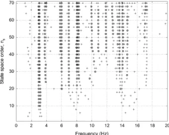
The proposed method was applied to the data and the resulting stabilization diagram is shown in Fig. 9. We have chosen
188
Table 7
Points measured in each configuration of the gym building. • means a sensor and "s" means the shaker. Measured
Point
Setups
2010 tests 2012 tests
9
10 11 12 13 14 15 16 17 18
Fig. 9. Stabilization diagram corresponding to the gym. The criteria are: 2% for frequencies, 5% for damping ratios, 5% for mode shape vectors (MAC). ©:
stable mode, + : unstable mode.
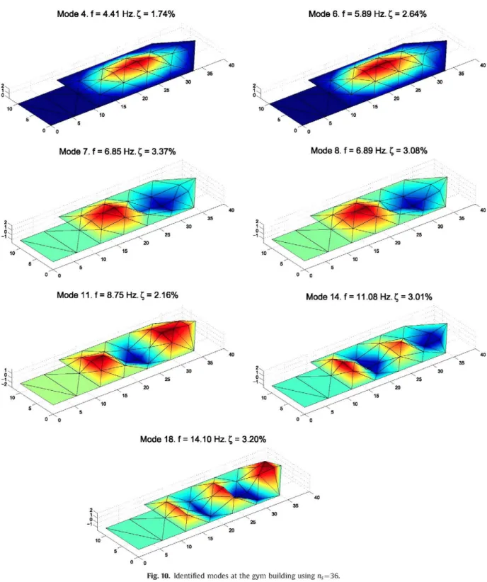
The identified mode shapes are included in Fig. 10. Modes 4 and 6 on the one hand, and modes 7 and 8 on the other hand
have very similar mode shapes at the gym room. Sensors in the offices or in horizontal directions are needed to be able to differentiate these mode shapes.
Because we used only vertical accelerometers and above all, the main excitation source was the shaker (that was vertical too), the identified modes are vertical bending ones: modes 4-6 represent the first vertical bending of the gym room; modes 7-8 the second vertical bending; mode 11 the third vertical bending; mode 14 the fourth vertical bending and finally, mode 18 the fifth vertical bending.
7. Conclusions
Estimating the modal parameters of a structure from ambient vibration measurements has become a standard methodology. In the time domain, the procedure involves the estimation of the well known state space model, for which many algorithms have been proposed. However, the model and the algorithms were developed to process one setup of sensors. When there are several setups, as in the case of estimating the mode shapes by parts, the existing methods have been adapted to try to solve the problem.
I
Mode 4. f = 4.41 Hz. ? = 1.74% Mode 6. f = 5.89 Hz. C, = 2.64%
Mode 7. f = 6.85 Hz. £ = 3.37% Mode 8. f = 6.89 Hz. £ = 3.08%
Mode 11. f = 8.75 Hz.? = 2.16% Mode 14. f = 11.08 Hz.£ = 3.01%
Mode 18. f = 14.10 Hz. £ = 3.20%
0 0
Fig. 10. Identified modes at the gym building using ns—36.
A and C matrices for all the setups that result in a single value for the natural frequency, damping ratio and global mode shape for each mode.
The stabilization diagram is made as in the case of single setups, but now the MAC values are computed using the global mode shapes. The stabilization diagram is useful to distinguish between structural modes and spurious modes.
So the problem of multiple setups of sensors can be addressed in the same way as with the well known single setup: the corresponding state space model, the algorithm to estimate the model, and the computation of the modal parameters from the model.
The proposed method has additional properties:
• The method does not need permanent sensors, but overlapped sensors can be used in place. In other words, the sensors shared by setups 1 and 2 can be different to the sensors shared by setups 1 and 3, and different to the sensors shared by setups 2 and 3, and so on. Besides, the number of overlapped can be different from one setup to the next.
• The method uses all the available data to estimate the modal parameters. Therefore, if one DOF has been measured in two different setups, the data from the two setups will be used to estimate the mode shape at this DOF. This means the estimate of the mode shapes will be better at the DOFs measured in more setups.
These properties might be used to plan more efficient tests: using a lower number of setups, measuring some places more than one time in different setups to improve the estimates, etc. These features are important in practice, and we expect them to be confirmed in further research.
Acknowledgments
This research was supported by the Ministerio de Educación y Ciencia of Spain under the research project Experimental and Computational Techniques for Dynamic Floors and Footbridges Serviceability Assessment (BIA 2011-28493-C02-01). The financial support is gratefully acknowledged.
The authors also wish to thank Prof. Guido de Roeck from KU Leuven for facilitating the access to the tests and to the experimental data of Ninove footbridge.
Appendix A. Matrix derivatives
We have used the following relationships:
J^K) =
A
(>U)
^-tr(AXB)=ATBT (A.2)
dX
^tr(AXTB) =BA (A3)
J.£r (AXBXTC) = ATCTXBT + CAXB (A. 4)
where A, B, C, X are matrices. These and other matrix formulas can be found in [24],
References
E. Reynders, System identification methods for (operational) modal analysis: review and comparison, Archives of Computational Methods in Engineering 19 (51:124) (2012).
E. Reynders, F. Magalhaes, G. De Roeck, A. Cunha, Merging strategies for multi-setup operational modal analysis: application to the Luiz I steel arch bridge, in: Proceedings of the IMAC 27, the International Modal Analysis Conference, Orlando, FL, 2009.
B. Peeters, G. De Roeck, Stochastic system identification for operational modal analysis: a review, Journal of Dynamic Systems, Measurement, and Control 123 (2001) 659-667.
H. Van der Auweraer, W. Leurs, P. Mas, L Hermans, Modal parameter estimation from inconsistent data sets, in: Proceedings of the 18th Internationa] Modal Analysis Conference (IMAC18), San Antonio, TX, 2000, pp. 763-771.
B. Cauberghe, P. Guillaume, B. Dierckx, Identification of modal parameters from inconsistent data, in: Proceedings of the 20th International Modal Analysis Conference (IMAC20), Los Angeles, CA, 2002.
R.L. Mayes, S.E. Klenke, Consolidation of modal parameters from several extraction sets, in: Proceedings of the 19th International Modal Analysis Conference (IMAC19), Orlando, FL, 2001, pp. 1023-1028.
Siu-Kui Au, Assembling mode shapes by least squares, Mechanical Systems and Signal Processing 25 (1) (January 2011) 163-179.
E. Parloo, P. Guillaume, B. Cauberghe, Maximum likelihood identification of non-stationary operational data, Journal of Sound and Vibration 268 (5) (11 December 2003) 971-991.
L Mevel, M. Basseville, A. Benveniste, M. Goursat, Merging sensor data from multiple measurement set-ups for nos-stationary subspace-based modal analysis, Journal of Sound and Vibration 249 (4) (2002) 719-741.
M. Dohler, P. Andersen, L Mevel, Data merging for multi-setup operational modal analysis with data-driven SSI, in: Proceedings of the IMAC 28, the International Modal Analysis Conference, Jacksonville, FL, 2010.
M. Dohler, E. Reynders, F. Magalhaes, L. Mevel, G. De Roeck, A. Cunha, Pre and post-identification merging for multiple-setup OMA with covariance-driven SSI, in: Proceedings of the IMAC 28, the International Modal Analysis Conference, Jacksonville, FL, 2010.
F. Magalhaes, E. Caetano, A. Cunha, O. Flamand, G. Grillaud, Ambient and free vibration tests of the Millau Viaduct: evaluation of alternative processing strategies, Engineering Structures 45 (December) (2012) 372-384.
A.P. Dempster, N.M. Laird, D.B. Rubin, Maximum likelihood from incomplete data via the EM algorithm, Journal of the Royal Statistical Society. Series B (Methodological) 39 (1) (1977) 1-38.
R.J.A. Little, D.B. Rubin, Statistical Analysis with Missing Data, 2nd ed. Wiley, New York, 2002. G.J. McLachlan, T. Krishnam, The EM algorithm and extensions, 2nd ed. Wiley, New York, 2008.
R.H. Shumway, D.S. Stoffer, An approach to time series smoothing and forecasting using the EM algorithm, Journal of Time Series Analysis 3 (4) (1982). Mark W Watson, Robert F. Engle, Alternative algorithms for the estimation of dynamic factor, mimic and varying coefficient regression models, Journal of Econometrics 23 (December (3)) (1983) 385-4000.
S.J. Koopman, Disturbance smoother for state space models, Biometrika 80 (1) (1993) 117-126.
Thomas B. Schon, Adrian Wills, Brett Ninness, System identification of nonlinear state-space models, Automática 47 (1) (2011) 39-49.
V. Digalakis, J.R. Rohlicek, M. Ostendorf, ML estimation of a stochastic linear system with the EM algorithm and its application to speech recognition, IEEE Transactions on Speech and Audio Processing 1 (October (4)) (1993) 431-442.
F.J. Cara, J. Carpió, J. Juan, E. Alaren, An approach to operational modal analysis using the expectation maximization algorithm, Mechanical Systems and Signal Processing 31 (August) (2012) 109-129.
R.H. Shumway, D.S. Stoffer, Time Series Analysis and its Aplications, 3rd ed. Springer, 2006. K.B. Petersen, M.S. Pedersen, The matrix cookbook, Version: November 14, 2008.
B. Peeters, C.E. Ventura, Comparative study of modal analysis techniques for bridge dynamic characteristics, Mechanical Systems and Signal Processing 17 (5) (2003) 965-988.