Article
Analysis of the Implementation of the Primary and
/
or
Inertial Frequency Control in Variable Speed Wind
Turbines in an Isolated Power System with High
Renewable Penetration. Case Study: El Hierro
Power System
Guillermo Martínez-Lucas1,* , JoséIgnacio Sarasúa1, Juan Ignacio Pérez-Díaz1 , Sergio Martínez2 and Danny Ochoa2
1 Department of Hydraulic, Energy and Environmental Engineering, Universidad Politécnica de Madrid,
C/Profesor Aranguren 3, 28040 Madrid, Spain; [email protected] (J.I.S.); [email protected] (J.I.P.-D.) 2 Department of Automation, Electrical Engineering and Electronics, and Industrial Informatics,
ETSI-Industriales, Universidad Politecnica de Madrid, C/Jose Gutierrez Abascal, 2, 28006 Madrid, Spain; [email protected] (S.M.); [email protected] (D.O.)
* Correspondence: [email protected]; Tel.:+34-910674333
Received: 26 April 2020; Accepted: 27 May 2020; Published: 28 May 2020
Abstract: With high levels of wind energy penetration, the frequency response of isolated power systems is more likely to be affected in the event of a sudden frequency disturbance or fluctuating wind conditions. In order to minimize excessive frequency deviations, several techniques and control strategies involving Variable Speed Wind Turbines (VSWTs) have been investigated in isolated power systems. In this paper, the main benefits and disadvantages of introducing VSWTs—both their inertial contribution and primary frequency regulation—in an exclusively renewable isolated power system have been analyzed. Special attention has been paid to the influence of the delays of control signals in the wind farm when VSWTs provide primary regulation as well as to the wind power reserve value which is needed. To achieve this objective, a methodology has been proposed and applied to a case study: El Hierro power system. A mathematical dynamic model of the isolated power system, including exclusively renewable technologies, has been described. Representative generation schedules and wind speed signals have been fixed according to the observed system. Finally, in order to obtain conclusions, realistic system events such as fluctuations in wind speed and the outage of the generation unit with the higher assigned power in the power system have been simulated.
Keywords: isolated power system; frequency regulation; variable speed wind turbine; primary frequency regulation; inertia emulation
1. Introduction
The increase in the penetration of renewable energy for electricity generation is a reality in the vast majority of countries, both in Europe and in the rest of the world. In fact, this constitutes a good way to reduce the fossil fuel dependence and greenhouse gas emissions [1]. Solar and wind-based generation systems have become sustainable and environmentally friendly options to supply power to isolated or off-grid locations, i.e., islands [2].
In recent years, the use of renewable energy sources to displace fossil fuels in small isolated systems has received considerable attention [3]. This fact has taken place largely because of the existing synergies between wind generators and Pumped Storage Hydropower Plants (PSHPs). Some remarkable works developed on the Aegean Islands analyze these synergies [4,5]. In the case
of the Faroe Islands, [6] analyzed the wind power integration combined with a variable speed PSHP. Many studies also focus on increasing the penetration of renewable energies (wind-hydro systems) in the Canary Islands [7,8]. In fact, El Hierro island aims to become 100% free from carbon dioxide emissions [9].
With high levels of wind energy penetration, especially with the large amount of Variable Speed Wind Turbines (VSWTs) incorporated into the modern utility grids, the frequency response of power systems is more likely to be affected in the event of a sudden frequency disturbance or fluctuating wind speed conditions [10]. In general, the renewable energy impact on power systems mainly depends on their penetration rate and the system inertia [11]. For this reason, the negative effects of renewable energy sources are amplified in isolated systems. In addition to its small size, the vast majority of renewable power generation technologies (except conventional hydro power plants and fixed speed wind turbines) are decoupled from the grid through a power electronic converter, implying a considerable lack of inertia in the power system [12]. For this reason, many studies analyze the impact on the frequency regulation of the penetration of renewable energies in isolated systems [13]. In order to minimize the excessive frequency deviations, several techniques and strategies involving renewable power generation technologies (mainly VSWTs) have been investigated in isolated power systems. According to [14], VSWTs can provide inertial response and primary and secondary regulation.
VSWTs’ inertial contribution consists of adding an auxiliary signal sensitive to frequency (actually, sensitive to the Rate of Change of Frequency (RoCoF)) to the reference power set point in VSWTs—for example, momentarily increasing wind turbine output power in the case of a frequency reduction. This momentary wind power increment implies a reduction in the VSWTs’ rotor speed that is corrected by the Maximum Power Point Tracking (MPPT) control [15]. Several studies are focused on the VSWTs’ conventional inertial contribution to frequency regulation [16,17]. These studies introduce the inertial action as a derivative controller monitoring the frequency error. To improve the use of variable-speed wind energy conversion systems, the conventional inertial control loop can be modified by adding a proportional loop that weights the frequency deviation, thus obtaining a Proportional–Derivative (PD) control [18]. This control loop has been later used in [19].
VSWTs’ primary frequency regulation (R1) can provide energy to assist in reducing frequency deviation, raising the frequency nadir for a given loss of supply and stabilizing the system frequency. In fact, most VSWT manufacturers now include primary frequency response capabilities as part of their offerings [20]. As for conventional power plants, the proposed control strategy requires VSWTs to preserve a power margin, so a non-optimal working point is reached in the response curve of torque versus the rotor speed of the turbine [21]. Trying to reduce this wind spill, Cortecuise et al. proposed a strategy to allow maintaining a regular reserve only when the wind turbine generator works at full load [22]. For it, a very simple system composed only of one power generator, three wind turbines and two loads was considered. The possibility to participate in R1 with a VSWT is analyzed with the help of experiments on a test bench in Reference [23]. Since only the VSWT dynamics are considered, artificial frequency variations in step form are used as the model input. Authors recognized that one of the R1 limitations was that the value of the reference power must be determined a priori. Ma and Chowdhury developed a pitch angle control—which is similar to the governor control of a synchronous machine—to provide wind plant frequency regulation capability [24]. In this case, the wind speed was assumed constant while the model input is a variation in the power demand. The assumed system consists of a synchronous generator, a VSWT and a load demand.
stresses [26]. The authors concluded that combining both inertial and primary frequency controllers improved the frequency behavior. However, they recognized as a limitation the brevity of the dynamic simulations carried out (about one minute), because they were not sufficient to characterize the reliability of the wind primary reserve. Wang and Wu proposed a distributed cooperation framework in order to improve the control efficiency for a doubly fed induction generator-based wind farm to participate in primary frequency regulation jointly with several thermal plants, including inertia emulation and droop characteristics similar to conventional plants [27].
Many times, authors do not pay special attention to the implementation of the different VSWTs control loops in the wind farms. To the authors’ knowledge, only Feltes et al. take into account the existence of communication delay between the frequency measurement and the primary control action [20]. Nevertheless, in the mentioned study, the influence of the control action delay on the dynamic response is not analyzed.
The main objective of this paper is to present a methodology to analyze the main benefits and disadvantages of introducing different control strategies in the VSWTs in an exclusively renewable isolated power system, taking into account the influence of the delays of control signals in the wind farm and the primary reserve. The proposed analysis, based on simulation results, is delivered in terms of frequency regulation, efficiency and energy indices. The isolated power system will be equipped with VSWTs, hydroelectric units, and a pump station. Hydroelectric units and the pump station are aimed to provide both primary and secondary regulation. To achieve this objective, a mathematical model including a hydropower plant, a pump station equipped with Variable Speed Pumps (VSPs) and Fix Speed Pumps (FSPs), a wind farm, the Automatic Generation Control (AGC), the power system and the power demand sensitive to the frequency deviation has been proposed. The usefulness of the results obtained from the simulations carried out with this model lies in the credibility of the simulation scenarios. The vast majority of the studies mentioned above do not include a wide variety of scenarios that enable the testing of the VSWTs’ contribution to frequency regulation. Therefore, enough representative generation schedules according to the observed system demand and wind power generation were defined. Furthermore, realistic system events that involve frequency deviations such as fluctuation in the wind speed and the outage of the generation unit with the higher assigned power have been recommended. The proposed methodology extracted from this study is applied to the El Hierro power system. El Hierro is an island in the Canary Islands archipelago. The island aims to become entirely free from greenhouse gases emissions due to a pumped storage power plant and a wind farm committed in 2014 [9].
Therefore, the main contributions of this paper are: (i) the analysis of the main benefits and disadvantages in terms of the energy, efficiency and frequency regulation of introducing different control strategies to the VSWTs in an exclusively renewable isolated power system; (ii) the consideration in said analysis of the influence of the control signal delays in the wind farm; and (iii) the generation of representative generation schedules according to the observed system demand and wind power generation.
The paper is organized as follows: In Section 2, the dynamic model is presented. The power-frequency control is described in Section 3. In Section 4, the followed methodology for generating the simulation scenarios is defined. In Section5, some realistic events are simulated considering the proposed simulation scenarios applied to El Hierro power system. Finally, Section6 outlines the main conclusions of this study.
2. Dynamic Model
sensitive to frequency deviation. The power lines’ dynamics are ignored as their influence on the frequency system is not significant [28]. The electromagnetic transients and pump station converter dynamics are supposed to be much faster than the other components of the model, so their influence in the system’s dynamics can be also omitted [29].
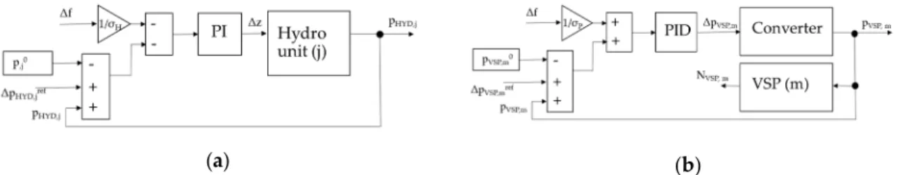
is shown in Figure 1b, is composed of a hydropower plant, a pump station equipped with VSPs and FSPs, a wind farm, the Automatic Generation Control (AGC), the power system and the power demand sensitive to frequency deviation. The power lines’ dynamics are ignored as their influence on the frequency system is not significant [28]. The electromagnetic transients and pump station converter dynamics are supposed to be much faster than the other components of the model, so their influence in the system’s dynamics can be also omitted [29].
(a) (b)
Figure 1. (a) Power system simplified one-line diagram and (b) dynamic model block diagram.
An aggregated inertial model is used for reproducing system frequency deviations because of the reduced size of the analyzed isolated power system [30]. This approximation has been successfully used by authors in the El Hierro power system [19] and by O’Sullivan et al. in the Irish one [13]. In this assumed power system, frequency deviations are the consequence of the imbalance between the power supplied by the generation units (i.e., hydroelectric units (phyd) and wind turbines
(pw)) and the power demand (i.e., VSPs (pvsp), FSPs (pfsp) and the consumers’ loads (pdem), which include
both the under frequency load-shedding scheme and their sensitivity to frequency variations through the Dnet term). Frequency variations are formulated in Equation (1).
=
, ( ) + − − − − ∆ , (1)
where Tm,hyd(t) corresponds to the mechanical starting time of the hydroelectric units and depends on
the number of units operating at each moment. Note that only the hydroelectric units provide system inertia because the FSPs, VSPs and VSWTs are connected to the grid through frequency converters.
For introducing the hydropower plant and pump station dynamic response in the model, the authors suggest models previously developed and satisfactorily used [19]. The proposed wind turbine model, which includes the wind power model and both pitch and torque MPPT control, is extracted from [31]. For the rotor mechanical model, a one-mass rotor model is used, which is enough according to [32] in cases where the power converter decouples the generator from the grid.
Finally, a load shedding scheme is added to the model as, in an isolated power system with a high penetration of renewable energies, frequency deviations may overpass thresholds associated with damage in both generating and demand equipment. This load-shedding scheme is based on the conventional Under Frequency Load Shedding (UFLS) scheme, but the RoCoF has been added as a complementary input.
3. Power-Frequency Control
The frequency control is divided into two sequential actions: primary and secondary regulation. This control scheme is assumed by many power systems in Europe. Frequency error, which is a consequence of the imbalance between power generation and power demand, is corrected initially by hydroelectric units and VSPs according to their respective droops. VSWTs are incorporated into
Figure 1.(a) Power system simplified one-line diagram and (b) dynamic model block diagram.
An aggregated inertial model is used for reproducing system frequency deviations because of the reduced size of the analyzed isolated power system [30]. This approximation has been successfully used by authors in the El Hierro power system [19] and by O’Sullivan et al. in the Irish one [13]. In this assumed power system, frequency deviations are the consequence of the imbalance between the power supplied by the generation units (i.e., hydroelectric units (phyd) and wind turbines (pw)) and the power demand (i.e., VSPs (pvsp), FSPs (pfsp) and the consumers’ loads (pdem), which include both the under frequency load-shedding scheme and their sensitivity to frequency variations through theDnetterm). Frequency variations are formulated in Equation (1).
fd f dt =
1 Tm,hyd(t)
phyd+pw−pvsp−pf sp−pd−Dnet·∆f
, (1)
whereTm,hyd(t) corresponds to the mechanical starting time of the hydroelectric units and depends on the number of units operating at each moment. Note that only the hydroelectric units provide system inertia because the FSPs, VSPs and VSWTs are connected to the grid through frequency converters.
For introducing the hydropower plant and pump station dynamic response in the model, the authors suggest models previously developed and satisfactorily used [19]. The proposed wind turbine model, which includes the wind power model and both pitch and torque MPPT control, is extracted from [31]. For the rotor mechanical model, a one-mass rotor model is used, which is enough according to [32] in cases where the power converter decouples the generator from the grid.
Finally, a load shedding scheme is added to the model as, in an isolated power system with a high penetration of renewable energies, frequency deviations may overpass thresholds associated with damage in both generating and demand equipment. This load-shedding scheme is based on the conventional Under Frequency Load Shedding (UFLS) scheme, but the RoCoF has been added as a complementary input.
3. Power-Frequency Control
Electronics2020,9, 901 5 of 24
contribution. Moreover, the inertial frequency regulation developed by VSWTs is also added in this analysis.
Permanent frequency error resulting after the action of the primary frequency control loop is rectified by secondary regulation, which is coordinated by the AGC. The AGC continuously sends increments of power reference to hydroelectric units and VSPs. The control schemes of hydroelectric units, VSPs and VSWTs are described in the following sections.
3.1. Hydroelectric Units Control Loop
The governor model of the hydroelectric units used in this study is shown in Figure2a and based on [33]. This controller monitors both the system frequency and load through the feedback signals of the frequency error and power variation. This control loop also includes the power reference provided by the AGC. The action of this governor allows eliminating the power-frequency error under electrical load variations. The error signal is processed by a conventional proportional–integral (PI) controller, producing a change in the wicket gate position. The limits in the gate position as well as its rate of change are considered in the model.
primary regulation including different control action delays in order to analyze the effect of their contribution. Moreover, the inertial frequency regulation developed by VSWTs is also added in this analysis.
Permanent frequency error resulting after the action of the primary frequency control loop is rectified by secondary regulation, which is coordinated by the AGC. The AGC continuously sends increments of power reference to hydroelectric units and VSPs. The control schemes of hydroelectric units, VSPs and VSWTs are described in the following sections.
3.1. Hydroelectric Units Control Loop
The governor model of the hydroelectric units used in this study is shown in Figure 2a and based on [33]. This controller monitors both the system frequency and load through the feedback signals of the frequency error and power variation. This control loop also includes the power reference provided by the AGC. The action of this governor allows eliminating the power-frequency error under electrical load variations. The error signal is processed by a conventional proportional–integral (PI) controller, producing a change in the wicket gate position. The limits in the gate position as well as its rate of change are considered in the model.
(a) (b)
Figure 2. Block diagram of hydro units (a) and Variable Speed Pumps (VSPs) (b) control loop.
3.2. Variable Speed Pumps Control Loop
The power consumed by the pump station can be modified to contribute to frequency regulation. As shown in Figure 2b, the VSP controller consists of a PID controller that modifies the power reference to be tracked by the converter from the frequency error and the power variation. Analogously to the hydroelectric units, this control loop includes the power reference provided by the AGC. The PI controller component proposed in [19] ensures that permanent frequency errors are corrected. The derivative component of the controller represents the synthetic inertia provided by the VSPs. Note that the pumps are connected to the system through a power converter, so inertial behavior must be emulated through the derivative component. The power converters change the electric power consumption by VSPs, reducing the frequency deviation. Therefore, the VSP rotor speed and mechanical power will adapt to the new electrical power.
3.3. Secondary Control Loop
This control action is proposed to be modelled in a similar way to [34]. Thus, the total secondary regulation effort is obtained from (2). Kf has been estimated according to the ENTSO-E recommendations. This regulation effort is distributed among all the hydroelectric units and VSPs that are synchronized as a function of their participation factors Ku,i from (3) and (4). Therefore, the sum of all the participation factors will be equal to one (5). It is assumed that all the units connected to the power system participate in secondary regulation control and the participation factors have been obtained as a function of the speed droop of each unit [35].
∆ = −∆ , (2)
∆ , =
, ∆ , , , (3)
∆ , =
, ∆ , , , (4)
Figure 2.Block diagram of hydro units (a) and Variable Speed Pumps (VSPs) (b) control loop.
3.2. Variable Speed Pumps Control Loop
The power consumed by the pump station can be modified to contribute to frequency regulation. As shown in Figure2b, the VSP controller consists of a PID controller that modifies the power reference to be tracked by the converter from the frequency error and the power variation. Analogously to the hydroelectric units, this control loop includes the power reference provided by the AGC. The PI controller component proposed in [19] ensures that permanent frequency errors are corrected. The derivative component of the controller represents the synthetic inertia provided by the VSPs. Note that the pumps are connected to the system through a power converter, so inertial behavior must be emulated through the derivative component. The power converters change the electric power consumption by VSPs, reducing the frequency deviation. Therefore, the VSP rotor speed and mechanical power will adapt to the new electrical power.
3.3. Secondary Control Loop
This control action is proposed to be modelled in a similar way to [34]. Thus, the total secondary regulation effort is obtained from (2).Kfhas been estimated according to the ENTSO-E recommendations. This regulation effort is distributed among all the hydroelectric units and VSPs that are synchronized as a function of their participation factorsKu,ifrom (3) and (4). Therefore, the sum of all the participation factors will be equal to one (5). It is assumed that all the units connected to the power system participate in secondary regulation control and the participation factors have been obtained as a function of the speed droop of each unit [35].
∆RR=−∆f·Kf, (2)
∆pHYD,jre f = 1 Tu,HYD
Z
∆RR·Ku,HYD,jdt, (3)
∆pVSP,mre f = 1 Tu,VSP
Z
X
Ku=Xj
1Ku,HYD,j+
Xm
1 Ku,VSP,m=1. (5)
3.4. Variable Speed Wind Turbines Control Loops
VSWTs can provide both inertial and primary frequency regulation. Figure3shows both the inertial and primary frequency regulation control loops of a complete wind farm. Inertial frequency regulation consists of adding an auxiliary power signal obtained from frequency variations to the reference power set point in VSWTs through a PD controller (see Equation (6)). This control action is delivered by each VSWT individually, so it is assumed that the power signal provided to the converter takes place at the same moment that the signal error is measured. The proportional component of the controller acts as a fast frequency response, monitoring the frequency deviation, while the derivative component emulates the inertial response by monitoring the RoCoF value [18,36]. For example, in response to a frequency decrease, that implies increasing the wind turbine output power momentarily from the kinetic energy stored in the rotational masses. Consequently, the rotor speed slows down (the power injected into the grid is higher than the power extracted from the wind).
∆piner=
"
Kp,iner+Kd,iner d f
dt
#
fre f−f
. (6)
Electronics 2020, 9, x FOR PEER REVIEW 7 of 24
Figure 3. Frequency control scheme of wind farm and variable speed wind turbines.
Therefore, the total power supplied by a VSWT power converter corresponds to the sum of the initial power supplied and the increments obtained from both the inertial and primary frequency regulation control loops and the VSWT speed control loop. Finally, the power supplied by the wind farm will be the sum of each VSWT’s supplied power, as in Equation (9).
= ∑ , + ∆ , + ∆ , + ∆ , . (9)
4. Methodology for Generating Simulation Scenarios
The main objective of this paper is to analyze the main benefits and disadvantages of introducing different control strategies to the VSWTs in an isolated power system, paying special attention to the influence of the delays in control signals in the wind farm. The usefulness of the results obtained from the simulations carried out with the model described in above sections lies in the credibility of the simulation scenarios. These scenarios are composed of two different parts.
The first one consists in defining enough representative generation schedules according to the observed power demand and wind power generation in the system. The second one comprises generating realistic system events that involve frequency deviations, allowing the comparison of the different control strategies. In this case, in a 100% renewable generation situation two different events have been considered: the fluctuation in the wind speed and the outage of the generation unit with the highest assigned power.
4.1. Definition of Representative 100% Renewable Generation Schedules
For the definition of representative schedules, a study of the power system demand is needed, and recorded data may be very helpful. Several demand levels can be identified and associated with a percentage of occurrence. In the same way, it is interesting to collect and analyze wind power data. These indicators can be obtained from the existing wind turbines or can be the result of future planned wind farms.
The combination of different system demands and wind power levels results in several net demands that need to be covered by a combination of hydroelectric units, VSPs and FSPs—i.e., a generation schedule. Several rules are proposed for selecting the number of components and their initial powers. Some of them are inspired in [38].
• No diesel units are scheduled.
• The same initial power is assigned to all hydroelectric units.
• The same initial power is assigned to all VSPs.
Figure 3.Frequency control scheme of wind farm and variable speed wind turbines.
The generator torque control allows variation in the VSWT rotor speed, following a MPPT strategy for extracting as much power as possible from the wind flow [37]. The reference value is the rotational speed (Equation (8)), as described in expression (7) according to [31]. This power signal is also added to be tracked by the power converter. This control loop also restores the rotational speed after the inertial controller acts, so that the power injected from the VSWT converter is smaller than the extracted wind power.
∆pω=ω
"
Kpω+Kiω
Z
dt
#
ω−ωre f. (7)
use of all the available wind energy, as this control loop introduces a power reduction if the wind power supplied grows with respect to the initial value as a consequence of an increment in the wind speed. Nevertheless, this implies that the power supplied by hydroelectric units is nearer to the initial one, therefore avoiding power deviations with respect to the programmed power.
If VSWTs contribute to primary frequency regulation, a wind power reserve is needed. In this case, the de-loading through rotational overspeed control has been used, achieving a non-optimal working point in the power–rotor speed curve of the turbine [21] as formulated in Equation (8).
ωre f =−0.75
pw
,n
1−r 2
+1.59
pw
,n
1−r
+0.63, (8)
whererrepresents the unitary proportion of the wind power reserve. For example,r=0.10 implies that the rotational speed is reduced so that the electric power supplied by VSWT,pw,n, is 10% lower than the power available from the wind.
Finally, a limitation in the rate of change of the wind farm electrical power has been introduced in the model [15]. From the point of view of VSWTs, it reduces mechanical stress [26] and, from the point of view of the system operator, sudden changes in the wind speed do not translate into strong frequency deviations.
The measurement of the controlled variables, power of each VSWT and system frequency, and estimation of the primary response signal take place in the control center of the wind farm. Because of that fact, the model includes a time delay that represents the time spent by the control action to travel from the control center to each VSWT. This delay may vary depending on the way the SCADA system interfaces with the turbine manufacturer’s park controller [20]. In this sense, the time delay depends on the type of VSWT: Type 3 (doubly fed induction machine) or Type 4 (full converter).
Therefore, the total power supplied by a VSWT power converter corresponds to the sum of the initial power supplied and the increments obtained from both the inertial and primary frequency regulation control loops and the VSWT speed control loop. Finally, the power supplied by the wind farm will be the sum of each VSWT’s supplied power, as in Equation (9).
pw=Xn i=1
pw,i0+∆piner,i+∆pω,i+∆pprim,i
. (9)
4. Methodology for Generating Simulation Scenarios
The main objective of this paper is to analyze the main benefits and disadvantages of introducing different control strategies to the VSWTs in an isolated power system, paying special attention to the influence of the delays in control signals in the wind farm. The usefulness of the results obtained from the simulations carried out with the model described in above sections lies in the credibility of the simulation scenarios. These scenarios are composed of two different parts.
The first one consists in defining enough representative generation schedules according to the observed power demand and wind power generation in the system. The second one comprises generating realistic system events that involve frequency deviations, allowing the comparison of the different control strategies. In this case, in a 100% renewable generation situation two different events have been considered: the fluctuation in the wind speed and the outage of the generation unit with the highest assigned power.
4.1. Definition of Representative 100% Renewable Generation Schedules
The combination of different system demands and wind power levels results in several net demands that need to be covered by a combination of hydroelectric units, VSPs and FSPs—i.e., a generation schedule. Several rules are proposed for selecting the number of components and their initial powers. Some of them are inspired in [38].
• No diesel units are scheduled.
• The same initial power is assigned to all hydroelectric units.
• The same initial power is assigned to all VSPs.
• The global upward reserve of the system, obtained from the sum of the reserves of each hydroelectric
unit, VSP and VSWT when they provide primary regulation, must be higher than (i) the power of the unit with the highest assigned power, the so-called N-1 criteria; or (ii) the deepest predicted ramp of wind power.
• The global downward reserve is 50% of the upward reserve.
• The wind power is limited so that the system downward reserve would not ever be overpassed. • The minimal number of pumps, compatible with the other rules, is programmed.
• VSPs are the first pumps that are scheduled.
4.2. Generation of Representative Variable Wind Speed Signals
For each of the scenarios under consideration, the response of the power system to the fluctuating speed of the wind incoming to the wind power plant is tested. Thus, the main input variable to the system is the wind speed,sw, as shown in Figure1b. As a consequence, an adequate simulation of its evolution is crucial, particularly in, but not limited to, the short term. However, wind speed fluctuations are highly dependent on atmospheric conditions and specific site characteristics, what makes their modeling difficult.
In general, wind speed can be modeled as a spatial distribution in three directions, but, assuming that the area swept by the blades of a turbine is normal to the wind direction, the model only requires a one-dimensional component. There are various alternatives for modeling the horizontal component of wind speed. Probability distributions that are useful for the estimation of energy production, like the Weibull distribution, can give approximate results. More realistic results can be obtained with Van der Hoven’s model [39] for the medium and long term, and with von Karman’s turbulence model [40] for the short term.
In the time frame of primary frequency control—the one under consideration in this work— the relevant wind speed spectrum must include both medium- and long-term fluctuations and turbulence components. Thus, a more adequate model for the wind speed numerical generator is the hybrid one proposed in [41], where the time series of wind speeds,sw(t), can be computed by addition of a medium- and long-term component,swml(t), and a turbulence component,swt(t) (Equation (10)).
sw(t) =swml(t) +swt(t). (10)
The medium- and long-term component can be calculated with a sample periodTsmlaccording to Van der Hoven’s model, as shown in Equation (11).
swml(t) =sw+XN
i=1Aicos(ωit+ϕi). (11)
This equation is limited toN=30, with uniformly distributed random phaseϕiin the interval [−π,π], and with amplitudes obtained according to the expression (12):
Ai=
p
2·[Sss(ωi) +Sss(ωi+1)]·(ωi+1−ωi)
This equation is sampled with discrete angular frequenciesωi=2π·fi/3600, wherefi is theith element of the following vector of frequencies: f = [0.001, 0.002, 0.003, 0.004, 0.005, 0.006, 0.007, 0.008, 0.009, 0.01, 0.02, 0.03, 0.04, 0.05, 0.06, 0.07, 0.08, 0.09, 0.1, 0.2, 0.3, 0.4, 0.5, 0.6, 0.7, 0.8, 0.9, 1, 2, 3] cycles/h [41], andSss(ωi) are the corresponding values of the power spectral density. These can be obtained from the power spectrum of expression (13):
Sss(ωi) =0.475σ
2L
sw
1
+ ωiL sw
!2
−5 6
, (13)
where the wind farm site is characterized by the length scale, L, and the turbulence intensity, σ, which can be estimated from [42].
For theith period of the medium- and long-term component of the wind speed,swml(t) is constant and equal toswml(i·Tsml), and the turbulent component can be calculated with a sample periodTst (a fraction ofTsml), as shown in Equation (14):
swt(t) =kσ,s·sw·nc(t), (14)
wherekσ,sis the experimental slope of the regression describing the relation between the mean value of swand the estimated value of the standard deviation.nc(t) is the output colored noise of a filter driven by white Gaussian noise with power 0 dB, according to a variant of the procedures described in [41] in which the filter transfer function for theith period is approximated by expression (15):
H(s) =KF+ (0.4TFs+1)
(TFs+1) (0.25TFs+1), (15)
whereTF=L/swml(i·Tsml) andKF=[2π/B(0.5, 1/3)TF/Tst]0.5, whereBis the beta function.
5. Case Study: El Hierro Power System
El Hierro is an island that belongs to the Canary Islands archipelago. The UNESCO declared the island as a biosphere reserve in 2000. From the energy point of view, the main task of this isolated power system is to minimize the use of fossil fuels. Traditionally, diesel groups (15 MW) covered the demand of the island (a 7.7 MW peak and a 2.1 MW valley in 2018). Thus, in 2014 Gorona del Viento Wind Pumped storage power plant was commissioned—see Figure4. The wind farm is formed of five 2.3 MW ENERCON E-70 VSWTs (type 4), and the pumped storage power plant is equipped with 4×2.8 MW Pelton turbines, 6×0.5 MW FSPs and 2×1.5 MW VSPs. The main data and characteristics
of the system that define the dynamic model are reported in [19].
Electronics 2020, 9, x FOR PEER REVIEW 9 of 24
( ) = , ( ), (14)
where kσ,s is the experimental slope of the regression describing the relation between the mean value of sw and the estimated value of the standard deviation. nc(t) is the output colored noise of a filter driven by white Gaussian noise with power 0 dB, according to a variant of the procedures described in [41] in which the filter transfer function for the ith period is approximated by expression (15):
( ) = +( ( . ) ( . ) ), (15)
where TF = L/swml(i·Tsml) and KF = [2π/B(0.5, 1/3) TF/Tst]0.5, where B is the beta function.
5. Case Study: El Hierro Power System
El Hierro is an island that belongs to the Canary Islands archipelago. The UNESCO declared the island as a biosphere reserve in 2000. From the energy point of view, the main task of this isolated power system is to minimize the use of fossil fuels. Traditionally, diesel groups (15 MW) covered the demand of the island (a 7.7 MW peak and a 2.1 MW valley in 2018). Thus, in 2014 Gorona del Viento Wind Pumped storage power plant was commissioned—see Figure 4.The wind farm is formed of five 2.3 MW ENERCON E-70 VSWTs (type 4), and the pumped storage power plant is equipped with 4 × 2.8 MW Pelton turbines, 6 × 0.5 MW FSPs and 2 × 1.5 MW VSPs. The main data and characteristics of the system that define the dynamic model are reported in [19].
Figure 4. Gorona del Viento Wind–Hydro power plant.
In the last two years, the participation of renewable energy has grown significantly. In the summer of 2019, for 596 consecutive hours the electric demand was continuously and exclusively supplied by renewable energy resources. However, this significant milestone presents an important operational disadvantage—the difficulty in controlling the power system frequency due to wind power variations. This problem is aggravated by the lack of system inertia, inherent in VSWTs connected to the system through power electronic equipment, so that load shedding is a common practice, especially when using FSPs [43]. In this context, the contribution of VSWTs to frequency regulation becomes an important means to respond to the challenge of a generation 100% free of greenhouse gas emissions. In spite of the pump station, the hydropower plant and VSWTs’ contribution to frequency regulation, frequency nadir can reach unacceptable values due to excessive power excursions. To correct these frequency deviations, a load-shedding scheme is implemented in the power system, as shown in Table 1.
Table 1. Load-shedding scheme characteristics in El Hierro isolated power system.
UFLS Stages
Frequency Threshold (Hz)
RoCoF Threshold
(mHz/s) Delay (s)
Load Shedding Percentage (%)
1 48.5 800 0.1 12.5
2 48.2 800 0.2 12.5
In the last two years, the participation of renewable energy has grown significantly. In the summer of 2019, for 596 consecutive hours the electric demand was continuously and exclusively supplied by renewable energy resources. However, this significant milestone presents an important operational disadvantage—the difficulty in controlling the power system frequency due to wind power variations. This problem is aggravated by the lack of system inertia, inherent in VSWTs connected to the system through power electronic equipment, so that load shedding is a common practice, especially when using FSPs [43]. In this context, the contribution of VSWTs to frequency regulation becomes an important means to respond to the challenge of a generation 100% free of greenhouse gas emissions. In spite of the pump station, the hydropower plant and VSWTs’ contribution to frequency regulation, frequency nadir can reach unacceptable values due to excessive power excursions. To correct these frequency deviations, a load-shedding scheme is implemented in the power system, as shown in Table1.
Table 1.Load-shedding scheme characteristics in El Hierro isolated power system.
UFLS Stages Frequency Threshold (Hz) RoCoF Threshold (mHz/s) Delay (s) Load Shedding Percentage (%)
1 48.5 800 0.1 12.5
2 48.2 800 0.2 12.5
3 47.8 800 0.4 12.5
4 47.5 800 0.6 12.5
5.1. Generation of 100% Renewable Scenarios
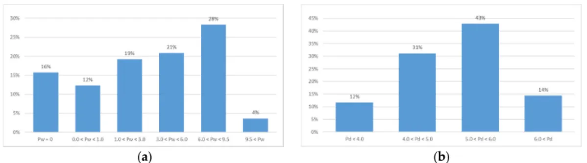
Following the methodology presented in the previous section, data from El Hierro power system have been collected, in particular wind power production and demand during 2018. Wind power data have been divided into six different intervals and system electric demand in four ranges. The distribution of these ranges during 2018 are represented in Figure5.
Electronics 2020, 9, x FOR PEER REVIEW 10 of 24
3 47.8 800 0.4 12.5
4 47.5 800 0.6 12.5
5.1. Generation of 100% Renewable Scenarios
Following the methodology presented in the previous section, data from El Hierro power system have been collected, in particular wind power production and demand during 2018. Wind power data have been divided into six different intervals and system electric demand in four ranges. The distribution of these ranges during 2018 are represented in Figure 5.
(a) (b)
Figure 5. 2018 El Hierro power system distributions of (a) wind power and (b) power demand.
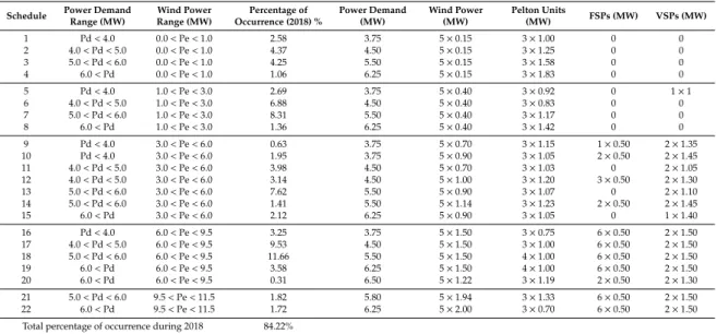
The combination of both demand and wind power ranges leads to the definition of 22 different schedules—see Table 2. Obviously, the schedules related to no wind power (16% in Figure 5a) have not been included. Some possible combinations have not been included either because they have not been registered during 2018. In Table 2, there are some schedules with the same demand and wind power range, but they correspond to different cases of power demand that are higher or lower than the wind power. The resulting net demand is covered by Pelton units and pumps following the rules listed in the section above. The pump station is particularly necessary when the wind power is higher than the demand (negative net demand). Each schedule is associated with a percentage of occurrence according to 2018 data. The sum of all the percentages is 84.22%.
Table 2. Twenty-two generated schedules and its associated percentage of occurrence during 2018.
Schedule Power Demand
Range (MW) Wind Power Range (MW) Percentage of Occurrence (2018) % Power Demand (MW) Wind Power (MW) Pelton Units (MW) FSPs (MW) VSPs (MW)
1 Pd < 4.0 0.0 < Pe < 1.0 2.58 3.75 5 × 0.15 3 × 1.00 0 0 2 4.0 < Pd < 5.0 0.0 < Pe < 1.0 4.37 4.50 5 × 0.15 3 × 1.25 0 0 3 5.0 < Pd < 6.0 0.0 < Pe < 1.0 4.25 5.50 5 × 0.15 3 × 1.58 0 0 4 6.0 < Pd 0.0 < Pe < 1.0 1.06 6.25 5 × 0.15 3 × 1.83 0 0 5 Pd < 4.0 1.0 < Pe < 3.0 2.69 3.75 5 × 0.40 3 × 0.92 0 1 × 1 6 4.0 < Pd < 5.0 1.0 < Pe < 3.0 6.88 4.50 5 × 0.40 3 × 0.83 0 0 7 5.0 < Pd < 6.0 1.0 < Pe < 3.0 8.31 5.50 5 × 0.40 3 × 1.17 0 0 8 6.0 < Pd 1.0 < Pe < 3.0 1.36 6.25 5 × 0.40 3 × 1.42 0 0 9 Pd < 4.0 3.0 < Pe < 6.0 0.63 3.75 5 × 0.70 3 × 1.15 1 × 0.50 2 × 1.35 10 Pd < 4.0 3.0 < Pe < 6.0 1.95 3.75 5 × 0.90 3 × 1.05 2 × 0.50 2 × 1.45 11 4.0 < Pd < 5.0 3.0 < Pe < 6.0 3.98 4.50 5 × 0.70 3 × 1.03 0 2 × 1.05 12 4.0 < Pd < 5.0 3.0 < Pe < 6.0 3.14 4.50 5 × 1.00 3 × 1.20 3 × 0.50 2 × 1.30 13 5.0 < Pd < 6.0 3.0 < Pe < 6.0 7.62 5.50 5 × 0.90 3 × 1.07 0 2 × 1.10 14 5.0 < Pd < 6.0 3.0 < Pe < 6.0 1.41 5.50 5 × 1.14 3 × 1.23 2 × 0.50 2 × 1.45 15 6.0 < Pd 3.0 < Pe < 6.0 2.12 6.25 5 × 0.90 3 × 1.05 0 1 × 1.40 16 Pd < 4.0 6.0 < Pe < 9.5 3.25 3.75 5 × 1.50 3 × 0.75 6 × 0.50 2 × 1.50 17 4.0 < Pd < 5.0 6.0 < Pe < 9.5 9.53 4.50 5 × 1.50 3 × 1.00 6 × 0.50 2 × 1.50 18 5.0 < Pd < 6.0 6.0 < Pe < 9.5 11.66 5.50 5 × 1.50 4 × 1.00 6 × 0.50 2 × 1.50 19 6.0 < Pd 6.0 < Pe < 9.5 3.58 6.25 5 × 1.50 4 × 1.00 6 × 0.50 2 × 1.50 20 6.0 < Pd 6.0 < Pe < 9.5 0.31 6.50 5 × 1.22 3 × 1.19 2 × 0.50 2 × 1.30
21 5.0 < Pd < 6.0 9.5 < Pe <
11.5 1.82 5.80 5 × 1.94 3 × 1.33 6 × 0.50 2 × 1.50 Figure 5.2018 El Hierro power system distributions of (a) wind power and (b) power demand.
The combination of both demand and wind power ranges leads to the definition of 22 different schedules—see Table2. Obviously, the schedules related to no wind power (16% in Figure5a) have not been included. Some possible combinations have not been included either because they have not been registered during 2018. In Table2, there are some schedules with the same demand and wind power range, but they correspond to different cases of power demand that are higher or lower than the wind power. The resulting net demand is covered by Pelton units and pumps following the rules listed in the section above. The pump station is particularly necessary when the wind power is higher than the demand (negative net demand). Each schedule is associated with a percentage of occurrence according to 2018 data. The sum of all the percentages is 84.22%.
Table 2.Twenty-two generated schedules and its associated percentage of occurrence during 2018.
Schedule Power DemandRange (MW) Range (MW)Wind Power Occurrence (2018) %Percentage of Power Demand(MW) Wind Power(MW) Pelton Units(MW) FSPs (MW) VSPs (MW)
1 Pd<4.0 0.0<Pe<1.0 2.58 3.75 5×0.15 3×1.00 0 0 2 4.0<Pd<5.0 0.0<Pe<1.0 4.37 4.50 5×0.15 3×1.25 0 0 3 5.0<Pd<6.0 0.0<Pe<1.0 4.25 5.50 5×0.15 3×1.58 0 0 4 6.0<Pd 0.0<Pe<1.0 1.06 6.25 5×0.15 3×1.83 0 0 5 Pd<4.0 1.0<Pe<3.0 2.69 3.75 5×0.40 3×0.92 0 1×1 6 4.0<Pd<5.0 1.0<Pe<3.0 6.88 4.50 5×0.40 3×0.83 0 0 7 5.0<Pd<6.0 1.0<Pe<3.0 8.31 5.50 5×0.40 3×1.17 0 0 8 6.0<Pd 1.0<Pe<3.0 1.36 6.25 5×0.40 3×1.42 0 0 9 Pd<4.0 3.0<Pe<6.0 0.63 3.75 5×0.70 3×1.15 1×0.50 2×1.35 10 Pd<4.0 3.0<Pe<6.0 1.95 3.75 5×0.90 3×1.05 2×0.50 2×1.45 11 4.0<Pd<5.0 3.0<Pe<6.0 3.98 4.50 5×0.70 3×1.03 0 2×1.05 12 4.0<Pd<5.0 3.0<Pe<6.0 3.14 4.50 5×1.00 3×1.20 3×0.50 2×1.30 13 5.0<Pd<6.0 3.0<Pe<6.0 7.62 5.50 5×0.90 3×1.07 0 2×1.10 14 5.0<Pd<6.0 3.0<Pe<6.0 1.41 5.50 5×1.14 3×1.23 2×0.50 2×1.45 15 6.0<Pd 3.0<Pe<6.0 2.12 6.25 5×0.90 3×1.05 0 1×1.40 16 Pd<4.0 6.0<Pe<9.5 3.25 3.75 5×1.50 3×0.75 6×0.50 2×1.50 17 4.0<Pd<5.0 6.0<Pe<9.5 9.53 4.50 5×1.50 3×1.00 6×0.50 2×1.50 18 5.0<Pd<6.0 6.0<Pe<9.5 11.66 5.50 5×1.50 4×1.00 6×0.50 2×1.50 19 6.0<Pd 6.0<Pe<9.5 3.58 6.25 5×1.50 4×1.00 6×0.50 2×1.50 20 6.0<Pd 6.0<Pe<9.5 0.31 6.50 5×1.22 3×1.19 2×0.50 2×1.30 21 5.0<Pd<6.0 9.5<Pe<11.5 1.82 5.80 5×1.94 3×1.33 6×0.50 2×1.50 22 6.0<Pd 9.5<Pe<11.5 1.72 6.25 5×2.00 3×0.70 6×0.50 2×1.50 Total percentage of occurrence during 2018 84.22%
Four different control strategies are implemented in VSWTs:
- No control action (base case). - Inertial response.
- Primary regulation (R1).
- Inertial response and primary regulation acting together.
The VSWTs’ regulation action, when they are asked to provide primary regulation, depends on the regulation reserve. In this paper, two different reserves are considered: 5% and 10% of the initial wind power (r=0.05 and r=0.10).
Finally, as described in Section3.4, primary regulation is coordinated by “the wind farm control”, which sends the control signal to the VSWTs. This process involves a delay that may worsen the regulation results. In [20], this delay is quantified as 500 ms for VSWTs of type 3 and 1500 ms for VSWTs of type 4. In this research work, even though the VSWTs in El Hierro are type 4, three different cases are compared: no delay, 500 ms delay and 1500 ms delay.
In next subsections, the results of varying schedule, control strategy, primary reserve and R1 time delay are presented.
5.2. Variable Wind Speed Simulations Results
According to the methodology described in previous sections, a total number of 22 schedules associated to wind speed signal have been obtained. The four analyzed VSWTs control strategies, the two different wind power reserves and the three primary regulation delays have been simulated. For that reason, in order to clarify the obtained results, both the average values of the 22 schedules and their 95% confidence intervals of different quality parameters are listed in the following tables. The 95% confidence intervals have been obtained according to expression (16), assuming that all values fit a Student’s t-Distribution, as the sample size is below thirty [44].
x±t(α,n)Sm. (16)
the VSWTs provide primary frequency regulation, reducing both frequency extreme values and MSE. Likewise, the worst value of RoCoF is further reduced because of the inertial regulation. The joint action of both inertial contribution and primary regulation improves the response of the system, but not significantly. Analogously, the increase in the primary regulation power reserve does not substantially improve the quality of the frequency either. VSWTs primary regulation reserve implies that both Pelton units and VSWTs initially supplied a different power value than if VSWTs provided inertial contribution. According to [29], the quality of the frequency would improve if the controllers’ gains of Pelton units and VSWTs changed to the proper ones associated to the real operating point. Moreover, including VSWTs primary control delay influences negatively the frequency quality parameters, highlighting the importance of its inclusion in the model.
Table 3.Average values of the twenty-two schedules of frequency parameters considering proposed VSWTs contributions, reserves and delays.
VSWT Contribution VSWT Reserve VSWT R1 Delay
Frequency Parameters
Nadir Max F MSE Min. RoCoF (Hz) (Hz) 10−5p.u. (Hz/s) None - - 48.6292±0.2116 51.3270±0.1396 11.1±2.57 −0.5603±0.1742
Inertial - - 48.8521±0.2079 51.1242±0.1417 8.40±1.90 −0.2888±0.0350
R1 5%
0
48.9382±0.1956 51.0997±0.1462 7.77±1.84 −0.3582±0.0737
R1 10% 48.9689±0.1924 51.0931±0.1390 7.67±1.77 −0.3151±0.0538
Inertial and R1 5% 49.0448±0.1895 50.9427±0.1260 6.30±1.61 −0.2426±0.0362
Inertial and R1 10% 49.0754±0.1866 50.9550±0.1312 6.12±1.52 −0.2409±0.0370
R1 5%
500 ms
48.9360±0.1951 51.1047±0.1489 7.62±1.75 −0.3472±0.0540
R1 10% 48.9626±0.1916 51.0930±0.1400 7.57±1.72 −0.3625±0.0669
Inertial and R1 5% 49.0459±0.1905 50.9495±0.1272 6.06±1.45 −0.2751±0.0632
Inertial and R1 10% 49.0758±0.1877 50.9606±0.1316 5.80±1.34 −0.2476±0.0385
R1 5%
1500 ms
48.8663±0.1872 51.1544±0.1523 8.05±1.73 −0.3933±0.0583
R1 10% 48.8880±0.1828 51.1531±0.1472 7.91±1.64 −0.4080±0.0637
Inertial and R1 5% 49.0450±0.1922 50.9704±0.1323 6.14±1.51 −0.3037±0.0709
Inertial and R1 10% 49.0726±0.1888 50.9784±0.1363 5.98±1.42 −0.2652±0.0411
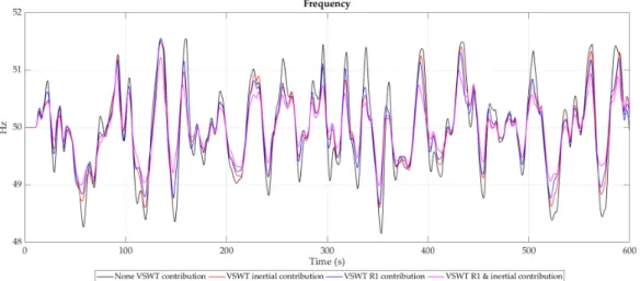
Figure6, which contains graphical results obtained from schedule number 13 taken as an example, shows the frequency dynamic response assuming the different VSWTs control strategies. As can be seen, the upper and lower values of the frequency improve, approaching the nominal frequency of the system, thanks to the contribution of the VSWTs.
Electronics 2020, 9, x FOR PEER REVIEW 12 of 24
VSWT Contribution
VSWT Reserve
VSWT R1 Delay
Frequency Parameters
Nadir Max F MSE Min. RoCoF
(Hz) (Hz) 10−5 p.u. (Hz/s)
None - - 48.6292 ± 0.2116 51.3270 ± 0.1396 11.1 ± 2.57 −0.5603 ± 0.1742 Inertial - - 48.8521 ± 0.2079 51.1242 ± 0.1417 8.40 ± 1.90 −0.2888 ± 0.0350
R1 5%
0
48.9382 ± 0.1956 51.0997 ± 0.1462 7.77 ± 1.84 −0.3582 ± 0.0737 R1 10% 48.9689 ± 0.1924 51.0931 ± 0.1390 7.67 ± 1.77 −0.3151 ± 0.0538 Inertial and R1 5% 49.0448 ± 0.1895 50.9427 ± 0.1260 6.30 ± 1.61 −0.2426 ± 0.0362 Inertial and R1 10% 49.0754 ± 0.1866 50.9550 ± 0.1312 6.12 ± 1.52 −0.2409 ± 0.0370
R1 5%
500 ms
48.9360 ± 0.1951 51.1047 ± 0.1489 7.62 ± 1.75 −0.3472 ± 0.0540 R1 10% 48.9626 ± 0.1916 51.0930 ± 0.1400 7.57 ± 1.72 −0.3625 ± 0.0669 Inertial and R1 5% 49.0459 ± 0.1905 50.9495 ± 0.1272 6.06 ± 1.45 −0.2751 ± 0.0632 Inertial and R1 10% 49.0758 ± 0.1877 50.9606 ± 0.1316 5.80 ± 1.34 −0.2476 ± 0.0385
R1 5%
1500 ms
48.8663 ± 0.1872 51.1544 ± 0.1523 8.05 ± 1.73 −0.3933 ± 0.0583 R1 10% 48.8880 ± 0.1828 51.1531 ± 0.1472 7.91 ± 1.64 −0.4080 ± 0.0637 Inertial and R1 5% 49.0450 ± 0.1922 50.9704 ± 0.1323 6.14 ± 1.51 −0.3037 ± 0.0709 Inertial and R1 10% 49.0726 ± 0.1888 50.9784 ± 0.1363 5.98 ± 1.42 −0.2652 ± 0.0411
Figure 6, which contains graphical results obtained from schedule number 13 taken as an example, shows the frequency dynamic response assuming the different VSWTs control strategies. As can be seen, the upper and lower values of the frequency improve, approaching the nominal frequency of the system, thanks to the contribution of the VSWTs.
Figure 6. Frequency dynamic response in the cases none VSWT contribution, VSWT inertial contribution, primary frequency regulation (R1) contribution and R1 and inertial contribution (5% power reserve).
Table 4 lists the average values of the hydraulic parameters: pumped and turbined water volumes and the sum of the wicket gate movements. On the one hand, pumped values do not vary significantly, regardless of the type of VSWT control strategy. Note that, according to the criteria described in Section 4.1, the initial power consumed by the pumps has remained constant in each scenario, regardless of the type of contribution of the VSWTs. Therefore, small variations depend on the control effort of the VSPs. However, it is appreciated that the inertial contribution of the VSWTs allows a small saving in pumped volume, acting both individually and together with the primary regulation.
On the other hand, the turbined volume is affected by the VSWT regulation strategy. As previously indicated, the VSWTs’ primary regulation requires maintaining a power regulation reserve, reducing the power they supply. For this reason, Pelton units must compensate for this reduction, increasing their power and, therefore, the turbined water volume. The greater the R1 regulation reserve, the greater the increase in turbined water volume. Adding inertial response or considering control delay does not affect the water volumes.
Figure 6.Frequency dynamic response in the cases none VSWT contribution, VSWT inertial contribution, primary frequency regulation (R1) contribution and R1 and inertial contribution (5% power reserve).
regardless of the type of VSWT control strategy. Note that, according to the criteria described in Section4.1, the initial power consumed by the pumps has remained constant in each scenario, regardless of the type of contribution of the VSWTs. Therefore, small variations depend on the control effort of the VSPs. However, it is appreciated that the inertial contribution of the VSWTs allows a small saving in pumped volume, acting both individually and together with the primary regulation.
Table 4.Average values of hydraulic parameters considering the proposed VSWT contributions.
VSWT Contribution VSWT Reserve VSWT R1 Delay Pumped Volume Turbined Volume
R (∆z)dt
t
(m3) (m3) 10−4(p.u.)
None - - 276.70±103.01 211.29±17.66 4.16±0.554
Inertial - - 275.42±103.36 210.63±17.76 2.42±0.158
R1 5%
0
275.88±103.55 216.16±17.68 4.08±0.525
R1 10% 276.38±103.76 222.01±17.99 3.88±0.302
Inertial and R1 5% 275.25±103.79 216.98±17.88 1.73±0.081
Inertial and R1 10% 275.91±104.05 222.73±18.25 1.80±0.085
R1 5%
500 ms
275.97±103.57 216.25±17.68 3.89±0.029
R1 10% 276.50±103.79 222.09±17.99 3.85±0.399
Inertial and R1 5% 275.35±103.82 216.98±17.88 1.77±0.085
Inertial and R1 10% 276.00±104.08 222.74±18.25 1.77±0.087
R1 5%
1500 ms
276.15±103.55 216.43±17.67 2.35±0.163
R1 10% 276.78±103.77 222.22±17.98 2.40±0.206
Inertial and R1 5% 275.48±103.85 217.03±17.91 1.79±0.092
Inertial and R1 10% 276.11±104.09 222.79±18.26 1.86±0.964
On the other hand, the turbined volume is affected by the VSWT regulation strategy. As previously indicated, the VSWTs’ primary regulation requires maintaining a power regulation reserve, reducing the power they supply. For this reason, Pelton units must compensate for this reduction, increasing their power and, therefore, the turbined water volume. The greater the R1 regulation reserve, the greater the increase in turbined water volume. Adding inertial response or considering control delay does not affect the water volumes.
The main advantage of VSWTs’ contribution to frequency regulation in terms of hydraulic parameters lies in the gate opening movements of the hydroelectric units, measured through the sum of their increments. The largest increases take place when the VSWTs provide inertial and primary regulation together. This reduction is significant, even taking into account the R1 control action delay, and it implies an extension of the remaining lifetime of the turbine components.
Table5lists the average values of the VSWT parameters: the total energy supplied by the VSWTs and the sum of blade movements. As expected, there is a decrease in the energy supplied by the VSWTs when they provide R1 due to the need to maintain a regulation power reserve. A wind spill occurs because a non-optimal working point in the power–rotor speed curve of the turbine is achieved. This is also verified in Figure7, which contains graphical results obtained from schedule number 13 taken as an example. It can be seen how the higher values of wind power obtained when VSWTs do not provide R1 are not reached by the generated power in the cases in which VSWTs provide R1. However, there is also a small increase in the wind energy supplied due to the inertial regulation of the VSWTs. The supplied wind energy is not affected by the R1control action delay.
Table 5.Average values of VSWT parameters considering the proposed VSWT contributions.
VSWT Contribution VSWT Reserve VSWT R1 Delay Wind Energy
R (∆β)dt
t
(kWh) 10−2(p.u.)
None - - 626.49±171.48 3.33±0.680
Inertial - - 630.71±170.65 3.27±0.188
R1 5%
0
613.50±165.36 3.95±0.769
R1 10% 595.54±159.96 5.39±0.243
Inertial and R1 5% 612.99±164.22 2.73±0.166
Inertial and R1 10% 595.66±159.05 2.91±0.136
R1 5%
500 ms
613.13±165.39 5.51±0.288
R1 10% 595.19±159.95 5.43±0.348
Inertial and R1 5% 612.94±164.27 2.88±0.140
Inertial and R1 10% 595.57±159.09 2.91±0.173
R1 5%
1500 ms
612.18±165.46 3.35±0.224
R1 10% 594.39±159.97 3.35±0.241
Inertial and R1 5% 612.57±164.31 2.96±0.111
Inertial and R1 10% 595.13±159.04 3.12±0.112
Electronics 2020, 9, x FOR PEER REVIEW 14 of 24
R1 5% 0
613.50 ± 165.36 3.95 ± 0.769 R1 10% 595.54 ± 159.96 5.39 ± 0.243 Inertial and R1 5% 612.99 ± 164.22 2.73 ± 0.166 Inertial and R1 10% 595.66 ± 159.05 2.91 ± 0.136
R1 5% 500 ms
613.13 ± 165.39 5.51 ± 0.288 R1 10% 595.19 ± 159.95 5.43 ± 0.348 Inertial and R1 5% 612.94 ± 164.27 2.88 ± 0.140 Inertial and R1 10% 595.57 ± 159.09 2.91 ± 0.173
R1 5% 1500 ms
612.18 ± 165.46 3.35 ± 0.224 R1 10% 594.39 ± 159.97 3.35 ± 0.241 Inertial and R1 5% 612.57 ± 164.31 2.96 ± 0.111 Inertial and R1 10% 595.13 ± 159.04 3.12 ± 0.112
Figure 7. Wind power production in the cases none VSWT contribution, VSWT inertial contribution, R1 contribution and R1 and inertial contribution (5% power reserve).
Figure 8. Blade position in the cases none VSWT contribution, VSWT inertial contribution, R1 contribution and R1 and inertial contribution (5% power reserve), respectively.
Table 6 collects the influence of the VSWT regulation strategies on the annual supplied wind energy and the hydraulic balance of the hydropower plant (pumped volume of water minus turbined volume of water). These data are extended listing schedule by schedule in Table A3 in Appendix A.
Figure 7.Wind power production in the cases none VSWT contribution, VSWT inertial contribution, R1 contribution and R1 and inertial contribution (5% power reserve).
Electronics 2020, 9, x FOR PEER REVIEW 14 of 24
R1 5%
0
613.50 ± 165.36 3.95 ± 0.769
R1 10% 595.54 ± 159.96 5.39 ± 0.243
Inertial and R1 5% 612.99 ± 164.22 2.73 ± 0.166 Inertial and R1 10% 595.66 ± 159.05 2.91 ± 0.136
R1 5%
500 ms
613.13 ± 165.39 5.51 ± 0.288
R1 10% 595.19 ± 159.95 5.43 ± 0.348
Inertial and R1 5% 612.94 ± 164.27 2.88 ± 0.140 Inertial and R1 10% 595.57 ± 159.09 2.91 ± 0.173
R1 5%
1500 ms
612.18 ± 165.46 3.35 ± 0.224
R1 10% 594.39 ± 159.97 3.35 ± 0.241
Inertial and R1 5% 612.57 ± 164.31 2.96 ± 0.111 Inertial and R1 10% 595.13 ± 159.04 3.12 ± 0.112
Figure 7. Wind power production in the cases none VSWT contribution, VSWT inertial contribution, R1 contribution and R1 and inertial contribution (5% power reserve).
Figure 8. Blade position in the cases none VSWT contribution, VSWT inertial contribution, R1 contribution and R1 and inertial contribution (5% power reserve), respectively.
Table 6 collects the influence of the VSWT regulation strategies on the annual supplied wind energy and the hydraulic balance of the hydropower plant (pumped volume of water minus turbined volume of water). These data are extended listing schedule by schedule in Table A3 in Appendix A.
These wide variations obstruct the blade position adaptation to the needs of the wind turbine due to the limitation in the speed of its movements.
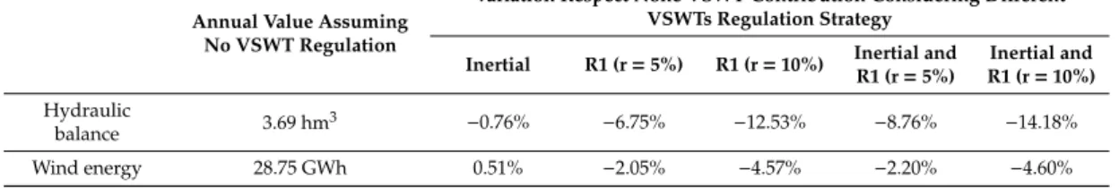
Table6collects the influence of the VSWT regulation strategies on the annual supplied wind energy and the hydraulic balance of the hydropower plant (pumped volume of water minus turbined volume of water). These data are extended listing schedule by schedule in TableA3in AppendixA. The annual values have been calculated as the weighted average with respect to the percentage of occurrence of each generation schedule for the year 2018. It is important to notice the variability of the data contained in the mentioned TableA3in contrast with the final values of Table6. Both the wind energy and hydraulic balance heavily depend on the programmed schedule. For example, in the case of only 10% R1 reserve, the wind energy is reduced from 2.13% in schedule 15 to 8.74% in schedule 22 with respect to the base case with no VSWT regulation. The same performance can be observed in the case of water balance. For the same control strategy, in schedule 5 the volume of pumped water is improved by 23%, and in schedule 13 it is reduced by 39.4%. This fact highlights the use of multiple programmed schedules proposed in the methodology of this paper in order to obtain a wide vision of the matter.
Table 6.Aggregated comparison of the hydraulic balance (difference between pumped and turbined volume) and wind energy produced between none VSWT contribution and the proposed VSWT regulation strategy.
Annual Value Assuming No VSWT Regulation
Variation Respect None VSWT Contribution Considering Different VSWTs Regulation Strategy
Inertial R1 (r=5%) R1 (r=10%) Inertial and R1 (r=5%)
Inertial and R1 (r=10%)
Hydraulic
balance 3.69 hm3 −0.76% −6.75% −12.53% −8.76% −14.18%
Wind energy 28.75 GWh 0.51% −2.05% −4.57% −2.20% −4.60%
Due to the contribution of the VSWTs to primary frequency regulation, it is verified that there is a decrease in the annual hydraulic balance—that is, a reduction in the pumped water volume and an increase in the turbined volume. On the one hand, the reduction in the pumped volume is due to the decrease in the wind energy supplied—that is, the power consumed by the pumps decreases due to a deficit in wind energy production. On the other hand, this reduction in the wind energy-supplied due to the contribution of VSWTs to frequency regulation causes the energy produced by the Pelton units to increase, implying an increase in the turbinated water volume. In the case of inertial contribution, this effect is limited.
Regarding the annual wind energy supplied by the wind farm, a clear reduction is seen when the VSWTs provide R1 due to the requirement to maintain a power reserve and be operating below their optimum production curve. This means that the improvement in the quality of the frequency takes place at the cost of a reduction in the energy efficiency of the system. Undoubtedly, this annual energy loss is greater the larger the power regulation reserve maintained. However, the proportion of wind energy reduction is much lower than the wind power reserve. This fact has already been verified in [25]. If inertial regulation is added to the VSWT R1 contribution, the energy loss increases, reducing the energy efficiency. Conversely, when the VSWTs only provides inertial regulation, a small increase in wind power produced annually is seen.