The global phase diagram of the Gay–Berne model

(1)

The global phase diagram of the Gay–Berne model

Enrique de Miguel

Departamento de Fı´sica Aplicada, Escuela Polite´cnica Superior, Universidad de Huelva, 21819 La Ra´bida, Huelva, Spain

Carlos Vega

Departamento de Quı´mica Fı´sica, Facultad de Ciencias Quı´micas, Universidad Complutense de Madrid, 28040 Madrid, Spain

共Received 13 June 2002; accepted 11 July 2002兲

The phase diagram of the Gay–Berne model with anisotropy parameters ␬⫽3, ␬⬘⫽5 has been evaluated by means of computer simulations. For a number of temperatures, NPT simulations were performed for the solid phase leading to the determination of the free energy of the solid at a reference density. Using the equation of state and free energies of the isotropic and nematic phases available in the existing literature the fluid–solid equilibrium was calculated for the temperatures selected. Taking these fluid–solid equilibrium results as the starting points, the fluid–solid equilibrium curve was determined for a wide range of temperatures using Gibbs–Duhem integration. At high temperatures the sequence of phases encountered on compression is isotropic to nematic, and then nematic to solid. For reduced temperatures below T⫽0.85 the sequence is from the isotropic phase directly to the solid state. In view of this we locate the isotropic–nematic–solid triple point at TINS⫽0.85. The present results suggest that the high-density phase designated smectic

B in previous simulations of the model is in fact a molecular solid and not a smectic liquid crystal. It seems that no thermodynamically stable smectic phase appears for the Gay–Berne model with the choice of parameters used in this work. We locate the vapor–isotropic liquid–solid triple point at a temperature T_VIS⫽0.445. Considering that the critical temperatures is T_c⫽0.473, the Gay–Berne model used in this work presents vapor–liquid separation over a rather narrow range of temperatures. It is suggested that the strong lateral attractive interactions present in the Gay–Berne model stabilizes the layers found in the solid phase. The large stability of the solid phase, particularly at low temperatures, would explain the unexpectedly small liquid range observed in the vapor–liquid region. © 2002 American Institute of Physics. 关DOI: 10.1063/1.1504430兴

I. INTRODUCTION

Liquid crystals exhibit an unsually rich variety of phases with varying degree of positional and orientational order be-tween the isotropic fluid and the crystalline phase.1–3 The determination of the range of phase stability and character-ization of their phase transitions is of major importance and have stimulated considerable theoretical and experimental research.1–3 Considerable insight into general features of phase behavior in liquid crystals at a molecular level has been possible by the application of computer simulation in terms of molecular models.4

Models based on hard particles are of help in under-standing the role of excluded volume interactions as the driv-ing mechanism for phase transitions in liquid crystals, but obviously are not suitable for the study of thermotropic phase transitions. One of the most useful molecular models that incorporates explicitly anisotropy in both the attractive and repulsive interactions was long ago proposed by Gay and Berne.5The Gay–Berne 共GB兲model has become nowadays a standard model to the study of thermotropic liquid crystals. In the GB model, molecules are considered as rigid units with axial symmetry. Each molecule i is represented by the position riof its center of mass, and a unit vector uˆialong its

symmetry axis. The pair interaction between molecules i and

j is given by

U_{i j}GB共r_{i j},uˆ_i,uˆ_j兲⫽4⑀共rˆ_{i j},uˆ_i,uˆ_j兲

⫻

冋冉

␴0 d共r_{i j},uˆ_i,uˆ_j兲

冊

12

⫺

冉

␴0

d共r_{i j},uˆ_i,uˆ_j兲

冊

6

册

, 共1兲

with d(ri j,uˆi,uˆj)⫽ri j⫺␴(rˆi j,uˆi,uˆj)⫹␴0. Here␴0 defines

the smallest molecular diameter, ri j is the distance between

the centers of mass of molecules i and j, and rˆi j⫽ri j/ri jis a

unit vector along the intermolecular vector ri j⫽ri⫺rj. The

range␴and strength⑀of the GB interactions depend on uˆi,

uˆj, and rˆi j. In addition,␴and⑀depend on two anisotropy

parameters, namely, the ratio of molecular length to breadth 共␬兲, and the ratio of the potential well depths for the side-by-side and end-to-end configuration (␬

⬘

). The anisotropy of the well depth ⑀is also controlled by two additional param-eters␮and␯. Explicit expressions for␴and⑀may be found in the original paper by Gay and Berne.5

As it reads, the GB interactions define in fact a family of potential models each differing by the values chosen for the parameters ␬, ␬⬘, ␮, and ␯. Note that for the particular choice ␬⫽␬

⬘⫽

1, the GB potential reduces to the Lennard-Jones potential with ␴⫽␴0 and ⑀⫽⑀0. In their original

work, Gay and Berne considered molecules with axial ratio ␬⫽3, and the set of parameters␬

⬘⫽

5,␮⫽2,␯⫽1 in order

6313

(2)

to mimic the anisotropic interactions in an equivalent linear-site Lennard-Jones potential. This parametrization has been widely used in computer simulation to study the phase be-havior, liquid crystal properties,6 –12 and also in theoretical studies.13,14For this choice of parameters, the system exhib-its phases identified as vapor (V), isotropic (I), and nematic (N), and the regions of stability have been determined by Gibbs ensemble simulation (V – I region兲7,11 and thermody-namic integration (I – N region兲.8,12At high density共or pres-sure兲 the GB system exhibits a layered phase identified as smectic B共SmB兲.6,9,12Simulations using different combina-tions of parameters have shown that the GB model exhibits an additional phase identified as smectic A共SmA兲.15–18All these simulation studies suggest that the occurrence of the SmB is not very sensitive to the particular parameterization, whereas the formation of the SmA phase requires the mo-lecular elongation␬ be large enough.

Despite all the effort devoted to understand the phase behavior of GB systems, there are still unresolved questions. For example, the relative thermodynamic stability of the dif-ferent smectic phases with respect to the fluid 共isotropic or nematic兲phases has not been determined so far. Additionally, no systematic study of the GB solid phase has been reported and, consequently, whether or not the reported smectic phases are stable with respect to the solid remains an open question.

A further intriguing issue concerns the nature of the re-ported SmB phase for GB systems. In simple terms, the smectic phase can be viewed as a set of two-dimensional liquid layers stacked on each other with a well-defined inter-layer spacing.2 The simplest 共orthogonal兲 smectic phase is the smectic A共SmA兲in which there is no in-plane positional correlations. In the SmB phase, each smectic layer is again a two-dimensional liquid but the in-plane structure is markedly different from that of the SmA. In the SmB phase, the cen-ters of mass are hexagonally distributed in each layer, these hexagons being everywhere parallel to one another 共this phase is also named hexatic B,19hexatic smectic2or simply hexatic phase; according to Goodby and Gray,19 the recom-mended nomenclature for this phase in SmB兲. This type of order is referred to as 共sixfold兲 bond orientational order 共BOO兲.1,2,20,21 Long-range BOO is also exhibited by three dimensional crystals, although crystalline phases also display three-dimensional long-range positional order, in contrast to the short-range intralayer positional order of the SmB phase. Birgenau and Lister22were the first to suggest the existence of the SmB phase, carrying over to liquid crystals in three dimensions the concepts introduced by Halperin and Nelson23 on two-dimensional melting. Hexatic order in liq-uid crystals was later observed unambiguously by Pindak

et al.24Careful high-resolution x-ray diffraction experiments and the use of freely suspended films25showed that most of the phases previously labeled as SmB did not have hexatic order but were crystalline phases. This crystal phase has been typically referred to as crystalline smectic B or crystal B phase共the former terminology is, however, misleading as the phase is not a true smectic liquid crystal兲. The crystal B phase has been shown to exhibit unusual features共not shared by conventional molecular crystals兲, such as the ability of

suffering plastic deformations under weak external forces, or a sequence of restacking transitions 共involving significant shifts in the relative position of the molecular centers of mass of adjacent layers兲as the temperature is lowered. These facts show that this phase must be characterized by an un-usually weak coupling between layers.

In principle, the strong共attractive兲side-by-side molecu-lar interactions of the GB model are expected to promote the formation of smectic phases. This seemed to be confirmed by the simulations of Luckhurst et al.6and de Miguel et al.,9in which there were clear indications that GB systems devel-oped layered structures at high density 共at a given tempera-ture兲or at low temperature共at a given density兲with a nearly hexagonal distribution of the molecular centers of mass within the layers. Although identified as SmB, whether it was smecticlike or crystalline was recognized as a subtle prob-lem. As noted by Allen et al.,16on cooling the SmB phase to very low temperatures no transition to a crystal could be identified and the SmB exhibited well-defined correlations characteristic of crystalline packing. Further evidence of the crystalline nature of the SmB phase was obtained after the calculation of the shear elastic modulus by Brown et al.17On the basis of all this evidence, it was suggested that the re-ported SmB phase for the GB model was in fact crystalline and that it might be more appropriate to refer to this phase as a solid.

The work reported here concentrates on the solid phase for GB systems with the original set of parameters, as well as on the location of the corresponding fluid–solid transition. A description of the simulation techniques and methodology is given in Sec. II. The simulation results are presented and discussed in Sec. III, and the resulting temperature–density and pressure–temperature phase diagrams of the GB system are presented in Sec. IV.

II. SIMULATION METHODOLOGY

In order to be consistent with previous simulations of the model, the GB intermolecular potential was truncated at a distance rc⫽4␴0 and shifted such that U(ri j⫽rc)⫽0. All

quantities are expressed in conventional reduced units, using ␴0 and ⑀0 as units of length and energy, respectively. The

orientational order was characterized by the second-rank der parameter S, defined as the largest eigenvalue of the or-der tensor.26 The eigenvector associated to S was identified as the director of the orientationally ordered phase.

To probe the in-layer structure, we have calculated the two-dimensional in-plane positional correlation function

g_⬜(r_⬜), where r_⬜is the the distance between a pair of par-ticles共belonging to the same layer兲perpendicular to the di-rector of the phase. This function is expected to be liquidlike 共short-range in-plane positional correlations兲for any smectic phase and to show considerable structure 共long-range in-plane positional correlations兲for the solid phase, thereby al-lowing to distinguish the SmB from the crystal phase.

(3)

coex-istence points are subsequently obtained by imposing equal-ity of pressure and chemical potential of both phases and they are used as starting points to obtain the complete melt-ing curve by Gibbs–Duhem共GD兲integration.

A. Free energy of the fluid phases

The computation of the free energy of the fluid phases along an isotherm requires prior knowledge of the corre-sponding EOS. For the lowest temperature considered in this work (T⫽0.50), the EOS for the共isotropic兲fluid phase was obtained by performing standard constant NVT MC simula-tions, where N is the number of particles, V is the volume, and T is the temperature. We recall that at this temperature the only expected fluid phase is isotropic.

We considered systems of N⫽500 molecules in a cubic box. At low densities, the molecules were placed on the sites of a fcc lattice, and the system was allowed to melt into the fluid phase. The system was then brought to higher densities by slowly compressing the fluid phase in small increments of density. At each density, the pressure was sampled over 100 000 cycles after an initial equilibration stage of 100 000 cycles. The Helmholtz free energy at any 共fluid兲 density along the isotherm T⫽0.50 was calculated by thermody-namic integration according to the following expression:

F共␳兲

NkBT

⫽Fid共␳兲 NkBT

⫹

冕

0

␳

d␳

⬘

P共␳

⬘

兲

␳

⬘

2_k BT

, 共2兲

where ␳⫽N/V is the number density, P is the pressure, Fid/(NkBT)⫽ln␳⫺1 is the free energy of the ideal gas at

density ␳and kB is Boltzmann’s constant.

According to previous investigations,12in addition to the isotropic phase, the GB fluid exhibits nematic behavior along the isotherms T⫽0.75, 0.95, and 1.25. The free energies of both the isotropic and nematic phases were already com-puted in Ref. 12 to locate the I – N transition, and they have been used here to locate the corresponding fluid–solid tran-sition. For the present calculations, we did not include the temperature-dependent term (⫺5/2 ln T) in the free energy of the ideal gas considered in Ref. 12. Obviously, this will only shift the absolute values of the free energy 共or the chemical potential兲but will not affect the transition properties.

B. Simulation of the solid phase

All simulations of the solid phase presented in this work were performed in the NPT ensemble. In particular we used the Monte Carlo 共MC兲scheme developed by Yashonath and Rao27 in which volume fluctuations are performed by allow-ing for arbitrary changes in the shape of the simulation box. This is important when simulating solids since it avoids any possible metastability resulting from the constraint of fixing the shape of the simulation cell. This method can be regarded as the MC version of the molecular dynamics method de-vised by Parrinello and Rahman.28Volume fluctuations were performed by sampling the elements of the h matrix, where h is the 3⫻3 matrix that relates the real (ri) and the scaled (si) coordinates of the molecular centers of mass, i.e., ri⫽hsi.27,28 Note that h⫽兵a,b,c其, where the vectors a, b, and c define the edges of the simulation box.

One important issue when simulating solids is the choice of the initial solid structure. As it happens with most molecu-lar models, the equilibrium crystal structure of the GB model is not known a priori. In principle, one should propose sev-eral solid structures and consider their relative thermody-namic stability by evaluating their free energy differences 共which, on the other hand, are expected to be very small兲. However, this procedure does not give information on which is the true equilibrium structure. Further, it may well happen that the thermodynamically stable structure be different at different temperatures.

In the present work, we did not address the question of the relative stability among different structures and decided to start from a sensible choice for the initial solid structure. In particular, we considered layers with hexagonal arrange-ment of the molecular centers. These layers are stacked fol-lowing an ABC sequence configuration analogous to the fcc lattice and stretched along the c axis. The layers were placed parallel to the a– b plane and the molecules were initially oriented perpendicular to the layers. We considered six lay-ers, each layer consisting of 9⫻9 molecules. Thus, this ar-rangement yields a total number of N⫽486 molecules. In some cases, we also considered significantly larger systems of N⫽3150 molecules arranged in six layers共ABC stacking兲

with 21⫻25 molecules in each layer.

The simulations were organized in MC cycles, each cycle consisting of N attempts to displace or rotate the mol-ecules and one attempt to change the volume and the shape of the simulation cell. For each temperature, the solid branch of the isotherm was obtained starting from a crystal structure at high pressure. Subsequently, the system was expanded by slowly decreasing the input pressure. In all cases, the initial configuration was taken from the final configuration of the previous 共higher兲 pressure. At each input pressure, the sys-tem was typically equilibrated for 100 000 cycles and ther-modynamic averages were collected over 100 000 additional cycles.

Typically, 10–15共solid兲state points were simulated for each of the isotherms (T⫽1.25, 0.95, 0.75, and 0.50兲 con-sidered in this work. Thermodynamic results for several se-lected state points on the solid phase are presented in Table I.

C. Free energy of the solid phase

Once the EOS for the solid phase is known free energy calculations for the solid phase should be performed in order to locate the melting transition. To this purpose, we used the Frenkel–Ladd method29 as extended to nonspherical par-ticles by Frenkel and Mulder.30,31 In this method, the free energy of the solid is related to that of an ideal classical Einstein crystal of the same structure. In the ideal Einstein crystal there is no intermolecular interactions, and each mol-ecule of the system is constrained to the original lattice con-figuration by a harmonic potential Ui of the form

Ui⫽␭1共ri⫺ri 0_兲2_⫹_␭

2sin2␣i, 共3兲

where ri is the current position of particle i, ri

0 _{its lattice}

equilibrium position and ␣i is the angle between the axis of

(4)

equilib-rium lattice. In Eq.共3兲,␭1and␭2are coupling constants. We

refer the reader to the paper of Frenkel and Mulder30and to the work of Vega et al.32for further details. The final expres-sion for the Helmholtz free energy of the GB solid at a given density may be expressed as

F⫽FE⫹⌬F1⫹⌬F2⫹⌬F3, 共4兲

where FEis the free energy of the ideal Einstein crystal,⌬F1

is the difference between the free energy of the ideal Einstein crystal and that of the Einstein crystal with GB intermolecu-lar interactions, ⌬F2 is the difference between the free

en-ergy of the GB solid and that of the Einstein crystal with GB interactions, and ⌬F3 is the difference in free energy

be-tween a system of unconstrained center of mass and one of fixed center of mass. We refer the reader to the Refs. 29–32 for further details. The Frenkel–Ladd method has become the standard way of getting the free energy of solids, al-though certainly there are other alternatives.33

For each temperature, we have evaluated the free energy of the solid phase at a certain共solid兲density. At T⫽0.95, two different densities within the solid branch were considered. The free energy calculations were performed at fixed density using the equilibrium simulation box shape obtained from the NPT simulations.

Once the free energy at a certain density ␳1 is known,

the free energy at any other density ␳2 within the isotherm

follows from thermodynamic integration using the expres-sion:

F

NkBT共␳2

,T兲⫽ F

NkBT共␳1

,T兲⫹

冕

␳1

␳2P共␳,T兲 ␳2_k

BT

d␳. 共5兲

In the same way, if the free energy at a certain tempera-ture T1is known, the free energy at any other temperature T2

within the isochore can be obtained from the relation

F

NkBT共␳

,T2兲⫽ F

NkBT共␳

,T1兲⫺

冕

T₁

T₂_U共␳_,T兲 NkBT2

dT, 共6兲

where U is the internal potential energy.

All free energy calculations for the solid phase were per-formed for systems of N⫽486 molecules, and with runs of about 100 000 cycles for equilibration and 100 000 cycles for thermodynamic averages. The maximum value used for the harmonic 共positional兲 spring ␭1 of the Einstein crystal was

10 000共in units of kBT/␴0

2_{) and 10 000}_共_{in k}

BT units兲for the

orientational spring ␭2. In Table II the free energies of the

solid phase for the considered states are shown.

A good consistency test is to check how the free energy difference between two selected states obtained according to the above prescriptions compares with that obtained from thermodynamic integration. We considered four different pairs of states and found fully consistent results. We estimate the uncertainty of our free energy calculation for a certain state to be about 0.02共in NkBT units兲.

D. Gibbs–Duhem integration

An accurate location of the fluid–solid transition by ther-modynamic integration at a given temperature would involve a significant investment of computing time. In order to trace out the fluid–solid phase boundaries in thermodynamic space we made use of the Gibbs–Duhem共GD兲integration method developed by Kofke.34 –36 In its simplest version, the GD method involves integration of the Claussius–Clapeyron equation,

冉

d P dT

冊

FS

⫽_T⌬_⌬h

v, 共7兲

where ⌬h⫽h_F⫺h_S and⌬v⫽vF⫺vS are the differences in

enthalpy and volume per particle of the fluid 共F兲 and solid 共S兲 phases, respectively. Equation 共7兲 is a first-order differ-ential equation representing the change in coexistence pres-sure in terms of temperature along the melting curve. In practice, it is more convenient to cast Eq. 共7兲 in a slightly different form,

冉

d ln P d␤

冊

FS

⫽⫺_PT⌬_⌬h

v⬅⌽共P,T兲, 共8兲

where␤is the inverse temperature. Integration in Eq.共8兲can be performed provided the coexistence properties are known

TABLE I. Thermodynamic properties of the GB model in the solid phase as obtained from NPT MC simulations at different temperatures T and pres-sures P.␳is the number density, U is the configurational energy per particle, H is the enthalpy per particle, and S is the orientational order parameter. Results are for systems of N⫽486 molecules, except for those marked with a†_{which correspond to systems of N}_⫽_{3150 molecules.}

T P ␳ U H S

1.25 13.0 0.4035共4兲 ⫺3.61共2兲 31.73共5兲 0.964共2兲 1.25 11.0 0.3935共5兲 ⫺3.84共3兲 27.24共6兲 0.957共2兲 1.25 9.0 0.3816共4兲 ⫺4.02共3兲 22.69共4兲 0.949共2兲 1.25 8.0 0.3742共7兲 ⫺4.07共4兲 20.44共7兲 0.942共3兲 0.95 12.0 0.4082共3兲 ⫺4.19共2兲 27.58共3兲 0.976共1兲 0.95† _12.0 _0.4085_共₂_兲 _⫺_4.18_共₁_兲 _27.57_共₂_兲 _0.976_共₁_兲

0.95 9.0 0.3934共4兲 ⫺4.54共2兲 20.71共4兲 0.969共1兲 0.95† 9.0 0.3936共2兲 ⫺4.55共1兲 20.70共2兲 0.970共1兲 0.95 7.0 0.3803共5兲 ⫺4.71共2兲 16.07共4兲 0.963共2兲 0.95† 7.0 0.3806共2兲 ⫺4.71共1兲 16.06共2兲 0.963共1兲 0.95 5.0 0.3625共7兲 ⫺4.74共4兲 11.43共6兲 0.951共3兲 0.95† 5.0 0.3628共2兲 ⫺4.74共1兲 11.42共1兲 0.951共1兲 0.75 7.0 0.3893共4兲 ⫺5.08共1兲 14.78共3兲 0.976共1兲 0.75 5.0 0.3742共4兲 ⫺5.19共2兲 10.05共3兲 0.969共1兲 0.75 3.0 0.3513共6兲 ⫺5.12共2兲 5.30共3兲 0.955共2兲 0.75 2.0 0.3328共8兲 ⫺4.90共3兲 2.98共4兲 0.939共3兲 0.50 4.0 0.3794共3兲 ⫺5.74共8兲 6.05共1兲 0.982共1兲 0.50 2.0 0.3572共3兲 ⫺5.70共1兲 1.15共2兲 0.974共1兲 0.50 0.5 0.3222共10兲 ⫺5.26共2兲 ⫺2.46共3兲 0.953共2兲 0.50 0.3 0.3127共9兲 ⫺5.10共2兲 ⫺2.89共3兲 0.955共2兲

TABLE II. Free energy values Fref/(NkBT) for GB systems in the solid

phase at the reference density␳and temperature T.

State T ␳ Fref/(NkBT)

(5)

at a given starting共initial condition兲temperature T0. For the

present purposes, we use as starting points for implementing the GD scheme the coexistence points on the melting curve previously located by free energy calculations.

In practice, two systems, representing the coexisting fluid and solid phases are simultaneously simulated at con-stant P and T, with P being the corresponding fluid–solid coexistence pressure at the input temperature T, and the value of ⌽ is evaluated. Following a predictor–corrector scheme, a coexistence pressure Pp(T

⬘

) is predicted at a new

temperature T

⬘

according to the Euler–Cauchy algorithm37

P_p共T

⬘

兲⫽P共T兲exp关⌽共P,T兲⌬␤兴, 共9兲

where⌬␤⫽␤⬘⫺␤. Next, both systems are simulated at con-stant pressure and temperature T

⬘

; the run is divided into nb

blocks 共each block consisting of 5000 MC cycles兲 and the pressure is corrected every block. Each block is run at con-stant pressure Pn(T

⬘

) (n⫽1,2,...,nb), with P1(T

⬘

)

⫽Pp(T

⬘

). The value of the corrected pressure over

succes-sive blocks is obtained from the general Adams–Moulton corrector of second order37共trapezoidal rule兲and is given by

Pn⫹1共T

⬘

兲⫽P共T兲exp兵

1

2关⌽n共T

⬘

兲⫹⌽共T兲兴⌬␤其, 共10兲

where⌽n(T

⬘

) is the average of⌽over block n. The

coex-istence pressure at temperature T

⬘

is finally obtained as the mean value of the block averages,

P共T

⬘

兲⫽ 1 n_bn

兺

_⫽1

n_b

Pj共T

⬘

兲. 共11兲

A production run at this pressure provides the value of⌽ at T

⬘

and the whole process is repeated for the next tempera-ture.

We note that, although a general predictor–corrector al-gorithm is a multistep method 共i.e., the solution at a given point depends on the solution at several previous points兲, the scheme implemented here 共first order for the predictor step and second order for the corrector step兲is, in fact, a single-step method: the solution of the differential equation 共 pres-sure兲at a given temperature depends only on the solution at the previous temperature. Thus, the integration step size need not be fixed along the simulation series.

The GD scheme was applied to determine the fluid–solid coexistence curve for temperatures T⬍1.25. MC simulations in the NPT ensemble were performed in each phase simulta-neously considering 500 molecules in the fluid phase and 486 molecules in the solid phase. The simulations were or-ganized in cycles, each cycle consisting of trial displace-ments or rotations of all the molecules and one attempt to change the volume of each phase.

For the solid phase, we used the Yashonath and Rao MC scheme previously discussed. For the fluid phase, the pres-sure was kept fixed by performing trial isotropic volume fluctuations and therefore the box shape共initially cubic兲 re-mained unaltered during the simulation. At the initial starting temperature, T0, the initial configuration of the fluid and

solid phases were taken from final configurations of state points sufficiently close to the transition pressure. Both sub-systems were then equilibrated at the transition pressure for

150 000 MC cycles and averages were taken over 150 000 additional MC cycles. Among others, we followed the be-havior of quantities such as the number density ␳, configu-rational energy per particle U, enthalphy per particle h, nem-atic order parameter S, and the right-hand side of the Claussius–Clapeyron equation, ⌽.

From this starting point, a GD integration series was initiated either increasing or decreasing the temperature in small increments ⌬T 共typically, ⌬T⫽0.001– 0.020 with the smallest value for the lowest temperatures兲and the pressure was predicted according to Eq. 共9兲. The fluid and solid phases were allowed to accommodate to the new共predicted兲 pressure value for 50 000 MC cycles and afterwards, the pressure was corrected over 150 000 additional MC cycles. This corrector stage was divided in nb⫽30 blocks 共each

block consisting of 5000 MC cycles兲 and the coexistence pressure was evaluated according to Eq. 共11兲. Coexistence data were finally obtained as averages over 150 000 addi-tional MC cycles. A summary of the main details of the GD integrations is given in Table III.

III. RESULTS AND DISCUSSION

The highest temperature investigated in this work was

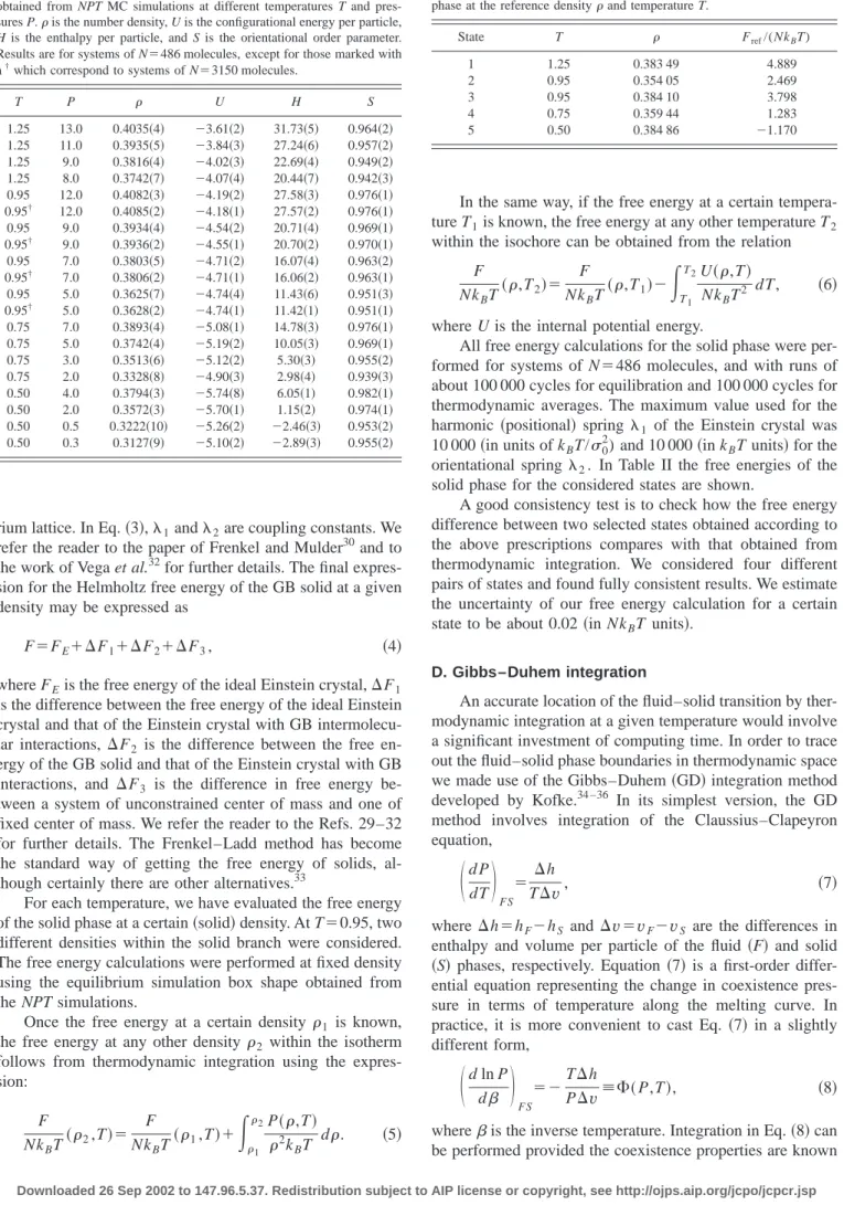
T⫽1.25. As reported in Ref. 12, on compressing the isotro-pic phase at this temperature, the GB fluid undergoes a tran-sition to a nematic phase. Based on free energy calculations, the I – N transition has been shown to take place at PIN

⫽5.20.12 The corresponding solid branch of the isotherm was obtained expanding a solid configuration at high pres-sure ( P⫽13.0). The solid phase was found to be mechani-cally stable up to P⫽5.5. Below this pressure, the solid melted into the nematic phase. Results for some solid state points at T⫽1.25 have been included in Table I. The free energy of the solid phase was computed according to the procedure described in the previous section. By solving the equilibrium conditions, the N – S transition was found to take place at PNS⫽7.68. The behavior of the GB fluid along the

isotherm T⫽1.25 is shown in Fig. 1.

At the next temperature considered here (T⫽0.95) the

I – N nematic transition was located at PIN⫽3.31 from free

energy calculations. As reported by de Miguel,12the nematic phase is mechanically stable upon compression up to P ⫽4.90. Beyond this pressure, the nematic phase transforms 共very slowly兲into a higher density phase with a high degree

TABLE III. Details of the different series of GD integrations performed in the present work to study the fluid–solid coexistence of the GB model. The second column indicates the temperature on the coexistence line used to start the GD integration in the corresponding temperature range共third col-umn兲. The last column indicates the nature of the fluid phase共isotropic or nematic兲in coexistence with the solid phase in each series.

Series Starting T

Temperature range

Integration direction

Observed F – S coexistence

(6)

of translational order. Although with some caveats, this phase was considered to be a SmB. We shall come to this point later.

The simulation of the solid phase at T⫽0.95 was started at P⫽13.0. The solid was subsequently expanded up to P ⫽2.5. At this pressure, the solid melted directly into an iso-tropic fluid: no nematic behavior was found upon expanding the solid phase. Nonetheless, after calculating the free energy of the solid phase, and using the free energy of the nematic and isotropic phases, it was found that the solid–nematic transition takes place before the solid melts into the isotropic fluid. According to our calculations, it follows that PNS

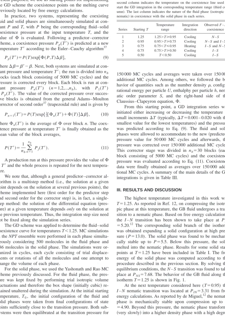
⫽3.64. Thus, the nematic phase is thermodynamically stable at this temperature, although over a narrow range of pres-sures共or densities兲. Figure 2 shows the behavior of the GB fluid at T⫽0.95. The simulation results for the SmB phase reported by de Miguel12 have been included in Fig. 2 for comparison. As can be seen in the figure, the differences between the solid and the SmB densities at a given pressure are small, and we believe that these SmB states correspond, in fact, to quasicrystalline共or imperfect solid兲structures re-sulting from compressing the共nematic兲fluid.

At temperature T⫽0.75 the I – N transition was located at PIN⫽2.06 from free energy calculations

12

and the nematic phase was found to be mechanically stable up to P⫽2.20. At this pressure, the nematic phase is driven upon compression to a layered phase identified as SmB in Ref. 12. The solid phase at T⫽0.75 was simulated starting from P⫽7.0 The resulting equilibrated configuration was slowly expanded in small pressure steps up to P⫽1.25. Below this pressure, the solid phase melted into the isotropic phase. As observed for

T⫽0.95, no intermediate nematic phase was formed on ex-panding the solid phase. Interesting enough, the I – N transi-tion is pre-empted at this temperature by freezing, which occurs, according to the free energy calculations of the present work, at PIS⫽1.85. Hence, for T⫽0.75, the nematic

phase is not thermodynamically stable. The simulation re-sults for the GB fluid at T⫽0.75 are shown in Fig. 2. Also

shown in the figure are the results for the SmB phase in the compression runs reported by de Miguel,12the resulting den-sities falling on top of the solid branch of the isotherm. This gives further evidence to the fact that the reported SmB phase seems to correspond to a crystal structure.

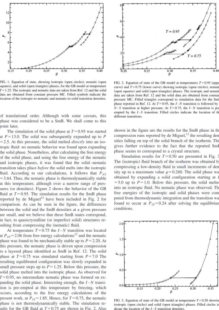
Simulation results for T⫽0.50 are presented in Fig. 3. The共isotropic兲fluid branch of the isotherm was obtained by compressing a low-density fluid in small increments of den-sity up to a maximum value ␳⫽0.260. The solid phase was obtained by expanding a solid configuration starting at P ⫽5.0 up to P⫽1.0. Below this pressure, the solid melted into an isotropic fluid. No nematic phase was observed. The free energies of the isotropic and solid phases were com-puted from thermodynamic integration and the transition was found to occur at PIS⫽0.24 after solving the equilibrium

conditions. FIG. 1. Equation of state, showing isotropic共open circles兲, nematic共open

squares兲, and solid共open triangles兲phases, for the GB model at temperature

T⫽1.25. The isotropic and nematic data are taken from Ref. 12 and the solid data are obtained from constant pressure MC. Filled symbols indicate the location of the isotropic-to-nematic and nematic-to-solid transition densities.

FIG. 2. Equation of state of the GB model at temperatures T⫽0.95共upper curve兲and T⫽0.75共lower curve兲showing isotropic共open circles兲, nematic 共open squares兲and solid共open triangles兲phases. The isotropic and nematic data are taken from Ref. 12 and the solid data are obtained from constant pressure MC. Filled triangles correspond to simulation data for the SmB phase reported in Ref. 12. At T⫽0.95, the I – N transition is followed by a

N – S transition at higher pressure. At T⫽0.75, the I – N transition is pre-empted by the I – S transition. Filled circles indicate the location of the different transitions.

(7)

A summary of the thermodynamic properties at the fluid–solid transition is given in Table IV.

The simulations in the high density region reported above provided no indication of a transition to a SmB liquid as the solid phase was expanded. For systems of soft parallel spherocylinders, however, simulations give evidence of a crystal-to-SmB transition that involves a significant volume change at the transition.38,39For the GB system we could not detect any density or enthalpy discontinuity on the equation of state. Although this transition is expected to be first order on the basis of symmetry arguments,20,21 it could be very weak for GB systems and therefore difficult to observe. Stronger evidence of the absence 共or presence兲of an inter-mediate SmB phase may be obtained by measuring the in-layer pair distribution function g_⬜(r_⬜). This function mea-sures positional correlations of the molecules within each single layer and so should allow to distinguish between a smectic phase关expected in-plane liquidlike behavior with no long range structure in g_⬜(r_⬜)] and a true crystal phase. In order to get the behavior of g_⬜(r_⬜) at longer distances, this function was evaluated for substantially larger systems with

N⫽3150 共six layers, each layer consisting of 525 mol-ecules兲. g_⬜(r_⬜) was obtained along the solid branch of the isotherm T⫽0.95, expanding the system from P⫽25.0 in small pressure steps up to a pressure at which the system melted into the nematic phase. Again, no indications were found of any additional transition implying two-dimensional melting of crystal layers. As the crystal phase was expanded,

g_⬜(r_⬜) exhibited considerable structure, with well-resolved peaks, the only observable effect being a slight broadening of the peaks and a decrease in the intensity of the first few peaks. Figure 4 illustrates g_⬜(r_⬜) for selected state points. At all pressures, the behavior of g_⬜(r_⬜) indicated clear crystal-line order. The results presented here seem to confirm that the high-density SmB phase reported in previous studies for the GB fluid is in fact a molecular solid and is not a smectic liquid crystal phase.

In order to calculate the complete melting curve for tem-peratures T⬍1.25 we used GD integration. In principle, the implementation of the method requires knowledge of one single point on the coexistence curve as the initial starting point. Obviously, the coexistence properties will be subject to errors due 共among other factors兲 to the finite integration

step size used for the numerical integration of Eq.共8兲. These errors are expected to become larger as the integration pro-ceeds, and may be particularly significant if the temperature range under investigation is wide. Thus, in order to minimize these propagation-of-error effects, we decided to use differ-ent starting points 共particularly, those points obtained from the free energy calculations reported above兲to cover differ-ent temperature ranges共see Table III兲.

The first series was started at T⫽1.25 and the tempera-ture was decreased up to T⫽0.95 using a temperature step of 0.02. The corresponding results in the temperature-density and pressure–temperature diagram are shown in Figs. 5 and 6, respectively. As expected, the fluid phase in coexistence with the solid phase was found to exhibit nematic behavior in this range of temperatures. The N – S transition properties for the lowest temperature in this range (T⫽0.95) have been included in Table IV. According to the results included in

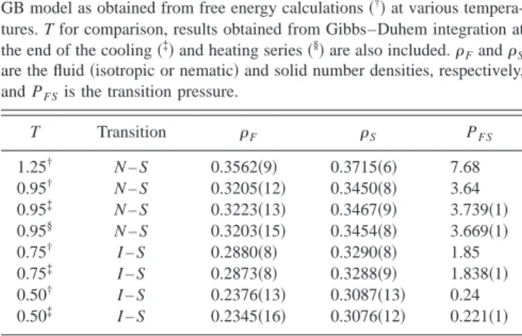
TABLE IV. Thermodynamic properties at the fluid–solid transition for the GB model as obtained from free energy calculations共†_兲_{at various}

tempera-tures. T for comparison, results obtained from Gibbs–Duhem integration at the end of the cooling共‡兲and heating series共§兲are also included.␳Fand␳S

are the fluid共isotropic or nematic兲and solid number densities, respectively, and PFSis the transition pressure.

T Transition ␳F ␳S PFS

1.25† N – S 0.3562共9兲 0.3715共6兲 7.68 0.95† N – S 0.3205共12兲 0.3450共8兲 3.64 0.95‡ N – S 0.3223共13兲 0.3467共9兲 3.739共1兲 0.95§ N – S 0.3203共15兲 0.3454共8兲 3.669共1兲 0.75† I – S 0.2880共8兲 0.3290共8兲 1.85 0.75‡ I – S 0.2873共8兲 0.3288共9兲 1.838共1兲 0.50† I – S 0.2376共13兲 0.3087共13兲 0.24 0.50‡ I – S 0.2345共16兲 0.3076共12兲 0.221共1兲

FIG. 4. Two-dimensional in-plane positional correlation function g_⬜(r_⬜) as obtained from constant pressure MC simulation for systems of 3150 GB particles at T⫽0.95 and different pressure values P. Each curve corre-sponds, from top to bottom, to P⫽20, 12, 8, and 5. The zero of g_⬜(r_⬜) has been shifted on the vertical scale for clarity.

(8)

this table, the transition properties obtained by GD integra-tion compare reasonably well with those obtained by free energy calculations.

A second series of GD integration was designed to trace out the fluid–solid coexistence curve for temperatures 0.75 ⭐T⭐0.95. We recall that, according to the free energy cal-culations reported above, the fluid phase in coexistence with the solid is nematic at T⫽0.95 and isotropic at T⫽0.75. Therefore, a nematic-to-isotropic transition is expected to take place in the fluid subsystem at some intermediate tem-perature. Starting from T⫽0.95, the temperature was re-duced in steps of 0.01 up to T⫽0.75. The resulting coexist-ence densities and pressures are shown in Figs. 5 and 6. The corresponding values at the lowest temperature (T⫽0.75) have been included in Table IV and compared with those obtained from free energy calculations. Both procedures yield fully consistent results. Following the behavior of the nematic order parameter, the nematic-to-isotropic transition was observed to take place at T⬇0.85. Also, as expected, this transition is accompanied by a small density jump, as can be observed in Fig. 5.

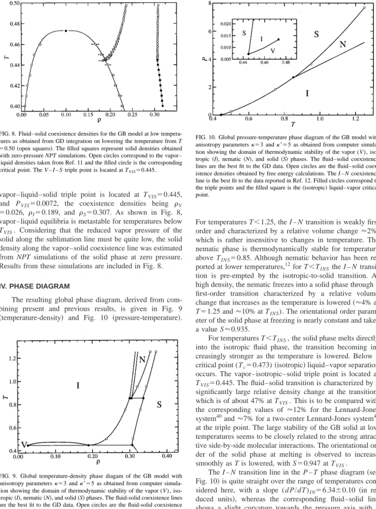
We should note that the use of the GD scheme requires the integration path be reversible. This may cast doubt on the reliability of the GD integration through the N – I transition occurring at T⬇0.85. We have attempted to check this issue by integrating up in temperature along the coexistence curve starting from T⫽0.75 in temperature steps of 0.01 up to T ⫽0.95. Values of the coexistence densities at the fluid–solid transition resulting from integration up and down in this range of temperatures are shown in Fig. 7. In the heating series, the I – N transition takes place at T⬇0.85 and no sig-nificant hysteresis effects are observed at the transition. At the final temperature along this heating sequence (T ⫽0.95), the GD integration yields a transition pressure

PNS⫽3.669(1) which is in fairly good agreement with the

value PNS⫽3.64 obtained by thermodynamic integration and

used as a starting point for the cooling sequence. From the results given in Fig. 7, we conclude that the GD integration

path through the I – N – S triple point is reversible. A similar conclusion was reported for the I – N transition ocurring along the vapor–liquid line for other parametrizations of the GB model.11 From the present results, the I – N – S triple point is located at TINS⫽0.85 and PINS⫽2.70, the

coexist-ence densities being ␳I⫽0.300, ␳N⫽0.305, and ␳S⫽0.337,

for the isotropic, nematic, and solid phases, respectively. A new series of GD integration was started at T⫽0.75 from the corresponding coexistence data obtained previously by free energy calculations, and the integration was extended up to T⫽0.50. The integration proceeded in temperature steps of 0.01, although the step size was reduced to 0.005 for temperatures T⬍0.60. The fluid–solid transition properties obtained along this sequence are shown in Figs. 5 and 6 and the resulting pressure and densities at the lowest temperature (T⫽0.50) are presented in Table IV. The transition pressure obtained by GD integration ( PIS⫽0.221) is slightly lower

than the value obtained from thermodynamic integration ( PIS⫽0.24).

The last GD integration series was initiated at T⫽0.50 and continued to lower temperatures. According to previous investigations, the GB fluid shows vapor–liquid separation in this region. In principle, integration of Eq. 共8兲may give rise to numerical unstabilities in this temperature range. This is because the transition pressure approaches zero as the tem-perature is lowered, and the right-hand side of Eq. 共8兲 may grow quite large. The integration in this temperature range was then performed using Eq.共7兲with an integration step of 0.0025. For temperatures T⬍0.450, the integration step was reduced to 0.001. Results are presented in Fig. 8. Results for the vapor–liquid equilibria as obtained from Gibbs ensemble simulations11 are also shown in the figure. From these data, the 共vapor–liquid兲 critical point is located at Tc

⫽0.473(10), Pc⫽0.0134(9), the critical density being ␳c

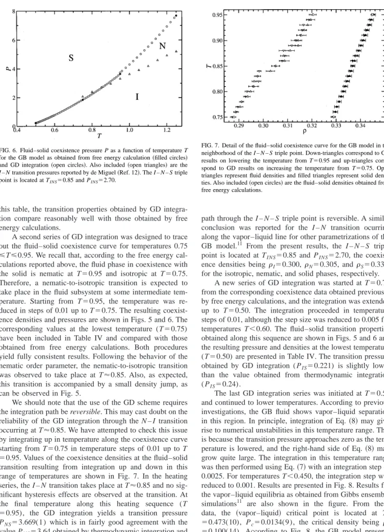
⫽0.100(14). According to Fig. 8, the GB model presents vapor–liquid separation over an unexpectedly narrow range of temperatures. Combining all the simulation data, the FIG. 6. Fluid–solid coexistence pressure P as a function of temperature T

for the GB model as obtained from free energy calculation共filled circles兲 and GD integration共open circles兲. Also included共open triangles兲are the

I – N transition pressures reported by de Miguel共Ref. 12兲. The I – N – S triple point is located at TINS⫽0.85 and PINS⫽2.70.

(9)

vapor–liquid–solid triple point is located at TVIS⫽0.445,

and PVIS⫽0.0072, the coexistence densities being ␳V

⫽0.026, ␳I⫽0.189, and ␳S⫽0.307. As shown in Fig. 8,

vapor–liquid equilibria is metastable for temperatures below

TVIS. Considering that the reduced vapor pressure of the

solid along the sublimation line must be quite low, the solid density along the vapor–solid coexistence line was estimated from NPT simulations of the solid phase at zero pressure. Results from these simulations are included in Fig. 8.

IV. PHASE DIAGRAM

The resulting global phase diagram, derived from com-bining present and previous results, is given in Fig. 9 共temperature-density兲 and Fig. 10 共pressure-temperature兲.

For temperatures T⬍1.25, the I – N transition is weakly first order and characterized by a relative volume change ⬇2%, which is rather insensitive to changes in temperature. The nematic phase is thermodynamically stable for temperature above TINS⫽0.85. Although nematic behavior has been

re-ported at lower temperatures,12for T⬍TINS the I – N

transi-tion is pre-empted by the isotropic-to-solid transitransi-tion. At high density, the nematic freezes into a solid phase through a first-order transition characterized by a relative volume change that increases as the temperature is lowered共⬇4% at

T⫽1.25 and⬇10% at TINS). The orientational order

param-eter of the solid phase at freezing is nearly constant and takes a value S⬇0.935.

For temperatures T⬍TINS, the solid phase melts directly

into the isotropic fluid phase, the transition becoming in-creasingly stronger as the temperature is lowered. Below a critical point (Tc⫽0.473)共isotropic兲liquid–vapor separation

occurs. The vapor–isotropic–solid triple point is located at

TVIS⫽0.445. The fluid–solid transition is characterized by a

significantly large relative density change at the transition, which is of about 47% at TVIS. This is to be compared with

the corresponding values of ⬇12% for the Lennard-Jones system40and⬇7% for a two-center Lennard-Jones system41 at the triple point. The large stability of the GB solid at low temperatures seems to be closely related to the strong attrac-tive side-by-side molecular interactions. The orientational or-der of the solid phase at melting is observed to increase smoothly as T is lowered, with S⫽0.947 at TVIS.

The I – N transition line in the P – T phase diagram共see Fig. 10兲is quite straight over the range of temperatures con-sidered here, with a slope (d P/dT)IN⫽6.34⫾0.10 共in

re-duced units兲, whereas the corresponding fluid–solid line shows a slight curvature towards the pressure axis with a slope (d P/dT)FS⫽9.17⫾0.17 at TINS.

No evidence of smecticlike ordering has been found at FIG. 8. Fluid–solid coexistence densities for the GB model at low

tempera-tures as obtained from GD integration on lowering the temperature from T ⫽0.50共open squares兲. The filled squares represent solid densities obtained with zero-pressure NPT simulations. Open circles correspond to the vapor– liquid densities taken from Ref. 11 and the filled circle is the corresponding critical point. The V – I – S triple point is located at TVIS⫽0.445.

FIG. 9. Global temperature-density phase diagam of the GB model with anisotropy parameters␬⫽3 and␬⬘⫽5 as obtained from computer simula-tion showing the domain of thermodynamic stability of the vapor (V), iso-tropic共I兲, nematic共N兲, and solid共S兲phases. The fluid-solid coexistence lines are the best fit to the GD data. Open circles are the fluid-solid coexistence densities obtained by free energy calculations. The I – N coexistence lines are the best fit to the data reported in Ref. 12. Filled symbols correspond to the coexistence densities at the triple points.

(10)

any of the temperatures investigated in this work. The present results suggest 共1兲 the GB model does not exhibit SmB phase共at least, for this combination of parameters兲; and 共2兲 the high-density phase, designated SmB in previous simulation studies,6,9,12 corresponds to a crystal phase. As this phase resulted from compressing a translationally disor-dered fluid 共at constant volume or at constant pressure兲the crystalline order was incomplete. Therefore, it seems that the strong lateral attractive interactions present in the model tend to stabilize a layered structure, although the structure is crys-talline.

ACKNOWLEDGMENTS

This work was financed by the Spanish DGI共Direccio´n General de Investigacio´n兲 under Projects Nos. BFM2001-1420-C02-02 and BFM2001-1420-C02-01.

1

Structure of Liquid Crystals, edited by P. S. Pershan共World Scientific, New York, 1988兲.

2_{P. G. de Gennes and J. Prost, The Physics of Liquid Crystals, 2nd ed.} 共Clarendon, Oxford, 1993兲.

3

Physical Properties of Liquid Crystals, edited by D. Demus et al.共 Wiley-VCH, New York, 1999兲.

4_{See, for example, M. P. Allen, in Advances in the Computer Simulations of}

Liquid Crystals, edited by P. Pasini and C. Zannoni共Kluwer, Dordrecht, 2000兲.

5

J. G. Gay and B. J. Berne, J. Chem. Phys. 74, 3316共1981兲.

6_{G. R. Luckhurst, R. A. Stephens, and R. W. Phippen, Liq. Cryst. 8, 451} 共1990兲.

7_{E. de Miguel, L. F. Rull, M. K. Chalam, and K. E. Gubbins, Mol. Phys.}

71, 1223共1990兲.

8

E. de Miguel, L. F. Rull, M. K. Chalam, K. E. Gubbins, and F. van Swol, Mol. Phys. 72, 593共1991兲.

9_{E. de Miguel, L. F. Rull, M. K. Chalam, and K. E. Gubbins, Mol. Phys.}

74, 405共1991兲.

10

R. Hashim, G. R. Luckhurst, and S. Romano, J. Chem. Soc., Faraday Trans. 91, 2141共1995兲.

11_{E. de Miguel, E. Martı´n del Rı´o, J. T. Brown, and M. P. Allen, J. Chem.}

Phys. 105, 4234共1996兲.

12_{E. de Miguel, Mol. Phys. 100, 2449}_共₂₀₀₂_兲_.

13_{E. Velasco, A. M. Somoza, and L. Mederos, J. Chem. Phys. 102, 8107} 共1995兲.

14_{E. Velasco and L. Mederos, J. Chem. Phys. 109, 2361}_共₁₉₉₈_兲_. 15_{G. R. Luckhurst and P. S. J. Simmonds, Mol. Phys. 80, 233}_共₁₉₉₃_兲_. 16

M. P. Allen, J. T. Brown, and M. A. Warren, J. Phys.: Condens. Matter 8, 9433共1996兲.

17_{J. T. Brown, M. P. Allen, E. Martı´n del Rı´o, and E. de Miguel, Phys. Rev.}

E 57, 6685共1998兲.

18_{M. A. Bates and G. R. Luckhurst, J. Chem. Phys. 110, 7087}_共₁₉₉₉_兲_. 19_{J. W. Goodby and G. W. Gray, in Physical Properties of Liquid Crystals,}

edited by D. Demus et al.共Wiley-VCH, New York, 1999兲, Chap. 2.

20_{C. C. Huang and T. Stoebe, Adv. Phys. 42, 343}_共₁₉₉₃_兲_. 21_{K. J. Strandburg, Rev. Mod. Phys. 60, 161}_共₁₉₈₈_兲_.

22_{R. J. Birgenau and J. D. Litster, J. Phys.}_共_Paris_兲_{39, L399}_共₁₉₇₈_兲_. 23_{B. I. Halperin and D. R. Nelson, Phys. Rev. Lett. 41, 121}_共₁₉₇₈_兲_. 24_{R. Pindak, D. E. Moncton, S. C. Davey, and J. W. Goodby, Phys. Rev.}