Extending Wertheim’s perturbation theory to the solid phase
of Lennard-Jones chains: Determination of the global phase diagram
C. Vega
Departamento de Quı´mica Fı´sica, Facultad de Ciencias Quı´micas, Universidad Complutense, 28040 Madrid, Spain
F. J. Blas
Departamento de Fı´sica Aplicada, Escuela Polite´cnica Superior, Universidad de Huelva, 21819 La Ra´bida, Huelva, Spain
A. Galindo
Department of Chemical Engineering and Chemical Technology, Imperial College of Science, Technology and Medicine, Prince Consort Road, London SW7 2BY, United Kingdom
共Received 6 November 2001; accepted 6 February 2002兲
Wertheim’s first order thermodynamic perturbation theory共TPT1兲 关M. S. Wertheim, J. Chem. Phys.
87, 7323 共1987兲兴 is extended to model the solid phase of chains whose monomers interact via a Lennard-Jones potential. Such an extension requires the free energy and contact values of the radial distribution function for the Lennard-Jones reference system in the solid phase. Computer simulations have been performed to determine the structural properties of the monomer Lennard-Jones system in the solid phase for a broad range of temperatures and densities. Computer simulations of dimer Lennard-Jones molecules in the solid phase have also been carried out. The theoretical results for the equation of state, the internal energy, and the sublimation curve of the dimer model in the solid phase are in excellent agreement with the simulation data. The extended theory is used to determine the global共solid–liquid–vapor兲phase diagram of the LJ dimer model; the theoretical estimate of the triple point temperature for the LJ dimer is T*⫽0.653. Similarly, Wertheim’s TPT1 is used to determine the global phase diagram of chains formed by up to 8 monomer units. It is found that the calculated triple point temperature is hardly affected by the chain length, and that for large chain lengths the fluid–solid equilibrium coexistence densities are virtually independent of the number of monomers in the chain when the densities are expressed in monomer units. This is in agreement with experimental indications observed in polyethylene, where both the critical and the triple point temperatures tend to finite values for large molecular weights. © 2002 American Institute of Physics. 关DOI: 10.1063/1.1465397兴
I. INTRODUCTION
In the mid-1980s Wertheim presented a very successful theory to study the thermodynamic properties of hard-core fluids interacting via short-range attractive 共association兲 forces,1– 4 such as hydrogen bonding fluids. In this model, when the association strength becomes infinitely strong chains are formed from a fluid of associating monomers.5In this way it is possible to derive an equation of state for a chain of freely-jointed tangent hard segments using only thermodynamic information of the monomer reference fluid. In the simplest implementation of the theory, which is com-monly denoted as the first order thermodynamic perturbation theory 共TPT1兲, the only information required in order to build an approximate equation of state for the chain fluid is the equation of state of the monomer fluid and its pair cor-relation function at contact. The equation of state共EOS兲
aris-ing from TPT1 was proposed independently by Wertheim6
and by Chapman, Jackson, and Gubbins.7In the early 1990s Chapman8showed that Wertheim’s formalism could also be applied to systems with attractive 共dispersion兲 forces. The work of Johnson et al.9,10has shown that Wertheim’s formal-ism yields a good description of the Lennard-Jones 共LJ兲
chain fluid, provided that the EOS and pair correlation func-tion of the reference LJ fluid are accurately known. The same is true for chains formed from monomers interacting via other pair potentials, for instance, the square well potential11 and the Yukawa potential12 have also been incorporated in this context. Therefore, an approximate but reliable descrip-tion of the fluid phase of fully flexible chains 共i.e., with no constraint in the bonding angle or torsional state兲 can be obtained nowadays in a rather straightforward way. The TPT1 theory of Wertheim provides reasonable predictions of the vapor–liquid equilibria for a number of different types of chain.13–16Notice that other theoretical treatments are also succesfull for LJ chains.17
In order to obtain the global phase diagram of flexible chains, the solid phase should also be considered so that fluid–solid coexistence is adequately located within the phase diagram of the model. In the last decade the fluid– solid equilibrium of a number of molecular models have been considered, for example, hard dumbbells, quadrupolar hard dumbbells, hard spherocylinders, hard ionic systems, benzenelike models, and others共see, for instance, the recent review of Monson and Kofke18兲. However, efforts
consider-7645
ing the fluid–solid equilibrium of flexible chains are scarce.
Malanoski and Monson19 have determined via computer
simulation the fluid–solid equilibrium of freely jointed hard sphere chains, and of a hard model of n-alkane molecules.20 Polson and Frenkel21 have determined the fluid–solid equi-libria of LJ chains 共with a bending potential兲 and of a LJ model of n-alkane molecules.22Theoretical works describing the phase equilibria of flexible chains in the solid phase are even more scarce, the work of Sear and Jackson,23 and of Malanoski et al.,24in which the the cell theory is extended to study the solid phase of these molecules, are the exception.
Solid phases of long flexible molecules are of interest since it is at room temperature and pressure that these mol-ecules exhibit the solid phase. For instance, all linear alkanes with more than 20 carbon atoms are solids at room tempera-ture and pressure, and the same is true for polyethylene.25In many industrial processes one has to deal with the fluid– solid separation of alkane mixtures. A theoretical description of the solid phase of flexible chain molecules would be of great interest both from a fundamental and from a practical point of view. Taking into account the success of Wertheim’s TPT1 approach in modelling the fluid phase of chain mol-ecules one is tempted to raise the following question: can the approach be extended to describe the solid phase of flexible
chains? Recently Vega and MacDowell26 have shown that
Wertheim’s TPT1 can be extended to the solid phase of freely jointed hard spheres obtaining excellent agreement with the simulation results of Malanoski and Monson.19The theory is also able to describe the solid phase of two-dimensional freely jointed discs.27 Although chains formed by hard spheres are of interest, it would certainly be more interesting to consider the case of chains formed by Lennard-Jones monomers. Due to the presence of attractive forces, the Lennard-Jones model exhibits vapor–liquid equilibria in ad-dition to the fluid–solid equilibrium, and is therefore of greater practical interest. The goal of this paper is to extend Wertheim’s theory to the solid phase of freely jointed LJ molecules and to provide a first estimate of the global phase diagram of these systems.
Let us briefly discuss the solid structure of freely-jointed chains. In a freely jointed chain there is neither bending nor torsional potentials between the monomers of the chain 共 al-though there is an intramolecular pair interaction between monomers of the same chain separated by more than one bond兲. Therefore there is no energetic penalty when the at-oms of the chains adopt a close-packed structure 共for in-stance the face centered cubic fcc close-packed structure兲 with an ordered arrangement of atoms but with no long-range orientational order in the bond vectors of the chains. Wojciechowski et al.28,29were the first to realize this impor-tant feature in a continuum hard two-dimensional model. In fact Wojciechowski et al.28,29 showed that the stable solid structure of tangent hard-disc dimers in two dimensions is formed by a close-packed arrangement of atoms with a dis-ordered arrangement of bonds. The same idea holds for hard chains in three dimensions,19 and one may expect that the same would occur for a three-dimensional LJ chain. In a sense this is a clever solution of nature. The molecules achieve the close-packed structure of hard spheres, so that
the density is high, and the system is ordered from the point of view of the atoms but not from the point of view of the molecular bonds. The disorder of bonds means that there is an additional contribution to the entropy of the system aris-ing from the degeneracy of the structure. For this reason the stable solid structure for freely jointed models is one with disordered bonds. The extreme flexibility of freely jointed models makes the existence of such a solid possible. Any reduction of flexibility, such as fixing a bond angle in the model, would make the existence of the closed-packed solid with random bonds impossible, since it is likely that the mo-lecular bonding angle would not be compatible with the angles of an fcc arrangement of atoms. As discussed earlier, in the TPT1 approximation a freely-jointed chain is assumed, hence, the expected structure of its solid phase corresponds to that with the monomer segments arranged in an fcc lattice with random bond orientations. Assuming this structure we have used computer simulations to compare with the theoret-ical calculations.
The scheme of this paper is as follows: In Sec. II the extension of Wertheim’s theory to the solid phase of LJ chains is described. In Sec. III details of the simulations per-formed in this work are given. In Sec. IV the results for the LJ dimer system are presented, and in Sec. V the global phase diagrams of LJ chains are presented.
II. BRIEF DESCRIPTION OF WERTHEIM’S PERTURBATION THEORY
We summarize the main ideas contained within Wer-theim’s theory by following the formulation introduced by Zhou and Stell.30–32Let us assume that we have a certain number, Nref, of spherical monomer particles within a certain volume V at temperature T, and that these particles interact through a spherical pair potential uref(r). In this work the pair potential uref(r) is the Lennard-Jones potential with pa-rametersand⑀. We denote this fluid as the reference fluid and the properties of this reference fluid will be labeled by the superscript ref. Let us also assume that in another con-tainer of volume V and temperature T, we have N⫽Nref/m fully flexible chains of m monomers each. By fully flexible chains we mean chains of m monomers, with a fixed bond length of L⫽, and no other constraints 共i.e., there is no restriction in either bonding angles or in torsional angles兲. Each monomer of a certain chain interacts with all the other monomers in the system 共i.e., in the same molecule or in other molecules with the only exception of the monomer/s to which it is bonded兲with the pair potential uref(r). The chain
system described so far will be denoted as the chain fluid. The Helmholtz free energy of the reference fluid Arefcan be divided into an ideal and a residual part as
Aref
NrefkT⫽ Aideal
ref
NrefkT⫹ Aresidual
ref
NrefkT⫽ln共
ref兲⫺1⫹Aresidual ref
NrefkT, 共1兲
ref-erence fluid and that of a system without intermolecular in-teractions at the same temperature and density.
The free energy of the chain fluid A can also be divided into an ideal and a residual part, so that
A
NkT⫽ Aideal
NkT⫹ Aresidual
NkT ⫽ln共兲⫺1⫹ Aresidual
NkT , 共2兲
where is the reduced number density of chains 共i.e., ⫽N3/V兲. Note that the thermodynamic properties without the superscript ref refer to the chain fluid. In addition to the reduced number density of chains, the reduced number den-sity of monomers in the chain fluid m is defined as m
⫽mN3/V. This density is useful when comparing the prop-erties of chains of different lengths since it seems more ap-propriate to compare them at the same reduced number den-sity of monomers. Following Zhou and Stell, the residual properties of the chain fluid are given, after several approxi-mations, as
Aresidual
NkT ⫽m
Aresidualref
NrefkT⫺共m⫺1兲ln y
ref共兲, 共3兲
where yref() is the background correlation function33of the reference共monomer兲fluid at contact length. The background correlation function is related to the pair correlation function gref(r) by
yref共r兲⫽exp共uref共r兲兲gref共r兲, 共4兲
where ⫽1/(kT). Since for the LJ potential uref()⫽0, it holds that yref()⫽gref(). Therefore, the free energy of the chain fluid can be written as
A
NkT⫽ln共兲⫺1⫹m Aresidualref
NrefkT⫺共m⫺1兲ln g
ref共兲. 共5兲
The above equation shows that the free energy of the chain fluid may be obtained from a knowledge of the re-sidual free energy of the reference fluid and the pair back-ground correlation function of the reference fluid at the bonding distance of the monomers in the chain. The equation of state which follows from Eq.共5兲is given by
Z⫽mZref⫺共m⫺1兲
冉
1⫹refln gref共兲
ref
冊
, 共6兲where we have defined Zref as Zref⫽pref/(refkT). The re-sidual part of the internal energy U is given by
U
NkT⫽m Uref
NrefkT⫹共m⫺1兲T
冉
ln gref共兲
T
冊
. 共7兲We denote Eqs. 共5兲, 共6兲, and 共7兲 as Wertheim’s TPT1 theory, noting that the arguments used to arrive to Eqs.共5兲, 共6兲, and共7兲make no special mention as to the actual nature 共i.e., fluid or solid兲of the phase considered.30,32We suggest the use of these two equations for both the fluid phase and the solid phase. All that is then needed in order to obtain a unified theory for the phase equilibria of chain molecules is the residual free energy, compressibility factor and pair cor-relation function of the monomer system both in the fluid and the solid phase. Johnson et al.9,10 have provided values of the free energy, and the structural properties 关i.e.,
gfluidref ()兴of the monomer LJ fluid. In this work we use their implementation of the TPT1 approach9,10 in what relates to the fluid phases. Van der Hoef34 has recently proposed an analytical expression for the free energy of the LJ monomer solid. His analytical expression is essentially a fit to the most recent simulation results for the solid phase of this model. We adopt the expression provided by van der Hoef for the free energy of the LJ monomer solid. The other information required by the theory is the value of gsolidref () for the LJ monomer solid. Since this is not available from previous works we have performed computer simulations of the LJ monomer system in the solid phase in order to obtain gsolidref () for a number of temperatures and densities. The simulation results of gsolidref () were fitted to an empirical expression of the same form as that proposed by Johnson et al. for the fluid phase.10 In order to check the theory we have also performed a number of computer simulations of the LJ dimer system in the solid phase. Details of the simu-lations are given in the following section.
III. SIMULATION DETAILS
A. Computer simulations of the LJ monomer in the solid phase
We have used the canonical ensemble (NVT) Monte Carlo 共MC兲 simulation technique to obtain the pair radial distribution function at contact length in a system of Lennard-Jones spheres in the solid phase. All simulations were carried out for Nref⫽500 particles, with initial configu-rations of particles arranged in cubic close packing. In par-ticular, the Lennard-Jones spheres are arranged on a face-centered cubic or fcc structure.
As corresponds to an NVT Monte Carlo simulation, the number of particles, volume, and temperature are specified a priori, allowing the pressure and internal energy to fluctuate. Attempts to displace a molecule in a random manner are made in order to reach internal equilibrium. Periodic bound-ary conditions and the minimum image convention are also used. The calculation of the configurational internal energy is performed in the usual way by truncating the Lennard-Jones interactions at a distance rc⫽3, and the pressure is ob-tained using the virial equation.35The total internal configu-rational energy and pressure are recovered by adding back the standard long-range corrections. The pair radial distribu-tion funcdistribu-tion is calculated using the standard procedure35 with a grid space ⌬r⫽0.01. Such a fine grid is required since gsolidref () changes significantly in the proximities of, and this effect is especially important in the solid phase. The total simulation length is set to 200 000 cycles, with 50 000 equilibration cycles and 150 000 averaging cycles. Each cycle consists of Nrefattempted particle displacements. The errors are estimated by dividing the simulation in blocks of 10 000 cycles, so as to obtain statistically-independent block sequences, and calculating the standard errors of the mean.
⫽p3/⑀. In the Lennard-Jones共LJ兲monomer reference fluid the reduced number density is denotedref共we suppress the superscript*in order to keep the notation as simple as pos-sible兲, and it is defined asref⫽Nref3/V.
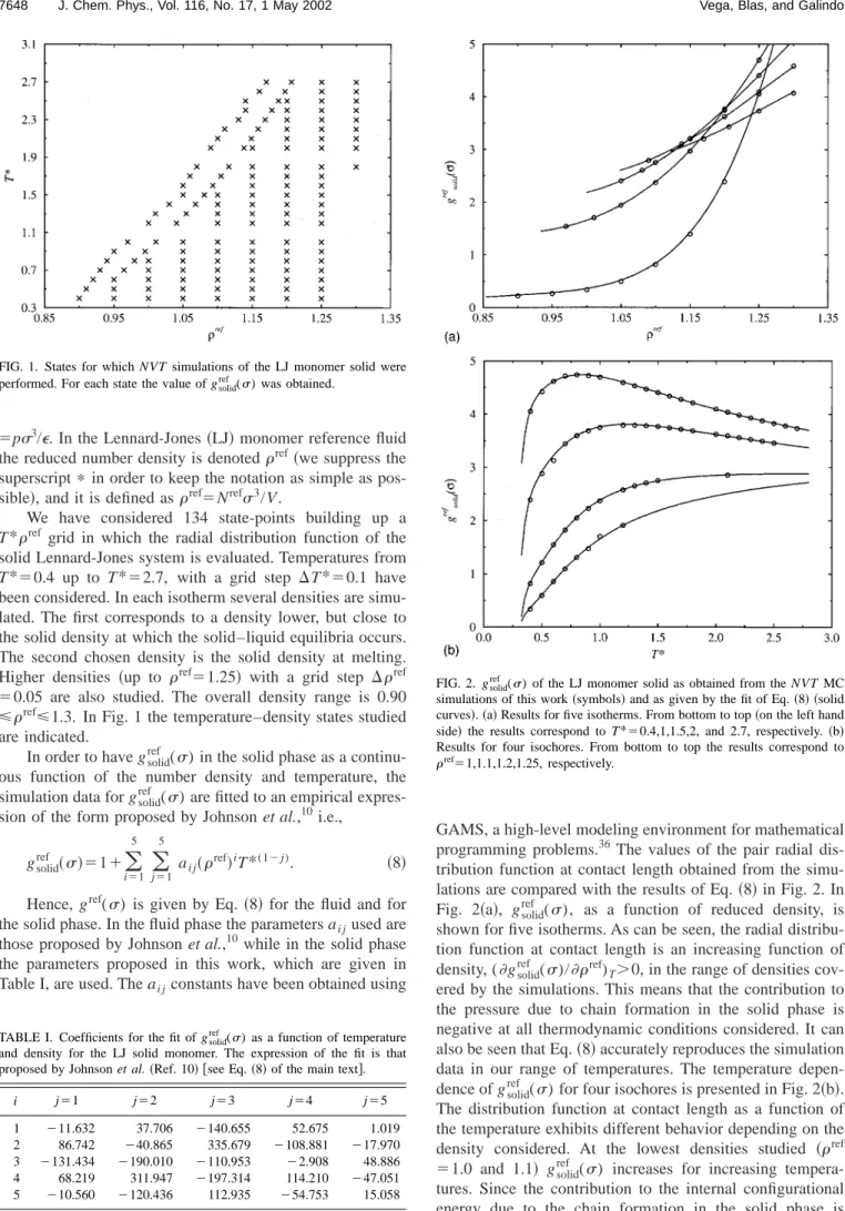
We have considered 134 state-points building up a T*ref grid in which the radial distribution function of the
solid Lennard-Jones system is evaluated. Temperatures from T*⫽0.4 up to T*⫽2.7, with a grid step ⌬T*⫽0.1 have been considered. In each isotherm several densities are simu-lated. The first corresponds to a density lower, but close to the solid density at which the solid–liquid equilibria occurs. The second chosen density is the solid density at melting. Higher densities 共up to ref⫽1.25兲 with a grid step ⌬ref ⫽0.05 are also studied. The overall density range is 0.90 ⭐ref⭐1.3. In Fig. 1 the temperature–density states studied
are indicated.
In order to have gsolidref () in the solid phase as a continu-ous function of the number density and temperature, the simulation data for gsolidref () are fitted to an empirical expres-sion of the form proposed by Johnson et al.,10 i.e.,
gsolidref 共兲⫽1⫹
兺
i⫽1 5
兺
j⫽1 5
ai j共ref兲iT*(1⫺j). 共8兲
Hence, gref() is given by Eq. 共8兲 for the fluid and for the solid phase. In the fluid phase the parameters ai jused are
those proposed by Johnson et al.,10 while in the solid phase the parameters proposed in this work, which are given in Table I, are used. The ai jconstants have been obtained using
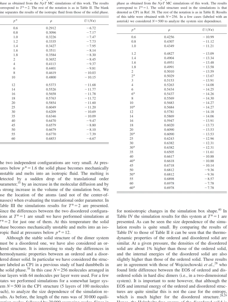
GAMS, a high-level modeling environment for mathematical programming problems.36 The values of the pair radial dis-tribution function at contact length obtained from the simu-lations are compared with the results of Eq.共8兲in Fig. 2. In Fig. 2共a兲, gsolidref (), as a function of reduced density, is shown for five isotherms. As can be seen, the radial distribu-tion funcdistribu-tion at contact length is an increasing funcdistribu-tion of density, (gsolidref ()/ref)T⬎0, in the range of densities
cov-ered by the simulations. This means that the contribution to the pressure due to chain formation in the solid phase is negative at all thermodynamic conditions considered. It can also be seen that Eq.共8兲accurately reproduces the simulation data in our range of temperatures. The temperature depen-dence of gsolidref () for four isochores is presented in Fig. 2共b兲. The distribution function at contact length as a function of the temperature exhibits different behavior depending on the density considered. At the lowest densities studied 共ref ⫽1.0 and 1.1兲 gsolidref () increases for increasing tempera-tures. Since the contribution to the internal configurational energy due to the chain formation in the solid phase is FIG. 1. States for which NVT simulations of the LJ monomer solid were
performed. For each state the value of gsolidref () was obtained.
TABLE I. Coefficients for the fit of gsolidref () as a function of temperature and density for the LJ solid monomer. The expression of the fit is that proposed by Johnson et al.共Ref. 10兲 关see Eq.共8兲of the main text兴.
i j⫽1 j⫽2 j⫽3 j⫽4 j⫽5
1 ⫺11.632 37.706 ⫺140.655 52.675 1.019
2 86.742 ⫺40.865 335.679 ⫺108.881 ⫺17.970
3 ⫺131.434 ⫺190.010 ⫺110.953 ⫺2.908 48.886
4 68.219 311.947 ⫺197.314 114.210 ⫺47.051
5 ⫺10.560 ⫺120.436 112.935 ⫺54.753 15.058
FIG. 2. gsolid ref
() of the LJ monomer solid as obtained from the NVT MC simulations of this work共symbols兲and as given by the fit of Eq.共8兲 共solid curves兲.共a兲Results for five isotherms. From bottom to top共on the left hand side兲the results correspond to T*⫽0.4,1,1.5,2, and 2.7, respectively. 共b兲 Results for four isochores. From bottom to top the results correspond to
closely related with the first derivative of gsolidref () with re-spect to the temperature共at constant density兲, this contribu-tion is positive at the lowest densities. At higher densities 共ref⫽1.2 toref⫽1.25兲g
solid
ref () shows a more complicated
behavior; at low temperatures it behaves as an increasing function of the temperature, a maximum is observed at inter-mediate temperatures, and at the highest temperatures it turns to a decreasing behavior. In summary, the contribution to the internal configurational energy due to the chain formation in the solid phase is negative at high temperatures and densi-ties, and positive for all other thermodynamic conditions considered in our study.
B. Computer simulations of the LJ dimer in the solid phase
In order to test the proposed theory we have performed N pT Monte Carlo simulations of LJ dimer molecules in the solid phase. The reduced bond length of the dimer is L* ⫽L/⫽1, where L is the bond length. In the Monte Carlo run three different types of moves were performed: particle translations, particle rotations, and volume changes. These three types of move leave the bond length unchanged. Notice that the LJ chains considered by Johnson et al.10 in their molecular dynamics study used stiff springs to keep contigu-ous monomers bonded so that in their study the bond length is allowed to fluctuate around the equilibrium value L⫽. In our simulations a typical run consisted of 30 000 equilibra-tion cycles and 30 000 averaging cycles, where a cycle con-sists of a trial move共translation or rotation兲per particle plus an attempt to change the volume of the system. The magni-tude of the displacement of the center of mass, angle of rotation and volume change was controlled to keep the ac-ceptance ratio close to 0.4. Translation and rotation moves were accepted by following the standard Metropolis criterion.35 The site–site LJ potential is truncated at rc
⫽2.5, and the long-range corrections to the internal energy are added as usual by assuming that the site–site pair corre-lation function is equal to one for distances larger than the cutoff value.35 Note that in our N pT simulations the long range correction to the energy was incorporated into the Mar-kov chain共whenever the volume of the system changed兲, so that the output densities are good estimates of the corre-sponding densities of the system without truncation. A num-ber of simulations with rc⫽3 have also been carried out,
finding no significant difference with the densities obtained using rc⫽2.5.
In order to describe a disordered structure, a close-packed faced centered cubic共fcc兲arrangement of atoms was generated and the molecular bonds were randomly distrib-uted. That was done as follows. We generated a cubic hyper-cell by joining together eight face centered cubic unit hyper-cells of atoms. The number of atoms per hypercell is 32 共1 in the vertex, 15 in the faces, 3 in the edges, and 13 inside兲. We connected the 32 atoms randomly, forming 16 dimers. The simulation box was obtained by joining together 27 such hypercells. Therefore the total number of molecules in the N pT MC simulations of the disordered structure was N ⫽432共27 hypercells with 16 dimers each兲. Disordered solid
configurations similar to those considered here, are also found in two-dimensional hard dimer discs28,29,37and in hard sphere chain19 systems. Note also that there is no true close packing for a soft potential such as the LJ but the reduced number density of hard spheres at close packing, i.e., &, provides a good starting point. This disordered structure was expanded to lower densities by performing N pT simulations at successively decreasing pressures. In order to assess the influence of generating different starting random solid con-figurations a second random structure was generated, then carrying out a number of N pT simulations in an identical way. It is important to note that, since the distribution of bonds in the solid phase is assumed isotropic, the scaling in these N pT simulations was done isotropically. In what fol-lows the reduced configurational internal energy will be given as U*⫽U/(N⑀) 共note that N corresponds to the num-ber of molecules, and not the numnum-ber of segments兲. The simulation results in this work were obtained for two iso-therms T*⫽1 and T*⫽2. In Table II the simulation results for the disordered solid phase at T*⫽1 are shown. The re-sults presented are the average of the runs for two indepen-dent disordered configurations. For a number of pressures the typical difference between the properties of the two indepen-dent configurations are indicated in parentheses. As can be seen the differences in thermodynamic properties between TABLE II. Thermodynamic properties of a LJ dimer in a disordered solid phase as obtained from the N pT MC simulations of this work. The results correspond to T*⫽1. The results presented are the arithmetic average of the results for two independent disordered configurations. The reduced pressure is defined as p*⫽p/(⑀/3). The reduced number density of dimers is
de-fined as⫽N3/V. N stands for the number of molecules. The blank line
separates the results of the isotropic fluid from those of the solid phase. For a few states we have presented in parentheses the difference between the results of the two independent disordered configurations.
p* U/(N⑀)
0.6 0.4255 ⫺10.99
0.8 0.4309 ⫺11.12
1.0 0.4353 ⫺11.22
1.2 0.4396 ⫺11.31
1.4 0.4432 ⫺11.39
1.6 0.4973 ⫺13.15
1.8 0.5002 ⫺13.19
2 0.5047 ⫺13.29
3 0.5197共4兲 ⫺13.57(4)
4 0.5314 ⫺13.74
6 0.5490 ⫺13.89
8 0.5626 ⫺13.92
10 0.5738共5兲 ⫺13.88(3)
12 0.5835 ⫺13.78
14 0.5921 ⫺13.65
16 0.6001 ⫺13.49
18 0.6074 ⫺13.30
20 0.6142共3兲 ⫺13.10(3)
25 0.6297 ⫺12.53
30 0.6431 ⫺11.90
35 0.6549 ⫺11.23
40 0.6656 ⫺10.54
45 0.6751共1兲 ⫺9.83(2)
50 0.6838 ⫺9.12
the two independent configurations are very small. At pres-sures below p*⫽1.6 the solid phase becomes mechanically unstable and melts into an isotropic fluid. The melting is detected by a sudden drop of the translational order parameter,35by an increase in the molecular diffusion and by a strong increase in the volume of the simulation box. We use the location of the atoms 共and not of the center-of-masses兲when evaluating the translational order parameter. In Table III the simulations results for T*⫽2 are presented. Since the differences between the two disordered configura-tions at T*⫽1 are small we have performed simulations at T*⫽2 for just one of them. At this temperature the solid phase becomes mechanically unstable and melts into an iso-tropic fluid at pressures below p*⫽12.
Although the stable solid structure of the dimer system must be a disordered one, we have also considered an or-dered structure. It is interesting to study the differences in thermodynamic properties between an ordered and a disor-dered dimer solid. In particular we have considisor-dered the struc-ture labeled as CP1 in a previous study of hard dumbbells in the solid phase.38In this case N⫽256 molecules arranged in four layers with 64 molecules per layer were used. For a few states we performed simulations for a somewhat larger sys-tem N⫽500 in the CP1 structure共5 layers of 100 molecules each兲, to analyze the size dependence of the simulation re-sults. As before, the length of the runs was of 30 000 equili-bration cycles, followed by 30 000 averaging cycles. Since in this case the system is no longer cubic, the Rahman– Parrinello39version of the N pT MC is used in order to allow
for nonisotropic changes in the simulation box shape.40 In Table IV the simulation results for this system at T*⫽1 are presented. As can be seen the size dependence of the simu-lation results is quite small. By comparing the results of Table IV to those of Table II it can be seen that the thermo-dynamic properties of the ordered and disordered solid are similar. At a given pressure, the densities of the disordered solid are about 1% higher than those of the ordered solid, and the internal energies of the disordered solid are also slightly higher than those of the ordered solid. These results are in agreement with those of Wojciechowski et al.,28 who found little difference between the EOS of ordered and dis-ordered solids in hard disc dimers共i.e., in a two-dimensional system兲. It is important to note however, that although the EOS and internal energy of the ordered and disordered struc-tures are quite similar this is not the case for the entropy, which is much higher for the disordered structure.28,29 Hence, the Helmholtz free energy of the disordered solid is significantly lower than that of the ordered solid, so that the equilibrium structure of the LJ dimer in the solid phase cor-TABLE III. Thermodynamic properties of a LJ dimer in a disordered solid
phase as obtained from the N pT MC simulations of this work. The results correspond to T*⫽2. The rest of the notation is as in Table II. The blank line separates the results of the isotropic fluid from those of the solid phase.
p* U/(N⑀)
0.6 0.2912 ⫺6.72
0.8 0.3096 ⫺7.17
1.0 0.3226 ⫺7.47
1.2 0.3335 ⫺7.73
1.4 0.3427 ⫺7.95
1.6 0.3511 ⫺8.14
1.8 0.3584 ⫺8.30
2 0.3652 ⫺8.45
4 0.4113 ⫺9.37
6 0.4401 ⫺9.81
8 0.4619 ⫺10.03
10 0.4800 ⫺10.15
12 0.5373 ⫺11.68
14 0.5526 ⫺11.77
16 0.5658 ⫺11.78
18 0.5763 ⫺11.72
20 0.5854 ⫺11.60
25 0.6049 ⫺11.20
30 0.6209 ⫺10.69
35 0.6346 ⫺10.09
40 0.6470 ⫺9.47
45 0.6579 ⫺8.80
50 0.6679 ⫺8.10
55 0.6770 ⫺7.39
60 0.6853 ⫺6.67
TABLE IV. Thermodynamic properties of a LJ dimer in an ordered solid phase as obtained from the N pT MC simulations of this work. The results correspond to T*⫽1. The solid structure used in the simulations is that denoted as CP1 in Ref. 38. The rest of the notation is as in Table II. Results of this table were obtained with N⫽256. In a few cases共labeled with an asterisk兲we considered N⫽500 to analyze the system size dependence.
p* U/(N⑀)
0.6 0.4256 ⫺10.99
0.8 0.4307 ⫺11.12
1.0 0.4349 ⫺11.21
1.2 0.4827 ⫺13.09
1.4 0.4904 ⫺13.34
1.6 0.4951 ⫺13.48
1.8 0.4991 ⫺13.58
2 0.5010 ⫺13.59
2* 0.5029 ⫺13.67
3 0.5153 ⫺13.91
4 0.5263 ⫺14.08
6 0.5434 ⫺14.25
6* 0.5437 ⫺14.26
8 0.5569 ⫺14.30
10 0.5683 ⫺14.27
10* 0.5684 ⫺14.27
12 0.5781 ⫺14.18
14 0.5869 ⫺14.06
16 0.5947 ⫺13.91
18 0.6020 ⫺13.73
20 0.6090 ⫺13.53
20* 0.6090 ⫺13.53
25 0.6243 ⫺12.96
30 0.6382 ⫺12.31
30* 0.6382 ⫺12.31
35 0.6505 ⫺11.61
40 0.6617 ⫺10.88
40* 0.6618 ⫺10.88
45 0.6718 ⫺10.14
50 0.6812 ⫺9.36
50* 0.6812 ⫺9.36
55 0.6898 ⫺8.57
60 0.6978 ⫺7.78
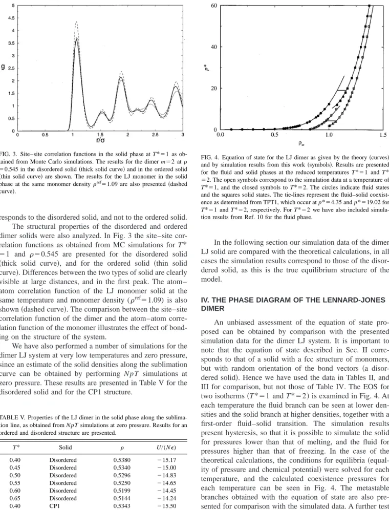
responds to the disordered solid, and not to the ordered solid. The structural properties of the disordered and ordered dimer solids were also analyzed. In Fig. 3 the site–site cor-relation functions as obtained from MC simulations for T* ⫽1 and ⫽0.545 are presented for the disordered solid 共thick solid curve兲, and for the ordered solid 共thin solid curve兲. Differences between the two types of solid are clearly visible at large distances, and in the first peak. The atom– atom correlation function of the LJ monomer solid at the same temperature and monomer density (ref⫽1.09) is also shown共dashed curve兲. The comparison between the site–site correlation function of the dimer and the atom–atom corre-lation function of the monomer illustrates the effect of bond-ing on the structure of the system.
We have also performed a number of simulations for the dimer LJ system at very low temperatures and zero pressure, since an estimate of the solid densities along the sublimation curve can be obtained by performing N pT simulations at zero pressure. These results are presented in Table V for the disordered solid and for the CP1 structure.
In the following section our simulation data of the dimer LJ solid are compared with the theoretical calculations, in all cases the simulation results correspond to those of the disor-dered solid, as this is the true equilibrium structure of the model.
IV. THE PHASE DIAGRAM OF THE LENNARD-JONES DIMER
An unbiased assessment of the equation of state pro-posed can be obtained by comparison with the presented simulation data for the dimer LJ system. It is important to note that the equation of state described in Sec. II corre-sponds to that of a solid with a fcc structure of monomers, but with random orientation of the bond vectors 共a disor-dered solid兲. Hence we have used the data in Tables II, and III for comparison, but not those of Table IV. The EOS for two isotherms共T*⫽1 and T*⫽2兲is examined in Fig. 4. At each temperature the fluid branch can be seen at lower den-sities and the solid branch at higher denden-sities, together with a first-order fluid–solid transition. The simulation results present hysteresis, so that it is possible to simulate the solid for pressures lower than that of melting, and the fluid for pressures higher than that of freezing. In the case of the theoretical calculations, the conditions for equilibria共 equal-ity of pressure and chemical potential兲were solved for each temperature, and the calculated coexistence pressures for each temperature can be seen in Fig. 4. The metastable branches obtained with the equation of state are also pre-sented for comparison with the simulated data. A further test of the theory is provided by an examination of the internal energy. In Fig. 5 the simulation data of the internal energy of the dimer are compared to the theoretical predictions for temperatures T*⫽1 and T*⫽2. The agreement between the FIG. 3. Site–site correlation functions in the solid phase at T*⫽1 as
ob-tained from Monte Carlo simulations. The results for the dimer m⫽2 at ⫽0.545 in the disordered solid共thick solid curve兲and in the ordered solid
共thin solid curve兲are shown. The results for the LJ monomer in the solid phase at the same monomer density ref⫽1.09 are also presented共dashed curve兲.
TABLE V. Properties of the LJ dimer in the solid phase along the sublima-tion line, as obtained from N pT simulasublima-tions at zero pressure. Results for an ordered and disordered structure are presented.
T* Solid U/(N⑀)
0.40 Disordered 0.5380 ⫺15.17
0.45 Disordered 0.5340 ⫺15.00
0.50 Disordered 0.5296 ⫺14.83
0.55 Disordered 0.5250 ⫺14.65
0.60 Disordered 0.5199 ⫺14.45
0.65 Disordered 0.5144 ⫺14.24
0.40 CP1 0.5343 ⫺15.50
0.50 CP1 0.5260 ⫺15.16
0.55 CP1 0.5216 ⫺14.98
0.60 CP1 0.5169 ⫺14.79
0.65 CP1 0.5118 ⫺14.59
FIG. 4. Equation of state for the LJ dimer as given by the theory共curves兲 and by simulation results from this work共symbols兲. Results are presented for the fluid and solid phases at the reduced temperatures T*⫽1 and T* ⫽2. The open symbols correspond to the simulation data at a temperature of
T*⫽1, and the closed symbols to T*⫽2. The circles indicate fluid states and the squares solid states. The tie-lines represent the fluid–solid coexist-ence as determined from TPT1, which occur at p*⫽4.35 and p*⫽19.02 for
simulation data and the calculations is found to be very good over the wide range of densities considered, both for the equation of state data, and for the internal energy data.
In Fig. 6共a兲the global phase diagram for the LJ dimer as obtained from Wertheim’s TPT1 for the fluid and solid phase is presented. The Gibbs ensemble simulation data for the vapor–liquid equilibria of the LJ dimer as reported by Dubey et al.41have been included, together with our simulation re-sults for the zero-pressure densities of the LJ dimer solid at low temperatures. Since the vapor–pressure 共in reduced units兲is very small along the vapor–solid coexistence curve, these simulations provide a good estimate of the solid den-sities along the sublimation curve. As can be seen, the theory describes very accurately the available simulation results of the phase diagram of the LJ dimer. The triple point tempera-ture for the LJ dimer as estimated from the theory presented in this work is Tt*⫽0.653. In the case of the monomer LJ system, the triple point temperature predicted by the theory (Tt*⫽0.687) is in excellent agreement with the estimate of Agrawal and Kofke42 (Tt*⫽0.687). As can be seen, the triple point temperature of the LJ dimer is 5% lower than that of the LJ monomer. Differences in the triple point densities are somewhat larger, as can be seen in Fig. 6共b兲. Following the encouraging results obtained for the dimer system we continue, in the next section, to study the phase behavior of longer chain molecules.
V. GLOBAL PHASE DIAGRAM FOR LJ CHAINS
Using the theory presented in Sec. II, we have also stud-ied the phase behavior of fully-flexible Lennard-Jones chains of lengths m⫽4 and m⫽8. In Fig. 7共a兲 the temperature– density (T*m) projection of the phase diagram is shown,
where, as in the previous section, the reduced density corre-sponds to the reduced monomer density. The phase envelope
corresponding to the monomer m⫽1 and dimer m⫽2
Lennard-Jones systems are included for comparison. As
ex-pected, an increase of the chain length results in a more dramatic variation of the vapor–liquid coexistence than of the solid–liquid and solid–gas phase boundaries. Since the theoretical predictions corresponding to the fluid phases have been discussed in detail elsewhere共see Refs. 13–15兲, in this work we concentrate on the study of the solid–fluid equilib-ria. For each chain length, the liquid–solid transition densi-ties are found to increase with temperature. The increase is more pronounced in the monomer system than for longer chains. The temperature at which solid, liquid, and gas are found in coexistence共the triple point temperature兲is seen to decrease with increasing chain length 关see Fig. 7共b兲 and Table VI for more details兴. Below the triple point tempera-ture, solid–gas coexistence is observed. The binodal curves corresponding to the solid phase associated to the solid–gas phase transition shift toward higher densities for increasing chain length. As in the case of the solid–liquid coexistence curves, the largest change in the solid–gas phase boundaries is observed between the monomer and the dimer.
FIG. 5. Configurational internal energy U/(N⑀) for the LJ dimer as given by the theory共curves兲and by simulation results from this work共symbols兲. Results are presented for the fluid and solid phases at the reduced tempera-tures T*⫽1 and T*⫽2. The rest of the notation is as in Fig. 4. For T* ⫽2 we have also included simulation results from Ref. 10 for the fluid phase.
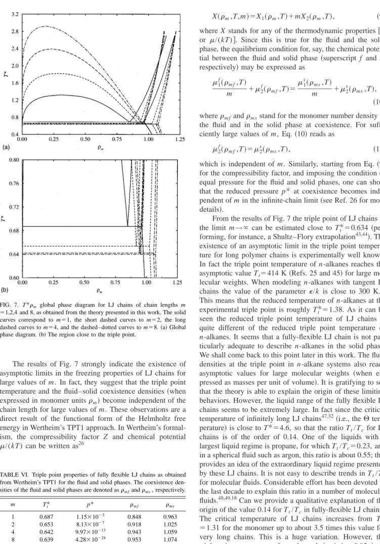
The results of Fig. 7 strongly indicate the existence of asymptotic limits in the freezing properties of LJ chains for large values of m. In fact, they suggest that the triple point temperature and the fluid–solid coexistence densities共when expressed in monomer unitsm) become independent of the chain length for large values of m. These observations are a direct result of the functional form of the Helmholtz free energy in Wertheim’s TPT1 approach. In Wertheim’s formal-ism, the compressibility factor Z and chemical potential /(kT) can be written as26
X共m,T,m兲⫽X1共m,T兲⫹mX2共m,T兲, 共9兲
where X stands for any of the thermodynamic properties关Z or /(kT)兴. Since this is true for the fluid and the solid phase, the equilibrium condition for, say, the chemical poten-tial between the fluid and solid phase 共superscript f and s, respectively兲may be expressed as
1 f共
m f,T兲
m ⫹2
f共
m f,T兲⫽
1 s共
ms,T兲
m ⫹2
s共
ms,T兲,
共10兲 wherem fandmsstand for the monomer number density in
the fluid and in the solid phase at coexistence. For suffi-ciently large values of m, Eq. 共10兲reads as
2 f共
m f,T兲⫽2 s共
ms,T兲, 共11兲
which is independent of m. Similarly, starting from Eq. 共9兲 for the compressibility factor, and imposing the condition of equal pressure for the fluid and solid phases, one can show that the reduced pressure p* at coexistence becomes inde-pendent of m in the infinite-chain limit共see Ref. 26 for more details兲.
From the results of Fig. 7 the triple point of LJ chains in the limit m→⬁ can be estimated close to Tt*⫽0.634 共 per-forming, for instance, a Shultz–Flory extrapolation43,44兲. The existence of an asymptotic limit in the triple point tempera-ture for long polymer chains is experimentally well known. In fact the triple point temperature of n-alkanes reaches the asymptotic value Tt⫽414 K共Refs. 25 and 45兲for large
mo-lecular weights. When modeling n-alkanes with tangent LJ chains the value of the parameter ⑀/k is close to 300 K.46 This means that the reduced temperature of n-alkanes at the experimental triple point is roughly Tt*⫽1.38. As it can be seen the reduced triple point temperature of LJ chains is quite different of the reduced triple point temperature of n-alkanes. It seems that a fully-flexible LJ chain is not par-ticularly adequate to describe n-alkanes in the solid phase. We shall come back to this point later in this work. The fluid densities at the triple point in n-alkane systems also reach asymptotic values for large molecular weights 共when ex-pressed as masses per unit of volume兲. It is gratifying to see that the theory is able to explain the origin of these limiting behaviors. However, the liquid range of the fully flexible LJ chains seems to be extremely large. In fact since the critical temperature of infinitely long LJ chains47,32共i.e., the⌰ tem-perature兲 is close to T*⫽4.6, so that the ratio Tt/Tc for LJ chains is of the order of 0.14. One of the liquids with a largest liquid regime is propane, for which Tt/Tc⫽0.23, and in a spherical fluid such as argon, this ratio is about 0.55; this provides an idea of the extraordinary liquid regime presented by these LJ chains. It is not easy to describe trends in Tt/Tc
for molecular fluids. Considerable effort has been devoted in the last decade to explain this ratio in a number of molecular fluids.48,49,18Can we provide a qualitative explanation of the origin of the value 0.14 for Tt/Tcin fully-flexible LJ chains?
The critical temperature of LJ chains increases from T* ⫽1.31 for the monomer up to about 3.5 times this value for very long chains. This is a huge variation. However, the triple point temperature of very long chains is just 0.93 times FIG. 7. T*m global phase diagram for LJ chains of chain lengths m
⫽1,2,4 and 8, as obtained from the theory presented in this work. The solid curves correspond to m⫽1, the short dashed curves to m⫽2, the long dashed curves to m⫽4, and the dashed–dotted curves to m⫽8.共a兲Global phase diagram.共b兲The region close to the triple point.
TABLE VI. Triple point properties of fully flexible LJ chains as obtained from Wertheim’s TPT1 for the fluid and solid phases. The coexistence den-sities of the fluid and solid phases are denoted asm fandms, respectively.
m Tt* p* m f ms
1 0.687 1.15⫻10⫺3 0.848 0.963
2 0.653 8.13⫻10⫺7 0.918 1.025
4 0.642 9.97⫻10⫺13 0.943 1.059
that of the LJ monomer. One can understand easily the enor-mous increases of the critical temperature of LJ chains with respect to the monomer. How to understand the almost con-stant value for the triple point temperature? As can be seen in Fig. 7, at low temperatures the increase of the orthobaric density from m⫽1 to m⫽2 is almost identical to the in-crease in the density at freezing from m⫽1 to m⫽2, so that the triple point temperature remains practically unaffected. Of course this is not exact, but it provides a simple view as to why the triple point temperature is approximately con-stant.
It is useful to examine also the p*T* projection of the phase diagram as obtained with the theoretical approach共see Fig. 8兲. In Fig. 8共a兲the vapor–pressure curve, solid–liquid transition line, and solid–gas transition line corresponding to freely-jointed Lennard-Jones chains of up to eight monomers (m⫽8) are presented. The coexistence lines of the Lennard-Jones monomer system are included for comparison. It is more interesting to analyze the high-pressure region of the p*T* projection of the phase diagram 关Fig. 8共b兲兴. The liquid–vapor and solid–gas coexistence curves cannot be seen in this plot since these boundaries occur at very low
pressures compared to the range at which solid–liquid tran-sition continues. As can be seen, at low temperatures the fluid–solid transition pressures increase with increasing m, however, at high temperatures this trend is inverted, and the solid–liquid transition pressures decrease for increasing chain lengths. The slope in the p*T*is related to the melting enthalpy and to the volume change through the Clapeyron equation.50
VI. CONCLUSIONS
In this work Wertheim’s TPT1 theory has been extended to study the solid phase of LJ chains. The theory requires a knowledge of the free energy and of the contact value of the radial distribution function of the reference LJ monomer. Johnson et al.9,10 have given expressions for both of these properties in the fluid phase, and van der Hoef34has recently proposed an expression for the free energy of the solid phase. In order to determine gref() in the solid phase we have performed computer simulations and fitted the numerical re-sults to an empirical expression of the same form as that proposed by Johnson et al.10 The theory has been tested by comparing simulation and theoretical results for the LJ dimer. For this purpose computer simulations were per-formed for the disordered solid structure of the LJ dimer. It has been shown that the theory describes very accurately the EOS and internal energy of the LJ dimer solid. Furthermore, the densities of the solid along the sublimation curve are also found to be in excellent agreement with simulation data. Our estimate of the triple point temperature for the LJ dimer is Tt*⫽0.653. Using Wertheim’s TPT1 for the fluid and for the solid phase we have calculated the vapor–liquid, liquid– solid, and solid–vapor coexistence lines as well as the global phase diagram of LJ chains.
Studying longer chain molecules, it has been shown that the calculated triple point temperature of LJ chains tends to an asymptotic finite value of Tt*⫽0.634, which means that the chains present an enormous liquid range 共i.e., Tt/Tc
⫽0.14兲. The calculated coexistence densities 共when ex-pressed in monomers per unit of volume m兲 also tend to
asymptotic values for large values of m. Although the model used in this work is a crude one, it is able to capture some of the features presented in the phase diagram of real flexible molecules. In polyethylene the triple point temperature reaches a finite value and the fluid–solid coexistence densi-ties become very similar for large chain lengths 共when the densities are expressed in units of mass per volume兲.
It should be noted, however, that fully flexible models may not be particularly realistic when describing solid phases of real substances. The extreme flexibility of the LJ chain allows the existence of a singular solid with ordering of atoms but disorder of bonds. It must be mentioned that such a solid cannot be constructed using real polymers; over-lap between contiguous monomers, whose distance is less than the sum of their van der Waals radii, and the existence of bond angles and torsional potentials make such a high-density disordered solid an impossibility. When these geo-metrical constraints are included in the model, the only way of obtaining a highly-packed solid is to generate an ordered FIG. 8. p*T*representation of the global phase diagram for LJ chains with
solid, in which the bonds are also ordered. Certainly, real chains are not formed by fully flexible tangent LJ segments; this is reflected in the fact that the Tt/Tc ratio for
polyethylene51is close to 0.40共with some recent estimates of Tc of polyethylene
52
this ratio will be somewhat smaller, namely, 0.34兲in contrast to the value Tt/Tc⫽0.14 obtained
in this work using fully flexible LJ chains. Obviously, chemi-cal and geometrichemi-cal details of the molecule matter when dealing with the description of solid phases. The fully flex-ible LJ model does not seem to be the most appropriate model to describe the solid structure of n-alkanes. This was not our goal here, but rather to determine the phase diagram of LJ chains in a full theoretical manner, and to show that a very simple model can be useful in explaining some of the trends共not the actual values兲in a number of properties of the phase diagram of real polymers.
Concerning the issue of whether the theory presented here could be useful, in an engineering sense, to describe the global phase behavior 共vapor–liquid, vapor–solid, liquid– solid equilibrium兲of real chains, we believe that the answer is, in principle, no. One cannot reproduce the value Tt/Tc
⫽0.4 of polyethylene51 with a model that yields Tt/Tc
⫽0.14. The freely jointed LJ chain is not a good model for an n-alkane after all. A look at the important differences in the freezing properties of freely jointed hard sphere chains and hard models of n-alkanes with a realistic description of the molecular shape already suggests this.19,20 This paper provides further evidence. Although we can describe n-alkanes in the fluid phase using a freely jointed LJ chain model, after fitting all the parameters to experimental prop-erties, the model will never be able to describe correctly the
global phase diagram of an n-alkane 共including solid
phases兲. If a model is required to describe the complete phase diagram of n-alkanes, models such as the Ryckaert and Bellemans,53and their modern variations,54 –56which include the geometrical details of the molecule, might be more prom-ising. Maybe a less ambitious approach is possible if one allows a different set of potential parameters for the fluid and the solid phase, or if a set of potential parameters is used solely to describe the solid phase. This does not seem to be justified from a molecular point of view 共molecular param-eters of the potential should be the same in the fluid and solid phase兲but could be of interest for practical applications.
ACKNOWLEDGMENTS
Financial support is due to Project No. BFM-2001-1420-C02-01 and BFM-2001-1420-C02-02 of the Spanish DGI-CYT 共Direccio´n General de Investigacio´n Cientı´fica y Te´c-nica兲. F.J.B. would like to acknowledge the Universidad de Huelva and Junta de Andalucı´a for additional financial sup-port. A.G. would like to thank the Engineering and Physical Sciences Research Council for the award of an Advanced Research Fellowship.
1M. S. Wertheim, J. Stat. Phys. 35, 19共1984兲. 2M. S. Wertheim, J. Stat. Phys. 35, 35共1984兲. 3
M. S. Wertheim, J. Stat. Phys. 42, 459共1986兲.
4M. S. Wertheim, J. Stat. Phys. 42, 477共1986兲. 5M. S. Wertheim, J. Chem. Phys. 85, 2929共1986兲.
6M. S. Wertheim, J. Chem. Phys. 87, 7323共1987兲.
7W. G. Chapman, G. Jackson, and K. E. Gubbins, Mol. Phys. 65, 1057
共1988兲.
8W. G. Chapman, J. Chem. Phys. 93, 4299共1990兲.
9J. K. Johnson, J. A. Zollweg, and K. E. Gubbins, Mol. Phys. 78, 591
共1993兲.
10J. K. Johnson, E. A. Mu¨ller, and K. E. Gubbins, J. Phys. Chem. 98, 6413
共1994兲.
11A. Gil-Villegas, A. Galindo, P. J. Whitehead, S. J. Mills, G. Jackson, and
A. N. Burgess, J. Chem. Phys. 106, 4168共1997兲.
12
L. A. Davies, A. Gil-Villegas, and G. Jackson, J. Chem. Phys. 111, 8659
共1999兲.
13F. A. Escobedo and J. J. de Pablo, Mol. Phys. 87, 347共1996兲. 14
F. J. Blas and L. F. Vega, Mol. Phys. 92, 1共1997兲.
15F. J. Blas and L. F. Vega, J. Chem. Phys. 115, 4355共2001兲.
16L. G. MacDowell, M. Mu¨ller, C. Vega, and K. Binder, J. Chem. Phys. 113,
419共2000兲.
17C. T. Lin and G. Stell, J. Chem. Phys. 114, 6969共2001兲. 18
P. A. Monson and D. A. Kofke, Adv. Chem. Phys. 115, 113共2000兲.
19A. P. Malanoski and P. A. Monson, J. Chem. Phys. 107, 6899共1997兲. 20A. P. Malanoski and P. A. Monson, J. Chem. Phys. 110, 664共1999兲. 21
J. M. Polson and D. Frenkel, J. Chem. Phys. 109, 318共1998兲.
22J. M. Polson and D. Frenkel, J. Chem. Phys. 111, 1501共1999兲. 23R. P. Sear and G. Jackson, J. Chem. Phys. 102, 939共1995兲. 24
A. P. Malanoski, C. Vega, and P. A. Monson, Mol. Phys. 98, 363共2000兲.
25R. C. Reid, J. M. Prausnitz, and B. E. Poling, The Properties of Gases and
Liquids, 4th ed.共McGraw–Hill, New York, 1987兲.
26C. Vega and L. G. MacDowell, J. Chem. Phys. 114, 10411共2001兲. 27C. McBride and C. Vega, J. Chem. Phys. 116, 1757共2002兲. 28
K. W. Wojciechowski, A. C. Branka, and D. Frenkel, Physica A 196, 519
共1993兲.
29K. W. Wojciechowski, D. Frenkel, and A. C. Branka, Phys. Rev. Lett. 66,
3168共1991兲.
30Y. Zhou and G. Stell, J. Chem. Phys. 96, 1507共1992兲.
31W. R. Smith, I. Nezbeda, M. Strnad, B. Triska, S. Labik, and A.
Malijevsky, J. Chem. Phys. 109, 1052共1998兲.
32C. Vega and L. G. MacDowell, Mol. Phys. 98, 1295共2000兲. 33
D. A. McQuarrie, Statistical Mechanics 共Harper and Row, New York, 1976兲.
34M. A. van der Hoef, J. Chem. Phys. 113, 8142共2000兲. 35
M. P. Allen and D. J. Tildesley, Computer Simulation of Liquids, 2nd ed.
共Clarendon, Oxford, 1987兲.
36A. Brooke, D. Kendrick, A. Meeraus, and R. Raman, GAMS, A User’s
Guide, GAMS Development Corporation.
37R. Bowles and R. J. Speedy, Mol. Phys. 87, 1349共1996兲.
38C. Vega, E. P. A. Paras, and P. A. Monson, J. Chem. Phys. 96, 9060
共1992兲.
39M. Parrinello and A. Rahman, Phys. Rev. Lett. 45, 1196共1980兲. 40
S. Yashonath and C. N. R. Rao, Mol. Phys. 54, 245共1985兲.
41G. S. Dubey, S. O’Shea, and P. A. Monson, Mol. Phys. 80, 997共1993兲. 42R. Agrawal and D. A. Kofke, Mol. Phys. 85, 43共1995兲.
43
A. R. Shultz and P. J. Flory, J. Am. Chem. Soc. 74, 4760共1952兲.
44P. J. Flory, Principles of Polymer Chemistry共Cornell University Press,
Ithaca, 1954兲.
45
M. G. Broadhurst, J. Res. Natl. Bur. Stand., Sect. A 66A, 241共1962兲.
46J. C. Pamies and L. F. Vega, Ind. Eng. Chem. Res. 40, 2532共2001兲. 47
Y. J. Sheng, A. Z. Panagiotopoulos, and S. K. Kumar, Macromolecules 27, 400共1994兲.
48E. P. A. Paras, C. Vega, and P. A. Monson, Mol. Phys. 79, 1063共1993兲. 49
C. Vega, B. Garzon, S. Lago, and P. A. Monson, J. Mol. Liq. 76, 157
共1998兲.
50D. A. McQuarrie and J. D. Simon, Physical Chemistry: A Molecular
Ap-proach共University Science Books, Sausalito, 1997兲.
51D. L. Morgan and R. Kobayashi, Fluid Phase Equilib. 63, 317共1991兲. 52E. D. Nikitin, High Temp. 36, 305共1998兲.
53J. P. Ryckaert and A. Bellemans, Faraday Discuss. Chem. Soc. 66, 95
共1978兲.
54
A. Lopez Rodriguez, C. Vega, J. J. Freire, and S. Lago, Mol. Phys. 80, 1565共1993兲.
55B. Smit, S. Karaborni, and J. I. Siepmann, J. Chem. Phys. 102, 2126
共1995兲; 109, 352共E兲 共1998兲.
56A. Lopez Rodriguez, C. Vega, and J. J. Freire, J. Chem. Phys. 111, 438