The phase diagram of the two center Lennard-Jones model as obtained
from computer simulation and Wertheim’s thermodynamic
perturbation theory
C. Vegaa) and C. McBride
Departamento de Quı´mica Fı´sica, Facultad de Ciencias Quı´micas, Universidad Complutense de Madrid, Ciudad Universitaria 28040 Madrid, Spain
E. de Miguel and F. J. Blas
Departamento de Fı´sica Aplicada, Facultad de Ciencias Experimentales, Universidad de Huelva, 21071, Huelva, Spain
A. Galindo
Department of Chemical Engineering and Chemical Technology, Imperial College, London, South Kensington Campus, London SW7 2AZ United Kingdom
共Received 24 January 2003; accepted 14 March 2003兲
The global phase diagram 共i.e., vapor–liquid and fluid–solid equilibrium兲 of two-center Lennard-Jones 共2CLJ兲 model molecules of bond length L⫽ has been determined by computer simulation. The vapor–liquid equilibrium conditions are obtained using the Gibbs ensemble Monte Carlo method and by performing isobaric-isothermal NPT calculations at zero pressure. In the case of the solid phase, two close-packed solid structures are considered: In the first structure, the molecules are located in layers and all molecular axes point in the same direction; and in the second structure, the atoms form a close-packed arrangement but the molecular axes of the diatomic molecules have random orientations. It is shown that at the vapor–liquid–solid triple-point temperature, the orientationally disordered solid is the stable structure for the solid phase of this model. The vapor–liquid-disordered solid triple-point temperature of the 2CLJ model, with bond length L⫽, is located at T*⫽0.650(4). This is very close to the triple-point temperature of the Lennard-Jones monomer system (T*⫽0.687). At very low temperatures, the ordered solid is the stable phase. The vapor-ordered solid-disordered solid triple point is situated at T*⫽0.282. The simulation data are compared to Wertheim’s first-order thermodynamic perturbation theory共TPT1兲 for the fluid and solid phases. It is found that Wertheim’s TPT1 not only provides an accurate description of the equation of state in both the fluid and solid phases, but also provides accurate values of the free energies. The prediction of Wertheim’s TPT1 for the global phase diagram of the 2CLJ model shows excellent agreement with the simulation results, illustrating the possibility of using Wertheim’s perturbation theory to determine not only the vapor–liquid equilibria but also the global phase diagram of simple chain model molecules. © 2003 American Institute of Physics.
关DOI: 10.1063/1.1572811兴
I. INTRODUCTION
Since the initial computer simulations in the 1950’s, a considerable amount of work has been devoted to the deter-mination of the phase diagrams of model molecular systems. The calculation, by means of computer simulation, of the phase diagrams of the hard-sphere1,2 and Lennard-Jones monomer systems3have played an important role in improv-ing our understandimprov-ing of the states of matter. In the last twenty years, the phase diagrams of a number of model sys-tems 共including solid and liquid-crystalline phases兲 have been obtained by using computer simulation. For example, studies have been carried out for hard ellipsoids,4 hard spherocylinders,5hard cut spheres,6hard dumbbells,7–9 qua-drupolar hard dumbbells,10 fully flexible hard chains,11,12
hard charged spheres,13–15 Gay–Berne molecules,16,17 and simple point charge model water molecules.18
The calculation of the complete phase diagram of a pro-posed model system can now be carried out within a reason-able amount of time due to the increased speed of modern computers. However, brute force computational power is not the only key to the success of simulation studies; much credit is due to the development of simulation techniques for the determination of phase equilibria. These techniques are the Gibbs ensemble Monte Carlo19 and the NPT⫹test particle methods,20which are very useful in determining the vapor– liquid equilibria, the Gibbs–Duhem integration method,21,22 which becomes an invaluable tool when determining fluid– solid equilibria, the Rahman–Parrinello technique, essential in the study of solid phases,23,24and Einstein-crystal calcu-lations, which provide the free energies of solid phases.25A general approach to the determination of global phase dia-grams by computer simulation would entail:
a兲Electronic mail: [email protected]
10696
共a兲 Obtaining the vapor–liquid equilibria using the Gibbs ensemble Monte Carlo technique 共or the NPT⫹test particle method兲, and determining the orthobaric den-sities at low pressures by carrying out NPT simulations at zero pressure.
共b兲 Determining the equation of state 共EOS兲 of the solid for one isotherm using the Rahman–Parrinello tech-nique 共or one of its Monte Carlo counterparts兲, and performing free-energy calculations in the equilibrium unit cell using Einstein-crystal calculations.
共c兲 Performing a Gibbs–Duhem integration to obtain the complete fluid–solid equilibrium curve.
These are the steps that have been followed in the determi-nation of the global phase diagram of model two-center Lennard-Jones共2CLJ兲molecules studied in this work.
Following the success of the Lennard-Jones共LJ兲 inter-molecular potential as a model for atomic fluids, one of the simplest molecular models that can be proposed is the 2CLJ. This model consists of two LJ centers with potential param-eters⑀andseparated from one another by a reduced bond length of L*⫽L/. The vapor–liquid equilibria of 2CLJ model molecules with different values of L*has been stud-ied by a number of authors,26 –30and has been the subject of interest in a large number of theoretical studies.31–35 Some-what surprisingly, the fluid–solid equilibria has not been considered in detail, the only exception being the work of Lisal and Vacek36 who have determined the global phase diagram 共vapor–liquid–solid兲 for a 2CLJ system with L*⫽0.67 by molecular-dynamics computer simulations and using the Gibbs–Duhem integration method.
In terms of theoretical developments in the field of per-turbation theory and equations of state of complex fluids, in the 1980’s Wertheim37– 40 presented a series of seminal pa-pers developing a theory for associating fluids. It has since been shown that when the association strength becomes in-finitely strong, chains can be formed from a fluid of associ-ating monomers,41,42thus, an EOS for a chain composed of freely jointed tangent monomers can be derived solely using the thermodynamic information of the monomer reference fluid. In the simplest implementation of the theory, known as first-order thermodynamic perturbation theory 共TPT1兲, the only information required to build an approximate EOS for the chain fluid is the EOS and the pair correlation function of the monomer fluid at contact. Although Wertheim’s formal-ism was originally aimed at the study of hard chains, it was soon realized that it could also be applied to LJ chains.43– 47 Recently, we have explored the possibility of furthering the usefulness of Wertheim’s TPT1 by applying it to the solid phase. Vega and MacDowell48 have shown that Wertheim’s TPT1 can be employed in the treatment of the solid phase for freely jointed hard-sphere chain molecules, obtaining excel-lent agreement with the simulation results of Malanoski and Monson.11 This work has been extended by Blas et al.49 to deal with fully flexible hard-chain molecules with segment– segment attractive interactions treated at the mean-field level of van der Waals. Similar results have also been obtained in two dimensions.50 Encouraged by these findings, we have extended Wertheim’s TPT1 to model the solid phase of LJ
chains,51 and have been able to show that the approach pro-vides a good description of the EOS and good results for the internal energy of the solid phase of LJ tangent dimers共2CLJ with L*⫽1). It is important to note that Wertheim’s TPT1 can only be used to describe chains formed by ‘‘tangent’’ spheres共i.e., those with reduced bond lengths L*⫽1). Since Wertheim’s TPT1 can provide an accurate description of the EOS of the 2CLJ model with L*⫽1 in the fluid and solid phases, it is natural to wonder whether it could be used to describe the global phase diagram of the 2CLJ model. It is important to mention at this stage that an accurate EOS for the solid phase does not necessarily guarantee the correct prediction of the fluid–solid equilibria, as the theoretical ap-proach must also provide good estimates for the free energies in the solid phase. In this work, we determine the phase diagram of the 2CLJ model 共with L*⫽1) using computer simulations, and we compare the phase diagram obtained in this way with that obtained using Wertheim’s TPT1.
The study of the solid phases of 2CLJ model molecules implies that a number of structures should be considered. While a system of LJ monomers freezes into a face-centered-cubic 共fcc兲 close-packed arrangement, in the case of 2CLJ molecules with L*⫽1, it is possible to construct, based on the closed-packed configuration of the LJ monomer solid, a number of distinct solid structures. Vega, Paras, and Monson8 have presented several structures of this type for hard diatomic 共hard dumbbell兲 molecules; each of the ar-rangements are possible configurations for 2CLJ molecules. In these structures, the molecules are located in layers, and the molecular axes of all the molecules in a layer point in the same direction. In the particular case of the so-called closed-packed 1 共CP1兲structure, the molecular axes of each of the molecules in each of the layers point in the same direction. In the present work, the CP1 configuration is considered as one of the possible solid structures of the 2CLJ tangent model. This CP1 solid structure will be denoted as the or-dered solid. It was found in Ref. 8 that the differences be-tween the free energies of different ordered solid structures were small, indicating that the CP1 is a good representative of these ordered structures. However, it is unlikely that or-dered structures correspond to the stable solid phase for the 2CLJ tangent model. Wojciechowski, and co-workers52,53 were the first to suggest that for L*⫽1, it is possible to build a solid structure where the atoms follow an fcc close-packed arrangement, but where the bonds are randomly located within the solid, with no long-range orientational order be-tween the bond vectors. We also consider this structure in this work and denote it the disordered solid. In fact, Wojciechowski et al.52,53 have shown that the stable solid structure of tangent hard-disk dimers in two dimensions is formed by a close-packed arrangement of atoms with a dis-ordered arrangement of bonds. The same idea holds true for hard chains in three dimensions,11and one may expect that the same would occur for a three-dimensional 2CLJ tangent dimer. In this work, it will be shown that the disordered solid is the stable solid structure for most thermodynamic condi-tions 共with the exception of very low temperatures兲.
is described, in Sec. III, we provide details of the computer simulations performed in this work, in Sec. IV, the results are presented, and in Sec. V, conclusions are discussed.
II. BRIEF DESCRIPTION OF WERTHEIM’S PERTURBATION THEORY
It is now well known that Wertheim’s TPT1 can be used to describe the properties of LJ chains in the fluid phase.54 This was first suggested by Chapman,43 and later confirmed by Johnson et al.45The possibility of extending Wertheim’s TPT1 to treat solid phases has only recently been explored.48,50,51 It has been shown that an accurate descrip-tion of the EOS and internal energies of the 2CLJ tangent model in the solid phase can be obtained following the ideas of the TPT1 theory of Wertheim. Details of the extension of Wertheim’s TPT1 to model solid phases of LJ chains have been given elsewhere;51here, we provide only an overview of the main features of the approach.
Let us assume that we have a certain number Nref of spherical monomer particles within a volume V at tempera-ture T. These spherical particles interact through a spherical pair potential uref(r); in this work, the pair potential uref(r)
is the LJ potential with parameters and⑀. We denote this fluid as the reference fluid, and label its properties with the superscript ref. Let us also assume that in another container of volume V at temperature T, we have N⫽Nref/m fully flexible chains of m monomers each. By fully flexible chains, we mean chains of m monomers with fixed bond lengths between monomers L⫽, and no other constraints 共i.e., there is no restriction of either the bonding angles or of the torsional angles兲. Each monomer of a given chain interacts with all the other monomers in the system, either in the same molecule, or in other molecules, with the only exception of the monomer/s to which it is bonded, interacting via the pair potential uref(r). The chain system described so far will be denoted as the chain fluid. It follows from Wertheim’s TPT1 that the free energy A of the chain model system can be written as
A
NkBT
⫽ln共3兲⫺1⫹mAresidual ref
NrefkBT
⫺共m⫺1兲ln yref共兲,
共1兲
where kB is Boltzmann’s constant, and⫽N/V the molecu-lar number density. In Eq. 共1兲, we have set the de Broglie thermal wavelength to. This expression indicates that the free energy of the chain may be obtained from a knowledge of the residual free energy of the reference fluid Aresidualref and the background pair correlation function yref() of the
refer-ence fluid at the bonding distance .55,56 As y (r)
⫽exp关u(r)/kBT兴g(r), and since in the case of the LJ potential model the pair potential is zero at r⫽, for this particular choice of bond length, y ()⫽g(). Replacing y () by g() in Eq.共1兲, and differentiating the free energy with re-spect to density, the EOS is given by
Z⫽mZref⫺共m⫺1兲
冉
1⫹ref ln gref共兲
ref
冊
, 共2兲where we have defined the compressibility factor of the ref-erence monomer system as Zref⫽Pref/(refkBT), with P be-ing the pressure. The correspondbe-ing residual part of the in-ternal energy U is given by
U
NkBT⫽
m U
ref
NrefkBT⫹共
m⫺1兲T
冉
ln gref共兲
T
冊
. 共3兲We denote Eqs.共1兲–共3兲as Wertheim’s TPT1 theory. It is useful to note here that the arguments used to derive Eqs.共1兲–共3兲make no special mention of the actual nature of the phase considered,48,57,58thus, this approach can be used to describe both fluid and solid phases. In such a case, all that is needed in order to obtain a unified theory for the global phase equilibria of chain molecules is the residual free energy, compressibility factor, and pair correlation function of the monomer system both in the fluid and solid phases. Johnson et al.44,45have provided values of the free energy and structural properties 关i.e., gref()] for the monomer LJ fluid. In this work, we follow their implementation of the TPT1 of Wertheim to model the fluid phases of 2CLJ mol-ecules.
Van der Hoef59 has recently presented an analytical ex-pression for the free energy of the LJ monomer solid ob-tained by fitting the most recent simulation results for the solid phase of this model to a simple functional expression. We shall use his expression in this work. Values of gref() for the LJ monomer solid, which are also required in the TPT1 approach, were obtained by computer simulation in a previous work51for a number of temperatures and densities. The simulations results for gref() were fitted to an empirical expression of the same polynomial form than that proposed by Johnson et al.45for the fluid phase; the coefficients of the polynomial can be found in Ref. 51.
III. SIMULATION DETAILS
In this work, we consider diatomic LJ model molecules formed by two identical LJ sites 共monomers兲 with a bond distance L⫽, whereis the diameter of the LJ monomer
共i.e., the monomers are tangential兲. We shall refer to the model molecules as 2CLJ tangent. The pair interaction be-tween a pair of molecules is given by
u共1,2兲⫽
兺
i⫽1i⫽2
兺
j⫽1j⫽2
4⑀
冋冉
ri j冊
12
⫺
冉
ri j
冊
6
册
, 共4兲where ri j is the distance between site 共monomer兲 i of mol-ecule 1 and site j of molmol-ecule 2. In order to determine the global phase diagram of the 2CLJ tangent molecules, we have used various simulation techniques. Before describing the details of each technique, it is useful to note that in all the simulations performed, the site–site LJ pair potential was truncated at rc⫽2.5, and long-range corrections were added to all the computed thermodynamic properties 共 inter-nal energy, pressure, and chemical potential兲 by assuming that the site–site pair correlation function is equal to unity beyond the cutoff.60 A cycle is defined as a trial move per particle, and a trial volume change. In the case of the Gibbs ensemble simulations, a cycle also includes Nexattempts to
we use reduced units, so that T*⫽T/(⑀/kB), *⫽3 ⫽(N/V)3, P*⫽P/(⑀/3), and U*⫽U/(N⑀).
A. Vapor–liquid equilibria
The vapor–liquid equilibria of the 2CLJ model has al-ready been considered by a number of authors. Using Gibbs ensemble simulations, Dubey et al.26 have obtained the vapor–liquid equilibria of the 2CLJ model system for several bond lengths, including L*⫽1. More recently, Stoll et al.28 have studied the vapor–liquid transitions for this model us-ing the NPT⫹test particle method. In the latter work, special emphasis was placed on the accurate determination of the critical properties of the system; however, in order to com-pare this with our theoretical calculations, which incorporate the description of the solid phase as well as the fluid phases, we also have an interest in locating the triple point of the 2CLJ model. In this way, computer simulation data of the vapor–liquid equilibria at lower temperatures than reported previously is needed.
We have obtained the vapor–liquid properties of the 2CLJ model fluid with L*⫽1 using the standard Gibbs en-semble Monte Carlo simulation technique. At each tempera-ture T*, an initial configuration is generated by first equili-brating two subsystems 共each containing 500 molecules兲 at the given T*, and with initial vapor and liquid densities close to the expected coexistence values. Constant-volume NVT Monte Carlo simulations are carried out in this equili-bration stage, which consisted of approximately 10 000– 20 000 cycles. The resulting configurations are subsequently used as starting configurations for the Gibbs ensemble run, which consisted of 50 000 equilibration cycles and 50 000 cycles for collecting averages. The coexistence densities, in-ternal energies, pressures, and chemical potentials for each of the temperatures considered are presented in Table I.
At low temperatures, the probability of transferring par-ticles between the two subsystems becomes extremely low
共of the order of 1.9⫻10⫺5 at T*⫽1.0) and, therefore, the Gibbs ensemble technique was found impracticable for tem-peratures T*⬍1.0. As an共approximate兲alternative, we per-formed a series of constant-pressure NPT Monte Carlo simu-lations of the liquid phase at P*⫽0 for temperatures in the range T*⭐1.0. Given that the coexistence pressure at T* ⫽1.0 is P*⫽0.000 59(3), this procedure is expected to yield reliable estimates of the liquid densities at coexistence. Obviously, the estimates improve as T* decreases. The cor-responding results are included in Table II. It is important to note that even in the most unfavorable case (T*⫽1.0), the resulting liquid density obtained with these NPT simulations
关ᐉ*⫽0.4058(14)兴 compares well with the value ᐉ* ⫽0.4061(12) obtained using the Gibbs ensemble technique. As well as determining the location of the triple point, it TABLE I. Vapor–liquid coexistence properties for the 2CLJ model with L*⫽1 as obtained from Gibbs
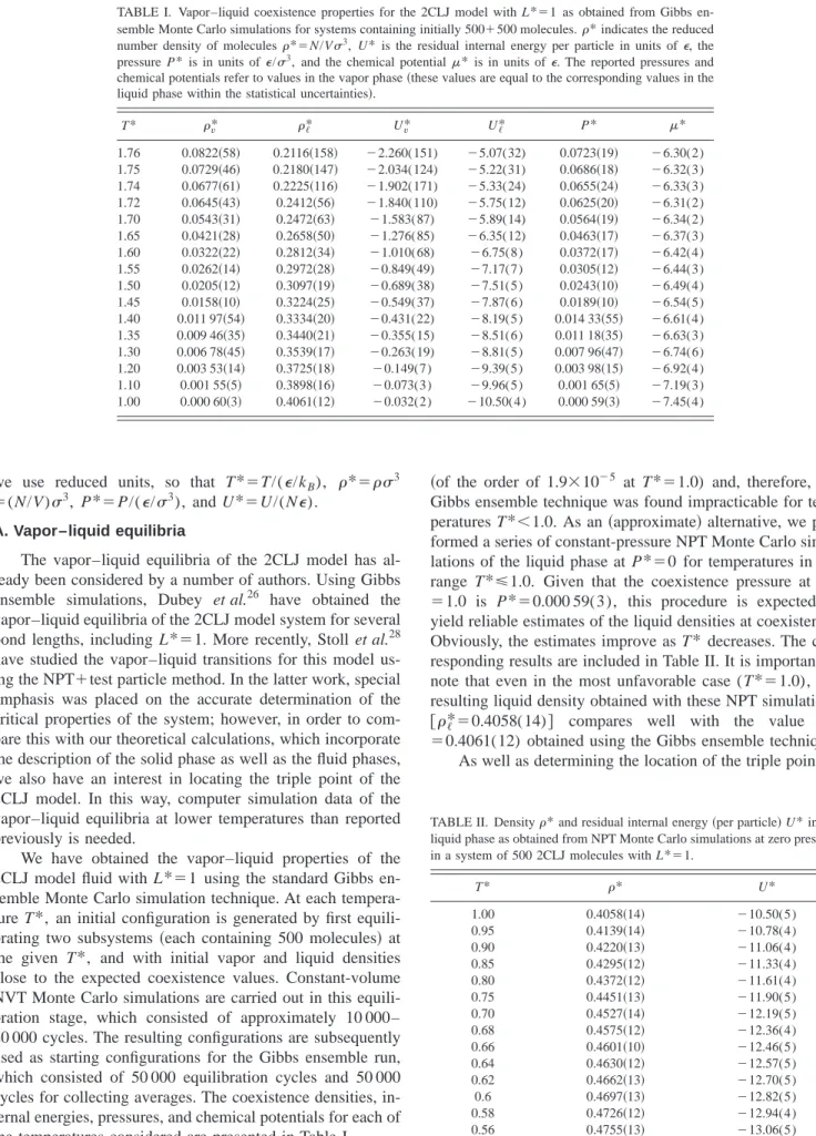
en-semble Monte Carlo simulations for systems containing initially 500⫹500 molecules.*indicates the reduced number density of molecules*⫽N/V3, U*is the residual internal energy per particle in units of⑀, the
pressure P*is in units of⑀/3, and the chemical potential* is in units of⑀. The reported pressures and
chemical potentials refer to values in the vapor phase共these values are equal to the corresponding values in the liquid phase within the statistical uncertainties兲.
T* v* ᐉ* Uv* Uᐉ* P* *
1.76 0.0822共58兲 0.2116共158兲 ⫺2.260(151) ⫺5.07(32) 0.0723共19兲 ⫺6.30(2) 1.75 0.0729共46兲 0.2180共147兲 ⫺2.034(124) ⫺5.22(31) 0.0686共18兲 ⫺6.32(3) 1.74 0.0677共61兲 0.2225共116兲 ⫺1.902(171) ⫺5.33(24) 0.0655共24兲 ⫺6.33(3) 1.72 0.0645共43兲 0.2412共56兲 ⫺1.840(110) ⫺5.75(12) 0.0625共20兲 ⫺6.31(2) 1.70 0.0543共31兲 0.2472共63兲 ⫺1.583(87) ⫺5.89(14) 0.0564共19兲 ⫺6.34(2) 1.65 0.0421共28兲 0.2658共50兲 ⫺1.276(85) ⫺6.35(12) 0.0463共17兲 ⫺6.37(3) 1.60 0.0322共22兲 0.2812共34兲 ⫺1.010(68) ⫺6.75(8) 0.0372共17兲 ⫺6.42(4) 1.55 0.0262共14兲 0.2972共28兲 ⫺0.849(49) ⫺7.17(7) 0.0305共12兲 ⫺6.44(3) 1.50 0.0205共12兲 0.3097共19兲 ⫺0.689(38) ⫺7.51(5) 0.0243共10兲 ⫺6.49(4) 1.45 0.0158共10兲 0.3224共25兲 ⫺0.549(37) ⫺7.87(6) 0.0189共10兲 ⫺6.54(5) 1.40 0.011 97共54兲 0.3334共20兲 ⫺0.431(22) ⫺8.19(5) 0.014 33共55兲 ⫺6.61(4) 1.35 0.009 46共35兲 0.3440共21兲 ⫺0.355(15) ⫺8.51(6) 0.011 18共35兲 ⫺6.63(3) 1.30 0.006 78共45兲 0.3539共17兲 ⫺0.263(19) ⫺8.81(5) 0.007 96共47兲 ⫺6.74(6) 1.20 0.003 53共14兲 0.3725共18兲 ⫺0.149(7) ⫺9.39(5) 0.003 98共15兲 ⫺6.92(4) 1.10 0.001 55共5兲 0.3898共16兲 ⫺0.073(3) ⫺9.96(5) 0.001 65共5兲 ⫺7.19(3) 1.00 0.000 60共3兲 0.4061共12兲 ⫺0.032(2) ⫺10.50(4) 0.000 59共3兲 ⫺7.45(4)
TABLE II. Density*and residual internal energy共per particle兲U*in the liquid phase as obtained from NPT Monte Carlo simulations at zero pressure in a system of 500 2CLJ molecules with L*⫽1.
T* * U*
is useful to consider the location of the critical point result-ing from our Gibbs ensemble calculations. The critical tem-perature Tc and densitycare obtained using the simulation results for the vapor and liquid coexistence densities and the relations
ᐉ*⫺v*⫽A共T*⫺Tc*兲, 共5兲 and
ᐉ*⫹v*
2 ⫽B⫹CT*, 共6兲
whereᐉ* andv* are the liquid and vapor coexistence den-sities at temperature T*, A, B, and C are constants, andis the corresponding critical exponent; a value⫽1/3 was as-sumed here. The critical pressure Pc* is obtained using the relation
ln P*⫽a⫹bT*, 共7兲
where P*is the saturation pressure at temperature T*, and a and b are constants.
B. The solid phases
The simulation details regarding the solid phase are similar to those of previous works,8,9,51and hence we discuss here only the main features.
As mentioned in Sec. I we have considered two solid structures: An ordered CP1 structure8and a disordered struc-ture. In the case of the CP1 solid structure, N⫽256 dimer molecules are arranged in four layers with 64 2CLJ mol-ecules in each layer. Since the solid CP1 structure does not have cubic symmetry the Rahman–Parrinello23 modification of the constant-pressure NPT Monte Carlo technique is used in order to allow for nonisotropic changes in the simulation box shape.24On the other hand, in the case of the disordered structure, an fcc close-packed arrangement of atoms with the molecular bonds randomly distributed51 is generated. The number of molecules in the disordered solid was N⫽432. Two different random structures were generated and the re-sults reported here correspond to the average obtained over those different configurations. Since the distribution of bonds in the solid phase is isotropic, an isotropic scaling of the volume is performed in these NPT simulations.
The simulations were started at very high pressures where the density is close to the close-packing limit共no true close-packing can be defined when a soft potential such as the LJ is used, but the reduced number density of the
hard-sphere model at close packing can be used as a good starting point兲. After generating initial structures at the close-packing density, these were expanded to lower densities by perform-ing NPT simulations at slowly decreasperform-ing pressures. A typi-cal run of the solid phase involved 30 000 equilibration cycles followed by 30 000 cycles for obtaining equilibrium properties.
In order to determine the fluid–solid equilibrium, the free energy of the fluid and solid phases must be calculated. The residual free energy of the fluid phase Ares can be ob-tained by thermodynamic integration,
Ares共,T兲 NkBT
⫽
冕
0
共Z共,T
⬘
兲⫺1兲 d⫺
冕
T⬘T U
NkBT2
dT. 共8兲
Following Eq. 共8兲, the free energies of the fluid phase at a temperature T*⫽2 共supercritical temperature兲were obtained via integration of the compressibility factor along the corre-sponding isotherm, while the free energies of the fluid phase at T*⫽1 were obtained from those at T*⫽2 integrating through isochores. In the case of the solid phase, the free energies can be calculated using the Einstein-crystal methodology.25The method used here is quite similar to the one described in previous works.8,10,17Translational and ori-entational springs are used, with a maximum value max
⫽20 000 for both springs共note, however, that the units are of kBT/2for the translational spring and of kBT for the orien-tational spring兲. The free-energy calculations were performed at T*⫽1 using ten different values of in the range 0⭐
⭐max and, as before, the length of the runs for the
free-energy calculations was 30 000 equilibration cycles⫹30 000 averaging cycles. In the case of the CP1 structure, it is im-portant to mention that the shape of the equilibrium unit cell at a given density is slightly different from that of close packing; the free-energy calculations were carried out using the equilibrium unit cell at each density. The free energy for the disordered structures was evaluated by considering the average of two independent disordered configurations. The results of the free-energy calculations for both the CP1 struc-ture and the disordered strucstruc-tures are given in Table III.
C. Gibbs–Duhem simulations
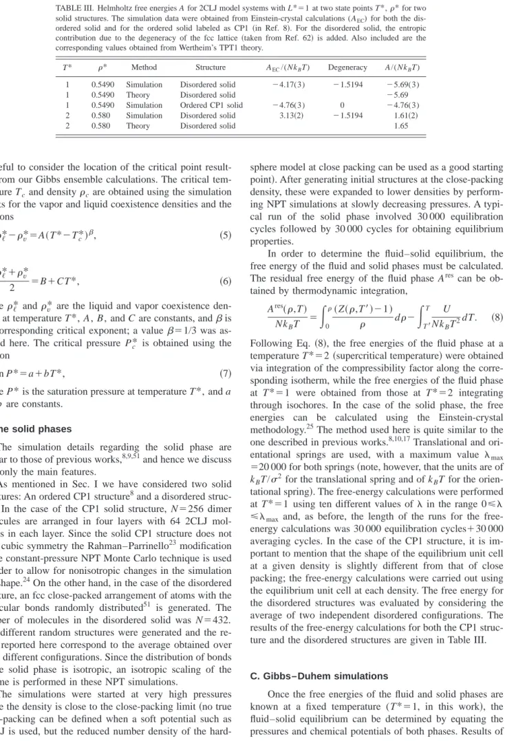
Once the free energies of the fluid and solid phases are known at a fixed temperature (T*⫽1, in this work兲, the fluid–solid equilibrium can be determined by equating the pressures and chemical potentials of both phases. Results of TABLE III. Helmholtz free energies A for 2CLJ model systems with L*⫽1 at two state points T*,*for two
solid structures. The simulation data were obtained from Einstein-crystal calculations (AEC) for both the
dis-ordered solid and for the dis-ordered solid labeled as CP1共in Ref. 8兲. For the disordered solid, the entropic contribution due to the degeneracy of the fcc lattice共taken from Ref. 62兲is added. Also included are the corresponding values obtained from Wertheim’s TPT1 theory.
T* * Method Structure AEC/(NkBT) Degeneracy A/(NkBT)
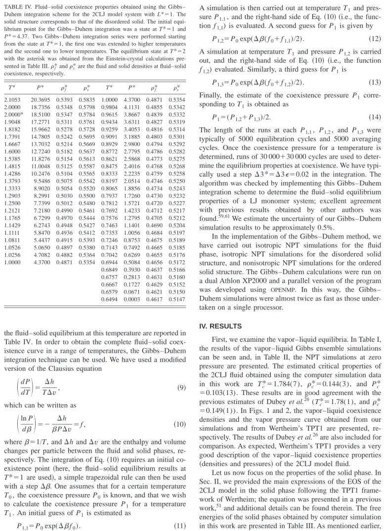
the fluid–solid equilibrium at this temperature are reported in Table IV. In order to obtain the complete fluid–solid coex-istence curve in a range of temperatures, the Gibbs–Duhem integration technique can be used. We have used a modified version of the Clausius equation
冉
d P dT冊
⫽⌬h
T⌬v, 共9兲
which can be written as
冉
ln Pd
冊
⫽⫺⌬h
P⌬v⫽f , 共10兲
where⫽1/T, and⌬h and⌬vare the enthalpy and volume changes per particle between the fluid and solid phases, re-spectively. The integration of Eq.共10兲requires an initial co-existence point 共here, the fluid–solid equilibrium results at T*⫽1 are used兲, a simple trapezoidal rule can then be used with a step ⌬. One assumes that for a certain temperature T0, the coexistence pressure P0 is known, and that we wish
to calculate the coexistence pressure P1 for a temperature
T1. An initial guess of P1 is estimated as
P1,1⫽P0exp共⌬f0兲. 共11兲
A simulation is then carried out at temperature T1 and
pres-sure P1,1, and the right-hand side of Eq.共10兲 共i.e., the
func-tion f1,1) is evaluated. A second guess for P1 is given by
P1,2⫽P0exp共⌬共f0⫹f1,1兲/2兲. 共12兲
A simulation at temperature T1 and pressure P1,2 is carried
out, and the right-hand side of Eq. 共10兲 共i.e., the function f1,2) evaluated. Similarly, a third guess for P1 is
P1,3⫽P0exp共⌬共f0⫹f1,2兲/2兲. 共13兲
Finally, the estimate of the coexistence pressure P1
corre-sponding to T1 is obtained as
P1⫽共P1,2⫹P1,3兲/2. 共14兲
The length of the runs at each P1,1, P1,2, and P1,3 were
typically of 5000 equilibration cycles and 5000 averaging cycles. Once the coexistence pressure for a temperature is determined, runs of 30 000⫹30 000 cycles are used to deter-mine the equilibrium properties at coexistence. We have typi-cally used a step ⌬3*⫽⌬3⑀⫽0.02 in the integration. The algorithm was checked by implementing this Gibbs–Duhem integration scheme to determine the fluid–solid equilibrium properties of a LJ monomer system; excellent agreement with previous results obtained by other authors was found.59,61We estimate the uncertainty of our Gibbs–Duhem simulation results to be approximately 0.5%.
In the implementation of the Gibbs–Duhem method, we have carried out isotropic NPT simulations for the fluid phase, isotropic NPT simulations for the disordered solid structure, and nonisotropic NPT simulations for the ordered solid structure. The Gibbs–Duhem calculations were run on a dual Athlon XP2000 and a parallel version of the program was developed using OPENMP. In this way, the Gibbs– Duhem simulations were almost twice as fast as those under-taken on a single processor.
IV. RESULTS
First, we examine the vapor–liquid equilibria. In Table I, the results of the vapor–liquid Gibbs ensemble simulations can be seen and, in Table II, the NPT simulations at zero pressure are presented. The estimated critical properties of the 2CLJ fluid obtained using the computer simulation data in this work are Tc*⫽1.784(7), c*⫽0.144(3), and Pc* ⫽0.103(13). These results are in good agreement with the previous estimates of Dubey et al.26 (Tc*⫽1.78(1), andc* ⫽0.149(1)). In Figs. 1 and 2, the vapor–liquid coexistence densities and the vapor pressure curve obtained from our simulations and from Wertheim’s TPT1 are presented, re-spectively. The results of Dubey et al.26are also included for comparison. As expected, Wertheim’s TPT1 provides a very good description of the vapor–liquid coexistence properties
共densities and pressures兲of the 2CLJ model fluid.
Let us now focus on the properties of the solid phase. In Sec. II, we provided the main expressions of the EOS of the 2CLJ model in the solid phase following the TPT1 frame-work of Wertheim; the equation was presented in a previous work,51and additional details can be found therein. The free energies of the solid phases obtained by computer simulation in this work are presented in Table III. As mentioned earlier, TABLE IV. Fluid–solid coexistence properties obtained using the Gibbs–
Duhem integration scheme for the 2CLJ model system with L*⫽1. The solid structure corresponds to that of the disordered solid. The initial equi-librium point for the Gibbs–Duhem integration was a state at T*⫽1 and
P*⫽4.37. Two Gibbs–Duhem integration series were performed starting from the state at T*⫽1, the first one was extended to higher temperatures and the second one to lower temperatures. The equilibrium state at T*⫽2 with the asterisk was obtained from the Einstein-crystal calculations pre-sented in Table III.f*ands*are the fluid and solid densities at fluid–solid
coexistence, respectively.
T* P* f* s* T* P* f* s*
in the case of the disordered solid structure, the results cor-respond to the average of two independent disordered con-figurations. In Table III, the calculated free energies using Wertheim’s TPT1 have also been included. It can be seen that the theoretical approach provides accurate predictions of the free energy of the disordered solid. It is important to note here that, in order to obtain the free energy of the disordered solid, the contribution of the degeneracy entropy must be added to the free energy obtained from the Einstein-crystal calculations. This is due to the fact that this method provides the free energy associated with a given solid configuration and, therefore, the degeneracy entropy must be added to ac-count for the number of ways of organizing a disordered solid configuration. In the case of dimer molecules on an fcc
lattice, the estimation of the number of ways of arranging the configuration is known as the ‘‘dimer problem.’’ Nagle62 pro-posed an accurate estimate of the degeneracy entropy giving A/(NkBT)⫽⫺1.5194. It is clear from Table III that, for a given density, the free energy of the disordered solid is lower than that of the ordered CP1 solid, meaning that the stable solid structure for the 2CLJ model corresponds to the disor-dered solid and not to the ordisor-dered CP1 solid. This was first shown in a two-dimensional hard-disk dimer system by Wojciechowski et al.;52,53our results indicate that the same conclusion holds true in the case of a three-dimensional 2CLJ solid. It is important to note, however, that 共stable兲 disordered structures are not possible for values of L* sig-nificantly different from unity. For values of L*less than 1, the stable solid phase is expected to exhibit an ordered struc-ture; i.e., the singular nature of the model with L*⫽1 makes the existence of the disordered solid possible.
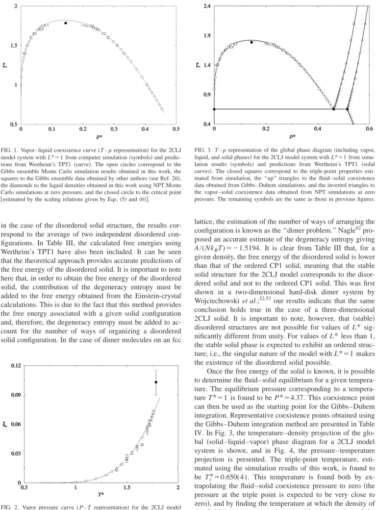
Once the free energy of the solid is known, it is possible to determine the fluid–solid equilibrium for a given ture. The equilibrium pressure corresponding to a tempera-ture T*⫽1 is found to be P*⫽4.37. This coexistence point can then be used as the starting point for the Gibbs–Duhem integration. Representative coexistence points obtained using the Gibbs–Duhem integration method are presented in Table IV. In Fig. 3, the temperature–density projection of the glo-bal 共solid–liquid–vapor兲 phase diagram for a 2CLJ model system is shown, and in Fig. 4, the pressure–temperature projection is presented. The triple-point temperature, esti-mated using the simulation results of this work, is found to be Tt*⫽0.650(4). This temperature is found both by ex-trapolating the fluid–solid coexistence pressure to zero 共the pressure at the triple point is expected to be very close to zero兲, and by finding the temperature at which the density of the fluid at zero pressure becomes identical to that of the fluid at the fluid–solid coexistence curve. The corresponding FIG. 1. Vapor–liquid coexistence curve (T –representation兲for the 2CLJ
model system with L*⫽1 from computer simulation共symbols兲and predic-tions from Wertheim’s TPT1 共curve兲. The open circles correspond to the Gibbs ensemble Monte Carlo simulation results obtained in this work, the squares to the Gibbs ensemble data obtained by other authors共see Ref. 26兲, the diamonds to the liquid densities obtained in this work using NPT Monte Carlo simulations at zero pressure, and the closed circle to the critical point
关estimated by the scaling relations given by Eqs.共5兲and共6兲兴.
FIG. 2. Vapor pressure curve ( P – T representation兲 for the 2CLJ model system with L*⫽1 from computer simulation 共symbols兲 and predictions from Wertheim’s TPT1共curve兲. See Fig. 1 for details of the symbols.
coexistence densities at the triple point are *f⫽0.462, and
s*⫽0.515. In Figs. 3 and 4, the results obtained using the equations based on Wertheim’s TPT1 are also included. It is clearly seen that the theory provides an accurate description of the coexistence properties of the 2CLJ model, including the fluid–solid equilibria. The theory predicts a triple point at Tt*⫽0.653, in excellent agreement with the simulation re-sult. The triple-point temperature in a LJ monomer system predicted by the theory共i.e., m⫽1 here兲 is found to be Tt* ⫽0.687, which is also in excellent agreement with the com-puter simulation estimate of Agrawal and Kofke61 (Tt* ⫽0.687). As can be seen, the triple-point temperature of the LJ dimer is 5% lower than that of the LJ monomer. The comparison can be seen more clearly in Fig. 5, where the phase diagram of the monomer LJ and of the 2CLJ model
systems are shown. Note that in the Fig. 5, the density is expressed as the number of monomers per unit volume.
It is also useful to compare these results with those of the case in which the ordered structure of 2CLJ molecules is considered to be the stable phase. In Fig. 6, the phase dia-gram in such a case is presented. Results for the fluid-ordered solid transition found from Gibbs–Duhem simula-tions are presented in Table V. The triple point in this case would be located at Tt⫽0.534(5). The lower stability of the ordered phase provokes a decrease in the triple-point tem-perature, shifting the fluid–solid equilibrium to higher den-sities. The triple-point temperature of the 2CLJ model sys-tem with L*⫽0.67 has been determined by Lisal and FIG. 4. P – T representation of the global phase diagram共vapor, liquid, and
solid phases兲for the 2CLJ model system with L*⫽1 from simulation re-sults共symbols兲and Wertheim’s TPT1共solid curves兲. See Fig. 3 for details of the symbols. The inset shows the P – T diagram at high pressure.
FIG. 5. T –representation of the global phase diagram共vapor, liquid, and solid phases兲of the LJ system共solid curves兲, and that of the 2CLJ model system with L*⫽1共dashed curves兲. The reduced number density of mono-mers is denoted asm*⫽m*.
FIG. 6. T –representation of the global phase diagram of the 2CLJ system obtained in this work from Gibbs–Duhem simulations in the case of an ordered CP1 solid phase. The symbols have the same meaning as those in Fig. 3.
TABLE V. Fluid–solid coexistence conditions obtained using the Gibbs– Duhem integration method for a 2CLJ model system with L*⫽1. The solid structure corresponds to that of the ordered CP1 solid. The initial equilib-rium point for the Gibbs–Duhem integration was a state at T*⫽1 and P* ⫽11.10. The density at coexistence of the fluid is denoted as*f , whereas
that of the solid is denoted ass*.
T* P* f* s*
Vacek36at Tt*⫽0.62共in this case, the stable structure of the solid is the ordered one兲. When compared to the critical point, the ratio Tt/Tc in the system with L*⫽0.67 takes a value Tt/Tc⫽0.27, while for the model with L*⫽1 this ra-tio takes a value Tt/Tc⫽0.36 when the共stable兲 disordered structure is considered, and Tt/Tc⫽0.30 when the ordered CP1 structure is assumed. These calculations show that for the ordered solid, the ratio Tt/Tc is roughly constant with a value of about 0.27, and slowly increases with L*. This con-clusion holds for systems with bond lengths L*⬎0.4 共no plastic crystal phases are possible兲.63A marked difference is noted in comparison with the Tt/Tcratio of the LJ monomer fluid (Tt/Tc⫽0.687/1.31⫽0.52). In summary, the triple-point temperature is about 0.3 of the critical triple-point in the case of 2CLJ fluids with L*⬎0.4, but it is 1/2 of the critical temperature in monomer LJ fluids. More work is needed to assess the variation of Tt/Tcwith L*, especially in the range of small values of L* where plastic crystal phases are pos-sible. However, the results of this work allow one to obtain a tentative value for the ratio Tt/Tcof 2CLJ models of varying L*. This is presented in Fig. 7. The results of this work are in line with the predictions of the mean-field theory proposed by Paras et al.63
Let us finish by discussing the phase behavior of the 2CLJ at very low temperatures. For the range of tempera-tures considered so far 共above the triple point兲, the disor-dered solid phase was found to be the stable phase. However, it is not clear which is the stable solid phase at very low temperatures, since the ordered and disordered solids have different thermodynamic properties. The differences may be summarized as follows. For a certain temperature and den-sity, the ordered solid has a slightly higher pressure, and a slightly lower internal energy, than the disordered solid. Zero-pressure densities of the ordered solid are slightly smaller than those of the disordered solid. The differences
are small, but clearly visible. Simulations results for ordered and disordered solids were presented in tabular form in Ref. 51 and shall not be reproduced here. In order to evaluate the free energy of the ordered and disordered solid phases at low temperatures, we have performed NVT simulations of the solid phase at constant density*⫽0.549共using the equilib-rium shape of the unit cell兲, starting at temperature T*⫽1 and ending at T*⫽0.20. Thermodynamic integration yields the following expression for the free energies of the solid phase along the isochore:
A
NkBT共
*⫽0.549,T*兲⫽ A
NkBT共
*⫽0.549,T*⫽1兲
⫺
冕
1
T* U
N⑀共T*兲2dT*. 共15兲
To perform the integral of Eq. 共15兲, we have fitted the residual internal energy to the following expression:
U
N⑀⫽c0⫹c1T*⫹c2共T*兲
2⫹c
3共T*兲3⫹c4共T*兲4. 共16兲
The values of coefficients c0⫺c4 from Eq. 共16兲,
corre-sponding to the ordered solid, are ⫺16.538, 2.3769,
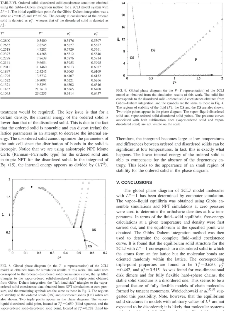
⫺0.074 064, ⫺0.141 85, and 0.090 332, whereas those for the disordered solid are ⫺16.223, 2.5488, ⫺0.38 096, 0.271 78, and ⫺0.116 38. The values of the free energy at the reference state defined by *⫽0.549 and T*⫽1 for the ordered and disordered solids were taken from Table III. It was found that the Helmholtz free energies of the ordered and disordered solids were identical for *⫽0.549 and T* ⫽0.28. NPT simulations were performed for both the or-dered and disoror-dered solids at T*⫽0.28, and the EOS and chemical potentials were evaluated for both types of solids. It was found that at low pressures, the ordered solid was more stable共lower chemical potential for a certain pressure兲 than the disordered solid. At high pressures, the disordered solid turns out to be the stable phase. We locate the first-order phase transition between the first-ordered and the disor-dered solid phase at P*⫽0.54 for T*⫽0.28. Taking this state as the initial equilibrium point, Gibbs–Duhem integra-tion was performed in order to evaluate the coexistence line between the ordered and the disordered solid. Results are presented in Table VI and Figs. 8 and 9. As can be seen, the ordered solid is indeed the stable phase at low temperatures and pressures. The vapor-ordered solid-disordered solid triple point is located at T*⫽0.282, the densities of the or-dered and disoror-dered solids being o*⫽0.5433 and d* ⫽0.5462, respectively. It is noticeable in Fig. 8 that the den-sity jump between the two solid phases is small, and in Fig.9 that the slope of the ordered solid–disordered solid phase transition is negative. Using the Clapeyron relation, it can be shown that the negative slope follows from a negative value of ⌬v 共the disordered solid has a higher density than the ordered one兲and a positive value of⌬h 共the disordered solid has a higher enthalpy than the ordered solid兲. Is it possible to provide a simple explanation for the fact that the ordered solid is the stable phase at low temperatures? Notice that we are using classical statistical thermodynamics here共although for a real substance at such low temperatures, a quantum FIG. 7. Sketch of the Tt/Tcratio for 2CLJ model systems.共See Refs. 61
and 36, respectively, for the results for L*⫽0 and those corresponding to
treatment would be required兲. The key issue is that for a certain density, the internal energy of the ordered solid is lower than that of the disordered solid. This is due to the fact that the ordered solid is noncubic and can distort共relax兲the lattice parameters in an attempt to decrease the internal en-ergy. The disordered solid cannot optimize the parameters of the unit cell since the distribution of bonds in the solid is isotropic. Notice that we are using anisotropic NPT Monte Carlo 共Rahman–Parrinello type兲 for the ordered solid and isotropic NPT for the disordered solid. In the integrand of Eq. 共15兲, the internal energy appears as divided by (1/T2).
Therefore, the integrand becomes large at low temperatures and differences between ordered and disordered solids can be significant at low temperatures. In fact, this is exactly what happens. The lower internal energy of the ordered solid is able to compensate for the absence of the degeneracy en-tropy. This leads to the appearance of an small region of stability for the ordered solid in the phase diagram.
V. CONCLUSIONS
The global phase diagram of 2CLJ model molecules with L*⫽1 has been determined by computer simulation. The vapor–liquid equilibria was obtained using Gibbs en-semble simulations and NPT simulations at zero pressure were used to determine the orthobaric densities at low tem-peratures. In terms of the fluid–solid equilibria, free-energy calculations at a given temperature and density were first carried out, and the equilibrium at the specified point was obtained. The Gibbs–Duhem integration method was then used to determine the complete fluid–solid coexistence curve. It is found that the equilibrium solid structure for the 2CLJ with L*⫽1 corresponds to a disordered solid in which the atoms form an fcc lattice but the molecular bonds are oriented randomly within the lattice. The corresponding triple-point properties are found to be Tt*⫽0.650, *f ⫽0.462, ands*⫽0.515. As was found for two-dimensional disk dimers and for fully flexible hard-sphere chains, the stable solid structure is a disordered one. This seems to be a general feature of fully flexible models of chain molecules formed by tangent monomers. Wojciechowski et al.52,53 sug-gested this possibility. Note, however, that the equilibrium solid structures in models with arbitrary values of L*are not expected to be disordered; it is likely that molecular systems with a bond length L* different from 1 will exhibit ordered TABLE VI. Ordered solid–disordered solid coexistence conditions obtained
using the Gibbs–Duhem integration method for a 2CLJ model system with
L*⫽1. The initial equilibrium point for the Gibbs–Duhem integration was a state at T*⫽0.28 and P*⫽0.54. The density at coexistence of the ordered solid is denoted aso*, whereas that of the disordered solid is denoted as d*.
T* P* o* d*
0.2800 0.5400 0.5476 0.5507 0.2652 2.8245 0.5627 0.5657 0.2518 4.7287 0.5729 0.5761 0.2397 6.4268 0.5812 0.5846 0.2288 7.8639 0.5876 0.5914 0.2141 9.6654 0.5953 0.5995 0.2011 11.1460 0.6013 0.6057 0.1897 12.4245 0.6063 0.6109 0.1795 13.5732 0.6107 0.6152 0.1522 16.8007 0.6221 0.6266 0.1321 19.3293 0.6302 0.6346 0.1167 21.3610 0.6365 0.6408 0.1045 23.0255 0.6414 0.6457
FIG. 8. Global phase diagram 共in the T – representation兲 of the 2CLJ model as obtained from the simulation results of this work. The solid lines correspond to the ordered–disordered solid coexistence curve, the up filled triangles to the vapor-ordered solid-disordered solid triple-point obtained from Gibbs–Duhem integration, the ‘‘left-hand side’’ triangles to the vapor-ordered solid coexistence data obtained from NPT simulations at zero pres-sure, and the remaining symbols are the same as those in Fig. 3. The regions of stability of the ordered solids共OS兲and disordered solids共DS兲solids are also shown. Two triple points appear in the phase diagram: The vapor– liquid-disordered solid point, located at Tt*⫽0.650共filled squares兲, and the
vapor-ordered solid-disordered solid point, located at Tt*⫽0.282共filled
tri-angles兲.
structures as the stable solid phases. We have shown that Wertheim’s TPT1 can be used to study both fluid and solid phases of chainlike LJ molecules. The theoretical approach provides not only an accurate EOS, but also accurate values of the free energies for both fluid and solid phases. As a result, we have been able to show the excellent agreement found between the computer simulation phase equilibrium data and the calculated phase diagram for the 2CLJ model system, including the vapor–liquid–solid triple point. This article validates the fact that Wertheim’s TPT1 can be used to predict phase diagrams of fully flexible LJ chains as was first shown in Ref. 51. By comparing the triple-point temperature Ttof the 2CLJ with that of the monomer, it is found that the dimer system has a Tt 5% lower than that of the monomer system.
The fluid–solid equilibrium between the fluid and an ordered solid has also been obtained by means of computer simulations. In this case, the triple point is found at Tt* ⫽0.534, which means that the ratio Tt/Tc⫽0.30 for the or-dered solid with L*⫽1. Lisal and Vacek36 evaluated this ratio for a system with L*⫽0.67 obtaining Tt/Tc⫽0.27. It seems that in 2CLJ systems, the ratio Tt/Tcslowly increases with L*in the region where the stable solid phase is ordered, i.e., 0.4⭐L*⬍1, as was predicted some time ago using a mean-field approach.63
For the model considered here, the 2CLJ with L*⫽1, the disordered solid was found to be the stable solid phase for most of thermodynamic conditions. However, it has been found that at very low temperatures共substantially below the triple point兲, the stable solid phase is an ordered solid. The lower internal energy of the ordered solid is able to compen-sate for the absence of the degeneracy entropy leading to the appearance of an small region of stability for the ordered solid.
ACKNOWLEDGMENTS
Financial support is due to project Nos. BFM-2001-1420-C02-01 and BFM-2001-1420-C02-02 of Spanish DGI-CYT 共Direccio´n General de Investigacio´n Cientı´fica y Te´c-nica兲. One of the authors共A.G.兲would also like to thank the Engineering and Physical Sciences Research Council for the award of an Advanced Research Fellowship. E.d.M. and F.J.B. also acknowledge the Junta de Andalucia and Univer-sidad de Huelva for additional financial support.
1W. G. Hoover and F. H. Ree, J. Chem. Phys. 49, 3609共1968兲.
2B. J. Alder, W. G. Hoover, and D. A. Young, J. Chem. Phys. 49, 3688
共1968兲.
3J. P. Hansen and L. Verlet, Phys. Rev. 184, 151共1969兲. 4
D. Frenkel and B. M. Mulder, Mol. Phys. 55, 1171共1985兲.
5P. Bolhuis and D. Frenkel, J. Chem. Phys. 106, 666共1997兲. 6J. A. C. Veerman and D. Frenkel, Phys. Rev. A 45, 5632共1992兲. 7S. J. Singer and R. J. Mumaugh, J. Chem. Phys. 93, 1278共1990兲. 8
C. Vega, E. P. A. Paras, and P. A. Monson, J. Chem. Phys. 96, 9060
共1992兲.
9C. Vega, E. P. A. Paras, and P. A. Monson, J. Chem. Phys. 97, 8543
共1992兲.
10C. Vega and P. A. Monson, J. Chem. Phys. 102, 1361共1995兲. 11A. P. Malanoski and P. A. Monson, J. Chem. Phys. 107, 6899共1997兲. 12P. A. Monson and D. A. Kofke, Adv. Chem. Phys. 115, 113共2000兲. 13C. Vega, F. Bresme, and J. L. F. Abascal, Phys. Rev. E 54, 2746共1996兲. 14F. Bresme, C. Vega, and J. L. F. Abascal, Phys. Rev. Lett. 85, 3217共2000兲. 15
B. Smit, K. Esselink, and D. Frenkel, Mol. Phys. 87, 159共1996兲.
16E. de Miguel, L. F. Rull, M. K. Chalam, and K. E. Gubbins, Mol. Phys.
74, 405共1991兲.
17E. de Miguel and C. Vega, J. Chem. Phys. 117, 6313共2002兲. 18
L. A. Baez and P. Clancy, J. Chem. Phys. 103, 9744共1995兲.
19A. Z. Panagiotopoulos, Mol. Phys. 61, 813共1987兲. 20
A. Lotfi, J. Vrabec, and J. Fischer, Mol. Phys. 76, 1319共1992兲.
21D. A. Kofke, Mol. Phys. 78, 1331共1993兲. 22
D. A. Kofke, J. Chem. Phys. 98, 4149共1993兲.
23M. Parrinello and A. Rahman, Phys. Rev. Lett. 45, 1196共1980兲. 24
S. Yashonath and C. N. R. Rao, Mol. Phys. 54, 245共1985兲.
25D. Frenkel and A. J. C. Ladd, J. Chem. Phys. 81, 3188共1984兲. 26
G. S. Dubey, S. O’Shea, and P. A. Monson, Mol. Phys. 80, 997共1993兲.
27G. Galasi and D. J. Tildesley, Mol. Simul. 13, 11共1994兲. 28
J. Stoll, J. Vrabec, H. Hasse, and J. Fischer, Fluid Phase Equilibria 179, 339共2001兲.
29
M. Lisal, R. Budinsky, and V. Vacek, Fluid Phase Equilibria 135, 193
共1997兲.
30C. Kriebel, A. Muller, J. Winkelmann, and J. Fischer, Mol. Phys. 84, 381
共1995兲.
31M. Lombardero, J. L. F. Abascal, and S. Lago, Mol. Phys. 42, 999共1981兲. 32J. Fischer, J. Chem. Phys. 72, 5371共1980兲.
33D. B. McGuigan, M. Lupkowski, D. M. Paquet, and P. A. Monson, Mol.
Phys. 67, 33共1989兲.
34J. Fischer, R. Lustig, M. Breitenfelder-Manske, and W. Lemming, Mol.
Phys. 52, 485共1984兲.
35C. T. Lin and G. Stell, J. Chem. Phys. 114, 6969共2001兲. 36M. Lisal and V. Vacek, Mol. Simul. 19, 43共1997兲. 37M. S. Wertheim, J. Stat. Phys. 35, 19共1984兲. 38M. S. Wertheim, J. Stat. Phys. 35, 35共1984兲. 39M. S. Wertheim, J. Stat. Phys. 42, 459共1986兲. 40
M. S. Wertheim, J. Stat. Phys. 42, 477共1986兲.
41M. S. Wertheim, J. Chem. Phys. 87, 7323共1987兲. 42
W. G. Chapman, G. Jackson, and K. E. Gubbins, Mol. Phys. 65, 1057
共1988兲.
43
W. G. Chapman, J. Chem. Phys. 93, 4299共1990兲.
44J. K. Johnson, J. A. Zollweg, and K. E. Gubbins, Mol. Phys. 78, 591
共1993兲.
45J. K. Johnson, E. A. Muller, and K. E. Gubbins, J. Phys. Chem. 98, 6413
共1994兲.
46F. J. Blas and L. F. Vega, Mol. Phys. 92, 1共1997兲. 47
F. J. Blas and L. F. Vega, J. Chem. Phys. 115, 4355共2001兲.
48C. Vega and L. G. MacDowell, J. Chem. Phys. 114, 10411共2001兲. 49
F. J. Blas, A. Galindo, and C. Vega, Mol. Phys. 101, 449共2003兲.
50C. McBride and C. Vega, J. Chem. Phys. 116, 1757共2002兲. 51
C. Vega, F. J. Blas, and A. Galindo, J. Chem. Phys. 116, 7645共2002兲.
52K. W. Wojciechowski, A. C. Branka, and D. Frenkel, Physica A 196, 519
共1993兲.
53K. W. Wojciechowski, D. Frenkel, and A. C. Branka, Phys. Rev. Lett. 66,
3168共1991兲.
54E. A. Muller and K. E. Gubbins, Ind. Eng. Chem. Res. 40, 2193共2001兲. 55J. P. Hansen and I. R. McDonald, Theory of Simple Liquids共Academic,
New York, 1986兲.
56D. A. McQuarrie, Statistical Mechanics 共Harper and Row, New York,
1976兲.
57R. P. Sear and G. Jackson, J. Chem. Phys. 102, 939共1995兲.
58N. Elvassore and J. M. Prausnitz, Fluid Phase Equilibria 194, 567共2002兲. 59M. A. van der Hoef, J. Chem. Phys. 113, 8142共2000兲.
60M. P. Allen and D. J. Tildesley, Computer Simulation of Liquids, 2nd ed.
共Clarendon, Oxford, 1987兲.
61R. Agrawal and D. A. Kofke, Mol. Phys. 85, 43共1995兲. 62J. F. Nagle, Phys. Rev. 152, 190共1966兲.