Operational Modal Analysis using Expectation Maximization Algorithm
F.J. Cara1, J. Carpio1, J. Juan1, E. Alarcon2
1Department of Organization Engineering, Business Administration and Statistics,
E.T.S.I. Industriales U.P.M., Jose Gutierrez Abascal 2, 28080 Madrid, Spain
2Department of Structural Mechanics and Industrial Constructions
E.T.S.I. Industriales U.P.M., Jose Gutierrez Abascal 2, 28080 Madrid, Spain
email: [email protected], [email protected], [email protected], [email protected]
ABSTRACT: This paper presents a time-domain stochastic system identification method based on Maximum Likelihood Estimation and the Expectation Maximization algorithm. The effectiveness of this structural identification method is evaluated through numerical simulation in the context of the ASCE benchmark problem on structural health monitoring. Modal parameters (eigenfrequencies, damping ratios and mode shapes) of the benchmark structure have been estimated applying the proposed identification method to a set of 100 simulated cases. The numerical results show that the proposed method estimates all the modal parameters reasonably well in the presence of 30% measurement noise even. Finally, advantages and disadvantages of the method have been discussed.
KEY WORDS: System identification in structures, State Space models, Kalman filter, Operational Modal analysis, Maximum likelihood estimation, Expectation Maximization algorithm.
1 INTRODUCTION
The application of system identification to vibrating structures consist in identifying a modal model (eigenfrequencies, damp-ing ratios and mode shapes) from vibration data. Classically, a measurable input is applied to the system and the output is measured. From these experimental data, a system model can be obtained by a variety of parameter estimation methods, and it is known as experimental modal analysis. However, cases exist where it is practically impossible to measure the excitation and the outputs are the only information that is passed to the system identification algorithms. In these cases the deterministic knowledge of the input is replaced by the assumption that the input is a realization of a stochastic process (white noise), and it is known as stochastic system identification (the terms output-only modal analysis and operational modal analysis are used as well).
Parametric structural identification methods involve the use of mathematical models to represent structural system behaviour in either time or frequency domain. The benefits of using parametric models for structural identification include their direct relationship with physically meaningful quantities such as stiffness and mass, improved accuracy and resolution, and their suitability for analysis, prediction, fault diagnosis and control.
Popular time domain parametric models used for structural identification purposes include: ARX models, ARMAX models, state space models, etc. Many identification algorithms are available to estimate the parameters of such parametric models, e.g. prediction error method (PEM), least squares estimation (LSE), maximum likelihood estimation (MLE), eigensystem re-alization algorithm (ERA) and stochastic subspace identification method (SSI).
This paper presents a time-domain stochastic system iden-tification method based on Maximum Likelihood Estimation (MLE) and the Expectation Maximization (EM) algorithm. The results of this structural identification method are evaluated through numerical simulation in the context of the ASCE benchmark problem on structural health monitoring [1]. The modal parameters (eigenfrequencies, damping ratios and mode shapes) of the benchmark structure (see Figure 1) have been estimated using the proposed MLE+EM method and then have been compared to the exact values.
2 STATE-SPACE MODEL
2.1 Stochastic state-space equations
The equations of motion for annd degrees-of-freedom (DOF)
linear, time invariant, viscously damped system subjected to external excitation is expressed as
Mz¨(t) +Cζz˙(t) +Kz(t) =Ju(t) (1)
whereM,Cζ,K∈Rnd×nd are the mass, damping and stiffness
matrices, respectively; J ∈Rnd×ni is the excitation influence
matrix that relates theni-dimensional input vectoru(t) to the
nd-dimensional response vector; z(t) is the nd-dimensional
displacement response vector; dot denotes taking derivatives with respect to time.
By defining the state vectorx(t) = [z(t)z˙(t)]T, equation (1) can be converted into the continuous state space form
˙
x(t) =Acx(t) +Bcu(t) (2)
where
Ac=
0 I
−M−1K −M−1Cζ
Bc=
0 M−1J
In practice, only a limited number of measurements are available; therefore, the dimension of the measurement output is less than or equal to the total number of degrees of freedom. Theno-dimensional output vectory(t)can be expressed as
y(t) =Cd(t)z(t) +Cvz˙(t) +Caz¨(t) (4)
where Cd,Cv,Ca ∈ Rno×nd are the measurement location
matrices corresponding to the displacement, velocity and acceleration responses of the structural system, respectively. We can rewrite the output vector into the continuous state space form,
y(t) =Ccx(t) +Dcu(t) (5)
where
Cc= [Cd−CaM−1K Cv−CaM−1Cζ] Dc=CaM−1J (6)
In this work, only accelerations are considered, so
Cc=Ca[−M−1K −M−1Cζ] (7)
Equations 2 and 5 define the state space equation in continuous time:
˙
x(t) =Acx(t) +Bcu(t) (8a)
y(t) =Ccx(t) +Dcu(t) (8b)
where
y(t)∈Rnois the measuredoutput vector;
u(t)∈Rni is the measuredinput vector;
x(t)∈Rnsis thestate vector;
Ac ∈ Rns×ns is the transition state matrix describing the
dynamics of the system; Bc∈Rns×niis theinput matrix;
Cc∈Rno×ns is theoutput matrix, which is describing how the
internal state is transferred to the the output measurementsy(t);
Dc∈Rno×ni is thedirect transmission matrix;
Equation (8a) is known as the State Equationand equation (8b) is known as theObservation Equation.
But measurements are taken in discrete time instants, so equations must be expressed in discrete time too. Typical for the sampling of a continuous-time equation is a Zero-Order Hold assumption, which means that the input is piecewise constant over the sampling period, that is
∀t∈[tk,tk+1) = [k∆t,(k+1)∆t) =⇒
x(t) =x(tk) =xk,u(t) =u(tk) =uk,y(t) =y(tk) =yk (9)
Under this assumption, the continuous time state-space model (8a) and (8b) is converted to the discrete time state-space model:
xk+1=Axk+Buk (10a)
yk=Cxk+Duk (10b)
wherexkis the discrete time state vector containing the sampled
displacements and velocities; uk andyk are the sampled input
and output;Ais the discrete state matrix;Bis the discrete input matrix;Cis the discrete output matrix;Dis the discrete direct transmission matrix. They are related to their continuous-time counterparts as (see for instance [2]):
A=eAc∆t (11)
B= (A−I)A−c1Bc (12)
C=Cc (13)
D=Dc (14)
Up to now it was assumed that the system was only driven by a deterministic input uk. However, besides this applied
input there might be other inputs that in a more uncontrollable way contribute to the system response. This unmeasurable influence is characterized as disturbance or noise. In system identification, system response disturbance might be caused by different phenomena. The most obvious one is noise generated by the sensors, or noise arising from roundoff errors during A/D conversion. In any case, noise will always be present in measured data and should be therefore always take into account. It is necessary to extend the state space model (10a) and (10b) including stochastic components, sostochastic state space modelis obtained:
xk+1=Axk+Buk+wk (15a)
yk=Cxk+Duk+vk (15b)
wherewk ∈Rns is the process noise due to disturbances and
modeling inaccuracies;vk∈Rno is the measurement noise due
to sensor inaccuracy. We assume they are both independent and identically distributed, zero-mean normal vectors
wk;N(0,Q) uk;N(0,R) (16)
In the case of ambient vibration testing, only the responses of the structureyk are measured, while the input sequence uk
remains unmeasured. Equations (15a) and (15b) result now in a purely stochastic system:
xk+1=Axk+wk (17a)
yk=Cxk+vk (17b)
The input is now implicitly modeled by the noise terms wk,
vk. However the white noise assumptions of these noise terms
cannot be omitted and (16) remain still applicable in equation (17).
2.2 The Kalman filter
Due to the noise present in the stochastic state space Equations (17), it is only possible to predict the response in term of probability. For state space systems, this prediction is accomplished by the construction of the associated Kalman filter.
The Kalman filter is a computational scheme to estimate the states of a given state-space model in a statistically optimal manner. This filter is derived in a framework based on conditional probability theory, and the theoretical foundations used from statistics are complex.
The following notation will be used in all the expressions where the Kalman filter is involved. Given the output data fors time stepsYs={y1,y2, . . . ,ys}, it is defined:
xts=E[xt|Ys]
Ps
t1,t2=E(xt1−xst1)(xt2−xst2) T|Y
where E[•|•]is the conditional expected operator. Whent1=
t2=t,Pts1,t2 will be writtenPts:
Pts=E(xt−xst)(xt−xst)T|Ys=Var[xt|Ys]
Property 1(The Kalman Filter) For the state space model specified in (17) with initial conditions x0
0=µ0andP00=Σ0,
fork=1,2, . . . ,N,
xk−1
k =Axkk−−11 (18)
Pk−1
k =APkk−−11AT+Q (19)
with
xk
k=xkk−1+Kkεk (20)
Pk
k = (I−KkC)Pkk−1 (21)
where
Kk=Pkk−1CTΣ−k1 (22)
εk=yk−E[yk|Yk−1] =yk−Cxkk−1 (23)
Σk=Var(εk) =Var[C(xk−xkk−1) +vk] =CPkk−1CT+R (24)
Kkis called the Kalman gain andεkare the innovations.
The demonstration of the above property can be found in [3].
2.3 The innovation form representation
An alternative model for stochastic systems that is more suitable for some applications is the so-calledinnovation form representation. It is obtained applying the the Kalman filter to the stochastic state-space model (17):
xk−1
k =Axkk−−11=A
xk−2
k−1+Kk−1εk−1
=Axkk−−21+AKk−1εk−1
(25) so
xkk+1=Axkk−1+AKkεk (26a)
yk=Cxkk−1+εk (26b)
whereKk is the Kalman gain (22) andεk are the innovations
(23).
Under stationary conditions (see for instance [4]),
lim
k→∞P
k−1
k =P>0 (27)
and the innovation form representation converges to the following time-invariant state-space system:
xk
k+1=Axkk−1+Kεk (28a)
yk=Cxkk−1+εk (28b)
where
P=APAT+Q−APCT(CPCT+R)−1(APCT)T (29)
K=APCT(CPCT+R)−1 (30)
Equation 29 is called a discrete algebraic Riccati equation (DARE) and it is a steady-state version of Equation 19.
These stationary conditions are satisfied in linear time invariant (LTI) systems. The state space equations considered in this work for operational modal analysis have been (17) and (28).
2.4 System identification and modal analysis in a state-space model
The system identification problem investigated here can be defined as the determination of the corresponding system matrices A, C, Q and R (up to within a similarity transformation) using the output measurements{y1,y2, . . . ,yN}available forN
time steps.
The natural frequencies and modal damping ratios can be retrieved from the eigenvalues of A, and the mode shapes can be evaluated using the corresponding eigenvectors and the output matrix C.
The eigenvalues of A come in complex conjugate pairs and each pair represents one physical vibration mode. Assuming low and proportional damping, the second order modes are uncoupled and the jtheigenvalue of A has the form
λj=exp
−ζjωj±iωj
q 1−ζ2j
∆t (31)
whereωjare the natural frequencies,ξjare damping ratios, and
∆t is the time step. Natural frequenciesωj and the damping
ratiosξjare given by
ωj=
ln(λj)
∆t (32)
ζj=−Realω[ln(λj)]
j∆t (33)
The jthmode shapeφj∈Rno evaluated at sensor locations can
be obtained using the following expression:
φj=Cψj (34)
whereψjis the complex eigenvector of A corresponding to the
eigenvalueλj.
3 MAXIMUM LIKELIHOOD METHOD WITH EM ALGO-RITHM
In this section is presented the algorithm for estimating the parameters of the stochastic state space model given by Equation (17), which is based on the maximum likelihood method. This method try to maximize the likelihood applying the iterative expectation maximization algorithm (EM).
3.1 Maximum likelihood Estimation
Given N measurements of the outputs YN ={y1,y2, . . . ,yN},
one way to compute the likelihood is using the innovations
ε1,ε2, . . . ,εN, defined by Equation 23. The innovations are
independent Gaussian random vectors, εk ; N(0,Σk), with
covariance matrix Σk given by Equation 24. Thus, ignoring
a constant, the logarithm of the likelihood computed from the innovations may be written as:
lYN(θ) =−
1 2
N
∑
t=1
(ln|Σk(θ)|+εk(θ)TΣk(θ)−1εk(θ)) (35)
model (17) under the assumption that the initial state is normal, x0;N(µ0,Σ0).
θde f= (A,C,Q,R,µ0,Σ0)
A wide range of numerical search algorithms are available for maximising the loglikelihood (35), and many of these are based on Newton-Raphson’s algorithm. In addition to Newton-Raphson, Shumway and Stoffer [3] presented a conceptually simpler estimation procedure based on the Expectation Maximization algorithm. The EM algorithm is simple to apply since at each iteration the optimal solution for the unknown parameters can be obtained from explicit formulas.
3.2 Expectation Maximization Algorithm
In this section it is outlined the basis of the method, but a more complete description can be found in [3] and [5]. The basic idea is that if the states could be observedXN={x0,x1,x2, ...,xN},
in addition to the observations,YN={y1,y2, . . . ,yN}, then the
complete data could be considered. The logarithm of the likelihood of the complete data can be expressed as
lXN,YN(θ) =lXN|YN(θ) +lYN(θ)
ButlXN,YN(θ)andlXN|YN(θ)are function of the unknown states
XN, so they are replaced with its expected values. Given a value
for the parameterθat step jit is defined Q(θ|θj) =E[lXN,YN(θ)|YN,θj]
R(θ|θj) =E[lXN|YN(θ)|YN,θj]
S(θ|θj) =E[lYN(θ)|YN,θj]
Thus
S(θj|θj) =Q(θj|θj)−R(θj|θj)
S(θj+1|θj) =Q(θj+1|θj)−R(θj+1|θj)
Subtracting both equations S(θj+1|θj)−S(θj|θj) =
Q
(θj+1|θj)−Q(θj|θj)−R(θj+1|θj)−R(θj|θj)
It can be probed that
R(θj+1|θj)−R(θj|θj)≤0 ∀j=1,2, . . .
So if we develop a procedure which verifies Q(θj+1|θj)≥Q(θj|θj)
then automatically it is verified
S(θj+1|θj)−S(θj|θj)≥0
and we have a maximum forlYN(θ)(Equation (35)).
In conclusion, the Expectation Maximization algorithm pro-vides an iterative method for finding the maximum likelihood estimators of θ by successively maximizing the conditional expectation of the complete likelihood.
Each iteration of the EM algorithm consists of two steps: 1. The first step (E step) is to compute Q(θ|YN,θj) =
E[lXN,YN(θ)|YN,θj].
2. The second step (M step) consists on maximizing Q(θ|YN,θj), what is equivalent to maximize the likelihood
lYN(θ)(Equation (35)).
3.2.1 Computation of the complete likelihoodlXN,YN(θ)
The complete likelihood lXN,YN(θ) is computed taking into
account
x0;N(µ0,Σ0)
wk=xk+1−Axk, wk;N(0,Q)
vk=yk−Cxk, vk;N(0,R)
So, the log-likelihood can be written as a sum of three uncoupled functions
lXN,YN(θ) =−
1
2[l1(µ0,Σ0) +l2(A,Q) +l3(C,R))] where, ignoring constants
l1(µ0,Σ0) =ln|Σ0|+ (x0−µ0)TΣ−01(x0−µ0) (36)
l2(A,Q) =Nln|Q|+ N
∑
k=1
(xk−Axk−1)TQ−1(xk−Axk−1) (37)
l3(C,R) =Nlog|R|+ N
∑
k=1
(yk−Cxk)TR−1(yk−Cxk) (38)
3.2.2 Two useful properties
The following properties are used in the Expectation step, so they are presented here. The demonstration of the these properties can be found in [3].
Property 2(The Kalman Smoother) For the state space model specified in (17) with initial conditionsxN
N andPNN obtained via
Property 1, fork=N,N−1, . . . ,1,
xN
k−1=xkk−−11+Jk−1
xN
k −xkk−1
(39)
PkN−1=Pkk−−11+Jk−1
PkN−Pkk−1
JkT−1 (40)
where
Jk−1=Pkk−−11AT
h Pk−1
k
i−1
(41) Property 3(The Lag-One Covariance Smoother) For the state space model specified in (17), withKk,Jk(k=1,2, . . . ,N), and
PN
N obtained from Properties 1 and 2, with initial condition
PN,NN −1= (I−KNC)APNN−−11 (42)
fork=N,N−1, . . . ,2
PkN−1.k−2=Pkk−−11JkT−2+Jk−1
Pk,kN−1−APkk−−11
JkT−2 (43)
3.2.3 Expectation Step
The functionQ(θ|YN,θj)is the conditional expectation of the
sum of the Equations (36)-(38), and it depends on the parameters
θ= (A,C,Q,R,µ0,Σ0).
Theorem 1: Given the value of the parametersθfor iteration j, Properties 2 and 3 can be used to obtain the desired conditional expectations as smoothers:
xkN=E[xk|YN,θj] (44)
PN
PN
k,k−1=E[(xk−xNk)(xk−1−xNk−1)T|YN,θj] (46)
and from them it is possible to computeQ(θ|YN,θj)as follows
Q(θ|YN,θj) =E[lXN,YN(θ)|YN,θj] =
=E[l1(µ0,Σ0)|YN,θj] +E[l2(A,Q)|YN,θj] +E[l3(C,R)|YN,θj]
with
E[l1(µ0,Σ0)|YN,θj] =
=ln|Σ0|+tr Σ−01P0N+ (xN0−µ0)(xN0−µ0)T (47)
E[l2(A,Q)|YN,θj] =
=Nlog|Q|+tr Q−1Sxx−SxbAT−ASbx+ASbbAT (48)
E[l3(C,R)|YN,θj] =
=Nlog|R|+tr R−1Syy−SyxCT−CSxy+CSxxCT (49)
where it has been used
Sxx= N
∑
k=1
PkN+xNk(xNk)T (50)
Sxb= N
∑
k=1
Pk,kN−1+xNk(xNk−1)T, Sbx=STxb (51)
Sbb= N
∑
k=1
PN
k−1+xNk−1(xNk−1)T (52)
Syy= N
∑
k=1
ykyTk (53)
Syx= N
∑
k=1
yk(xNk)T, Sxy=STyx (54)
3.2.4 Maximization Step
Maximizing Q(θ|YN,θj) with respect of the parameters θ, at
iteration j, constitutes the M-step. This is the strong point of the EM algorithm because the maximum values are obtained from explicit formulas.
Theorem 2: The maximum of E[l1(µ0,Σ0)|YN,θj] (47) is
attained at
ˆ
µ0=xN0 (55)
ˆ
Σ0=P0N (56)
Theorem 3: The maximum of E[l2(A,Q)|YN,θj] (48) is
attained at
ˆ
A=SxbS−bb1 (57)
ˆ Q= 1
N Sxx−SxbAˆT−ASˆ bx+ASˆ bbAˆT
(58)
Theorem 4: The maximum of E[l3(C,R)|YN,θj] (49) is
attained at
ˆ
C=SyxS−xx1 (59)
ˆ R= 1
N Syy−SyxCˆT−CSˆ xy+CSˆ xxCˆT
(60) The above properties can be easily obtained equating to zero the corresponding derivatives.
3.3 EM procedure
The overall method can be summarized as an iterative procedure as follows:
1. Initialize the procedure by selecting starting values for the parameters
θ0= (A0,C0,Q0,R0,µ0,Σ0)
2. Start iteration j (j=1,2, . . .).
3. Use Property 1 to compute the innovations (Equation 23) and the incomplete-data likelihood,lYN(θ(j−1))(Equation 35).
4. Perform the E-Step.
• Use Properties 1, 2 y 3 to obtain the smoothed valuesxNk,PkN,
andPN
k,k−1, fork=1,2, . . . ,N, using the parametersθ(j−1). • Use the smoothed values to calculate Sxb,Sbb,Sxx given in
(50)-(52).
5. Perform the M-Step.
• Update the parameters θj = (Aj,Cj,Qj,Rj,µj,Σj) using
(55)-(60).
6. Repeat Steps 2-5 to convergence. Two options can be considered in the algorithm:
• Perform a predefined number of iterations jmax.
• Stop when the values oflYN(θj)differs fromlYN(θ(j−1))by
some predetermined, but small amountδ1.
lYN(θj)−lYN θj−1
lYN θj−1
<δ (61)
4 STARTING VALUES FOR THE PARAMETERS
The initial step for the EM algorithm is to choose a starting value for the parametersθ0= (A0,C0,Q0,R0,µ0,Σ0). This is a crucial
step because, like in other iterative procedures, depending on the starting point, a local maximum can be reached instead of the global one.
In this section we proposed a procedure to build starting values for the parameters to initialize the EM algorithm.
4.1 Mathematical preliminaries
The state of a system is not unique. Given a LTI system (8), we can transform the statex(t)intoz(t)as follows:
x(t) =T z(t) (62)
Replacing this condition into (8) and pre-multiplying byT−1
z(t) =Ac0z(t) +T−1Bu(t)
y(t) =Cc0z(t) +Du(t)
where
Ac0=T−1AcT Cc0=CcT (64)
This state representation yields the same dynamic relation betweenu(t)andy(t), that is, the same input-output behaviour
that (8). One option is to choose
T =
Φ 0
0 Φ
(65)
where Φ is the eigenvector matrix of M−1K matrix, which
verifies theorthogonality properties
ΦTMΦ=M
m
ΦTKΦ=K
m
In the modal analysis theoryMmandKmare calledmodal mass
andmodal stiffnessmatrices and both are diagonal. Using (65) Ac0becomes
Ac0=
0 I
−Φ−1M−1KΦ −Φ−1M−1CζΦ
(66)
Cc0=CaΦ[−Φ−1M−1KΦ −Φ−1M−1CζΦ] (67)
Using the orthogonal properties and matrix inverse properties
Φ−1M−1KΦ=Φ−1M−1 ΦT−1
ΦTKΦ=
= (MΦ)−1 ΦT−1ΦTKΦ= ΦTMΦ−1ΦTKΦ=
=M−1
m Km=Ω20
where Ω0 is a diagonal matrix formed with the natural
frequencies. In matrix form
Ω0=
ω1 0 . . . 0
0 ω2 . . . 0 . . . .
0 0 . . . ωnd
(68)
Applying the same procedure to the other component of the matrix
Φ−1M−1C
ζΦ=2Ω0Z
whereZis a diagonal matrix formed with thedamping ratiosof each vibrational mode.
Z=
ζ1 0 . . . 0
0 ζ2 . . . 0 . . . .
0 0 . . . ζnd
(69)
Hence, substituting the above formulas intoAc0andCc0results
Ac0=
0 I
−Ω20 −2Ω0Z
(70)
Cc0=CaΦ[−Ω20 −2Ω0Z] (71)
The discrete expression of matrix Ac0 andCc0 is obtained by
means of equation (11) and (13).
A0=eAc0∆t C0=Cc0 (72)
At end, matricesQ0andR0can be not chosen arbitrarily because
they depend on matrixA0andC0. From (8a), taking variances
Var(xk+1) =ATVar(xk)A+Var(wk)⇒Σ=ATΣA+Q (73)
Var(yk) =CTVar(xk)C+Var(vk)⇒L=CTΣC+R (74)
4.2 Procedure for constructing the starting values
The complete procedure to build the initial values for the parametersθ0= (A0,C0,Q0,R0,µ0,Σ0)is outlined here.
1. Given the order for the state space model, ns, and given
nd=ns/2 values for the natural frecuencies and for the damping
ratios, buildΩ0andZmatrices using (68) and (69).
2. BuildA0using (70) and (72).
3. BuildC0using (71) and (72). TakeΦ=I∈Rnd.
4. ComputeR0.
• Use yk∈Rno×N to generate vk by mean ofvk=Gkyk,k=
1,2, . . . ,N, whereGkis a random number between 0 and 1.
• R0=Var(vk).
5. ComputeQ0.
• L=Var(yk)andΣ= (C0T)−1LC0−1−R0
• Q0=Σ−AT0ΣA0.
6. µ0andΣ0are composed by zeros.
5 PROPOSED IDENTIFICATION METHOD USING THE EM ALGORITM
In this section is presented the proposed identification method based on the maximum likelihood estimation method for estimating the parameters of the stochastic state space model given by Equation (17). This procedure uses the iterative expectation maximization algorithm (EM) to maximize the likelihood given by (35).
The proposed identification method is defined by a seven-steps algorithm. We assume that the order of the state space equations,ns, have been previously identified.
1. Start the stepi=1,2, . . . ,n
2. Generate, using Montecarlo, nd=ns/2 samples of natural
frequencies and damping ratios.
3. Build the initial values for the parameters by mean of the procedure indicated in section 4.2.
θ0i= (A0i,C0i,Q0i,R0i,µ0i,Σ0i)
4. Using the starting pointθ0iapply the EM algorithm (section
3.3) a predefined number of times and compute the log-likelihoodlYN(θ0i)(equation 35).
5. Repeat step (2) to (5) and select the parameters with higher likelihoodθmax.
6. Using these parameters as the starting point,θ0=θmax, apply
the EM algorithm (section 3.3) until the convergence is reached (equation 61).
6 NUMERICAL SIMULATIONS
The effectiveness of the proposed identification method has been evaluated using the data provided by the ASCE benchmark problem for structural health monitoring [6]. The benchmark structure is a four-story, two-bay by two-bay steel-frame scale model structure built in the Earthquake Engineering Research Laboratory at the University of British Columbia, Canada (Fig. 1). The January 2004 issue of the Journal of Engineering Mechanics contains the results of six different studies of the Phase I simulated benchmark problems, together with a definition and overview paper [1].
Figure 1. Diagram of the analytical model of the benchmark structure and location of the 16 measured nodes.
been used to calculate the dynamic response of the prototype structure. Two finite-element models based on the actual test structure were developed by the Task Group to generate the simulated structural response data: a 12DOF shear building model and a more complex 120DOF model. In the first model (which has been used in this paper), the floors move as rigid bodies, with translation in thexandydirections and rotationθ
about the center column. Thus, there are 3 DOF per floor. The columns and floor beams are modelled as linear elastic Euler-Bernoulli beams, and the braces as axial bars.
In this work we have used the horizontal acceleration of 16 nodes of the structure as input data for the identification subroutines. These “accelerometers” are located at the center of each side of the structure, two in thexand two in theydirections per floor (called ¨y1,y¨2, . . . ,y¨16 in Fig. 1). Each acceleration
record is the sum of the structure response and a sensor noise vector, the elements of which are Gaussian processes with root mean square (RMS) 30% of the largest RMS of the acceleration response (typically one of the roof accelerations). The structure response has been computed applying different forces inxand ydirections (both white noise). 1% modal damping is assumed in each mode. The length of all the simulations has been 20 seconds, and the time step considered in each one has been ∆t=0.001s.
We have simulated 100 time history responses in order to evaluate the performance of the method. In Figure 2 it is plotted the natural frequencies identified from each simulation together with the exact values. Table 1 shows the average values of modal frequencies, damping ratios and mode shapes2obtained using
the proposed identification method (obviously ns =24, twice
2Mode shapes are evaluated by mean of the modal assurance criterion (MAC) between estimated mode shape and theoretical mode shape (calculated fromK andMmatrices). MAC is computed as
MAC(φ1,φ2) = |φ1∗φ2|
2 φ∗
1φ1 φ2∗φ2
where(•)∗= complex conjugate transpose. Therefore, MAC is a scalar between
0 and 1 ans shows the degree of which two vectors are correlated.
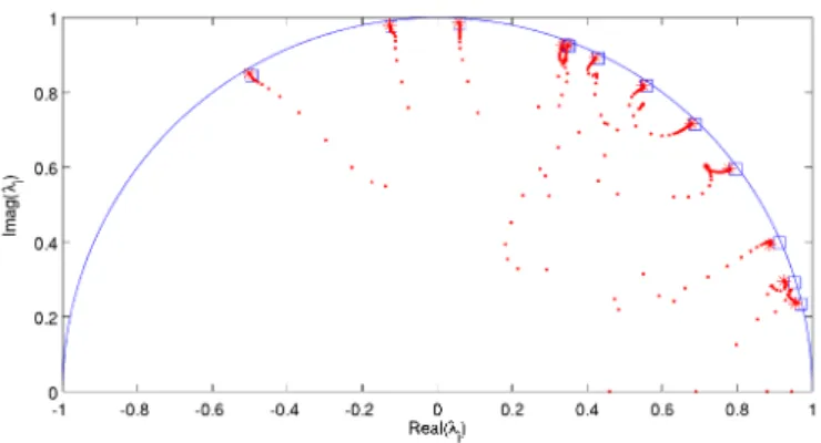
Figure 3. Theoretical eigenvalues (2) and eigenvalues of matrix A identified using EM (∗). The points represent the evolution of the eigenvalues of matrix A with respect to the iterations.
the number of modes). The corresponding values of the standard deviation error (std) are shown in this table too.
Furthermore it is presented in detail the results obtained with one of these 100 time history responses. The eigenvalues of the matrixA∈R24×24 identified using the proposed identification
method has been plotted in Fig. 3 together with theoretical eigenvalues. This figure shows a good estimation of the 12 eigenvalues. The evolution with the iterations from the starting values to the final EM parameters are also shown in that figure.
7 CONCLUSIONS
The first aim of this paper was to present a time-domain stochastic system identification method based on Maximum Likelihood Estimation and Expectation Maximization algo-rithm. The effectiveness of the proposed method has been evaluated through a numerical simulation study in the context of the ASCE benchmark problem. The numerical results show that the proposed method identifies eigenfrequencies, damping ratios and mode shapes reasonably well in the presence of 30% measurement noises even. In this simulated analysis, where the estimates can be compared with the exact solution, the proposed method has proved to be precise.
Advantages of the proposed structural identification method can be summarized as follows:
1. The method is based on maximum likelihood, that implies minimum variance estimates;
2. EM is a computational simpler estimation procedure than other optimization algorithms;
3. The method estimate all the parameters, and this estimates are accurate.
On the contrary, the main disadvantage of the method is the time needed until convergence is reached: first, because the EM algorithm is an iterative procedure, and second, because the initial point is located by means of a Montecarlo procedure.
ACKNOWLEDGMENTS
Figure 2. Identified natural frequencies of the full set of 100 simulations (•). The exact values of the frequencies are also plotted (continuous line).
frequency (Hz) damping ratio (%) mode shape (mac)
mode exact mean std exact mean std mean std n
1 9.41 9.75 8.82 1.00 8.75 0.85 0.775 25.55 89
2 11.79 12.26 23.12 1.00 10.57 1.00 0.969 8.05 96
3 16.38 16.46 26.92 1.00 4.70 0.55 0.994 0.72 100
4 25.54 25.76 12.58 1.00 1.70 0.51 0.505 20.71 97
5 32.01 32.27 7.98 1.00 1.36 0.33 0.920 2.54 100
6 38.66 38.83 4.10 1.00 1.10 0.30 0.892 15.50 96
7 44.64 45.16 2.81 1.00 1.14 0.27 0.895 0.93 100
8 48.01 48.35 19.77 1.00 1.09 0.38 0.279 13.60 100
9 48.44 48.55 21.78 1.00 1.15 0.27 0.822 6.85 100
10 60.15 60.46 4.94 1.00 0.87 0.13 0.934 1.62 100
11 67.48 67.71 4.29 1.00 0.87 0.16 0.993 0.30 100
12 83.62 83.69 6.58 1.00 0.47 0.01 0.975 1.32 100
Table 1. Resulting modal parameters for EM method. std is the standard deviation error (×10−2) and n is the number of simulations
where the parameters have been identified.
REFERENCES
[1] E. A. Johnson, H. F. Lam, L. S. Katafygiotis, J. L. Beck., Phase I IASC - ASCE structural health monitoring benchmark problem using simulated data, Journal of Engineering Mechanics, 130(1), 315. 2004.
[2] Jer-Nan Juang,Applied System IdentificationPrentice Hall PTR. 1994. [3] R.H. Shumway and D.S. Stoffer,Time series analysis and its applications,
Springer, 2006.
[4] M. Verhaegen, V. Verdult, Filtering and System Identification. A least squares approachCambridge University Press. 2007.
[5] F.J. Cara et all, Maximum likelihood estimation of modal parameters in structures using the Expectation Maximization algorithm, Proceedings of the Tenth International Conference on Computational Structures Technology, Civil-Comp Press, 2010.