Phoneme and Sub-Phoneme T-Normalization for Text-Dependent Speaker Recognition

Phoneme and Sub-Phoneme T-Normalization for

Text-Dependent Speaker Recognition

Doroteo T. Toledano

1

, Cristina Esteve-Elizalde

1

, Joaquin Gonzalez-Rodriguez

1

,

Ruben Fernandez Pozo

2

and Luis Hernandez Gomez

2

.

1

ATVS Biometric Recognition Group, Universidad Autonoma de Madrid, Spain

{doroteo.torre, cristina.esteve, joaquin.gonzalez}@uam.es

2

GAPS, SSR, Universidad Politecnica de Madrid, Spain

{ruben, luis}@gaps.ssr.upm.es

Abstract

1

Test normalization (T-Norm) is a score normalization technique that is regularly and successfully applied in the context of text-independent speaker recognition. It is less frequently applied, however, to dependent or text-prompted speaker recognition, mainly because its improvement in this context is more modest. In this paper we present a novel way to improve the performance of T-Norm for text-dependent systems. It consists in applying score T-Normalization at the phoneme or sub-phoneme level instead of at the sentence level. Experiments on the YOHO corpus show that, while using standard sentence-level T-Norm does not improve equal error rate (EER), phoneme and sub-phoneme level T-Norm produce a relative EER reduction of 18.9% and 20.1% respectively on a state-of-the-art HMM based text-dependent speaker recognition system. Results are even better for working points with low false acceptance rates.

1.

Introduction

Automatic Speaker Recognition (SR) aims to recognize the speaker that produces a particular speech utterance. Depending on the constraints imposed on the linguistic content of the utterance, there is text-independent speaker recognition, in which the linguistic content of the speech recording is unknown by the system, and text-dependent speaker recognition, in which the linguistic content of the speech is known by the system. In the latter case the text could be a password set by the user during training or a random text that is generated by the system and prompted to the user (text-prompted). A combination of both systems (first requesting a user-defined password and then a system generated prompt) provides increased security in voice authentication.

Despite its potential applications in interactive voice response systems, text-dependent SR has developed at a slower pace than text-independent SR. One of the reasons for this difference is the absence of competitive evaluation campaigns (such as the text-independent SR evaluations organized almost yearly by NIST [1,2]). Other reason is the lack of challenging benchmarks. For years YOHO [3, 4] has been the better known database for evaluation of text-dependent SR.

1

This work was funded by the Spanish Ministry of Science and Technology under project TEC2006-13170-C02-01.

In the field of text-dependent SR there are two methods that have been used for years: Dynamic Time Warping (DTW) and Hidden Markov Models (HMMs). DTW is simpler, but less flexible. For instance it is difficult, though not impossible [5], to build a text-prompted system with DTW. HMMs on the other hand may be a bit more complex, but provide greater flexibility and at least comparable results. Perhaps for this reason it is the most commonly used technique in text-dependent SR. Among the first researchers that advocate for the use of HMMs for text-dependent SR we should mention Matsui and Furui [6]. Later Genoud et al. proposed the combination of HMMs and DTW for improved performance [7]. Different configuration parameters in HMM based text-dependent SR were extensively tested within the context of the CAVE project [8]. The information from the alignment was proposed as an additional discriminative feature in [9]. More recently, the HMM framework has been combined with boosting [10] for improved performance.

In this paper we focus on text-dependent SR using HMMs, and in particular on the application of T-Norm score normalization. The use of T-Norm for text-dependent SR has received little attention until very recently [11, 12]. Of particular interest for this paper is the work in [12], where the authors propose the effect of the lexical mismatch as one of the reasons for the modest performance of T-Norm in text-dependent SR. In [12] the authors propose a technique for smoothing the normalization that improves the results. Here we present an alternative way of improving the performance of normalization, by performing T-Norm at the phoneme or sub-phoneme levels instead of at the utterance level.

The rest of the paper is organized as follows: section 2 describes the baseline algorithm used for text-dependent SR with HMMs. Section 3 describes the three different alternatives considered for performing T-Norm, and section 4 presents experimental results. Finally, section 5 presents some conclusions.

2.

General framework for text-dependent SR

based on phonetic HMMs

The general framework used in this paper for text-dependent SR is defined by a common parameterization; a speaker-dependent sentence HMM of the utterance to be verified (λ

D),

constructed from its phonetic transcription by concatenating a set of corresponding speaker-dependent phoneme models; a speaker-independent sentence HMM (λ

same way and used for log-likelihood score normalization; and a common way of scoring with all this information.

2.1. Parameterization

All the systems presented in this paper use a common signal processing front-end. After pre-emphasis, the signal is windowed using 25 ms. Hamming windows with a window shift of 10 ms. From each window 13 Mel Frequency Cepstral Coefficients (MFCCs) are extracted (including C0), and their first and second-order differences are calculated, for a total of 39 features per frame. We will represent the parameterized utterance as O={o1,o2,...,oN}, where N is the number of frames.

2.2. Speaker-independent HMM, λ

I

For each utterance we wish to verify we need to construct a speaker-independent HMM. To allow for total flexibility in the selection of utterances, we have trained 39 English context-independent phonetic HMM models on the TIMIT corpus [15]. Each phonetic model has the same topology (3 states, left-to-right with no skips). We have trained models with different complexities (1 to 80 Gaussians/state) to analyze the influence of this parameter. The phonetic models are combined into word models using a phonetic lexicon and the word models into an utterance HMM model via a grammar that allows only one sequence of words (the expected text in the utterance) with optional silences between them. We refer to this composite sentence HMM as λ_{I to denote that it is a} speaker-independent model of the utterance.

2.3. Speaker-dependent HMM, λ_D

For each utterance to be verified we need to construct a speaker-dependent sentence HMM. This sentence HMM is composed of speaker-dependent context-independent phonetic HMMs obtained from a small amount of speech (enrollment data) from that speaker. These speaker-dependent phonetic HMMs are structurally equivalent to the speaker-independent HMMs – they have the same topology and same number of Gaussians per state. There are different ways to obtain speaker-dependent HMMs. We have explored two of them: performing Baum-Welch reestimation [13] of the speaker-independent phonetic HMMs on the enrollment data, and adapting the speaker-independent HMMs using Maximum Likelihood Linear Regression (MLLR) [14]. The last option yields better results for limited amounts of enrolment data and has the additional advantage that only the MLLR adaptation matrices need to be stored as the speaker model, which represents a considerable amount of storage saving. These speaker-dependent phonetic models are combined into a sentence HMM model in exactly the same way as with the independent ones. We represent the speaker-dependent sentence HMM as λ

D.

2.4. Scoring

Given a test sentence (of which we know the text) and a speaker model, scoring proceeds as follows. We first parameterize the sentence obtaining a sequence of feature vectors, O={o1,o2,...,oN}. We then construct a speaker-independent sentence HMM model (λ

I) and a

speaker-dependent sentence model (λ_D). Two different state

segmentations are obtained through Viterbi decoding from both the speaker independent model, λ_{I, and the speaker} dependent model, λ_{D. This decoding is almost a forced} phonetic alignment (the only exceptions are the optional silences) because no alternative pronunciations are considered. At this stage, given the set of observations O these two Viterbi alignments produce the following information:

(i) The best state per frame given O and λ

I or λD:

{

( | , )

}

max arg } ,..., ,

{1 2 I

I N I I

I s s s P

S _{Q O}λ

Q = = (1)

{

( | , )

}

max arg } ,..., ,

{1 2 D

D N D D

D s s s P

S Q O λ

Q =

= , (2)

where Q={q1,q2,...,qN}represents any possible state sequence.

This information can also be represented as a sequence of state labels (possibly spanning several frames) and a state segmentation } ,..., , { }, ,..., ,

{ 1 2 1 2

D L D D D I L I I

I sl sl sl I SL sl sl sl D

SL = = (3)

} ,..., , { }, ,..., ,

{ ₀I ₁I I_{L D 0}D ₁D _LD

I st st st I SS st st st D

SS = = , (4)

whereL_IandL_Dare the total number of decoded states for the

speaker independent and dependent models, sl_iX are the

labels of the states and st_iX the number of the frame at which

state sliX ends plus one ( X st0 is 0).

From these state sequences we can obtain the corresponding phoneme labelings and segmentations

} ,..., , { }, ,..., ,

{ ₁I ₂I _KI _{D 1}D ₂D _KD

I pl pl pl I PL pl pl pl D

PL = = (5)

} ,..., , { }, ,..., ,

{ 0 1 0 1

D K D D D I K I I

I pt pt pt I PS pt pt pt D

PS = = , (6)

whereKIand KDare the number of phonemes and silences

found with the speaker independent and dependent models,

X i

pl represents the phone and silence labels and X i pt is the

ending frame number of phoneme X i

pl plus one (_ptX

0 is 0).

(ii) The acoustic scores per frame (considering the best state sequence only) for the speaker independent and speaker dependent models:

(

)

     >       = = − 1 ) ( log 1 ) ( log 1 i b a i b acs i I s I s s i I s I s I i I i I i I i I i I i o o π (7)

(

)

     >       = = − 1 ) ( log 1 ) ( log 1 i b a i b acs i D s D s s i D s D s D i D i D i D i D i D i o o π

, (8)

where X

siX

π represents the initial state probabilities of the

HMMs (normally only one of these probabilities is 1 and the rest are 0), X

s siX iX a

1

−

represents the transition probabilities from

state s_iX₋₁to state s_iXin the HMMs and D ( _i)

s_iD

b o represents the

probability of observing o_iin state X i

s , according to the

With all this information at hand it is relatively straightforward to produce scores measuring the similarity of the sequence of feature vectors to be verified and the speaker model, λ_{D. The simplest measure may be the normalised} log-likelihood score obtained from the difference between the average acoustic score per frame for the utterance, given the speaker dependent model (λ_D), and the average acoustic score from the speaker-independent (λ_{I) model:}

        − =

∑

∑

= = N i I i N i D i

D acs acs

N sc 1 1 1 1 ) ,

(Oλ . (9)

The possible contribution of initial, final and inter-word silences to the score in eq. (9) carries no information that is valuable for speaker discrimination. Consequently, to improve its discriminative capabilities silence frames should be excluded from the score. Thus we obtain:

∑ ∑

∑ ∑

∉ = − = ∉ = − = _{− −} − = I I i I i I i D D i D i D i K SIL pl i pt pt j I j I K SIL pl i pt pt j D j D D acs N acs N sc 1 1 * 1 1 * 2 1 1 1 1 ) ,

(_Oλ _{, (10)}

Where SIL is the set of silence labels and *

D

N and *

I N are the number of non-silence frames found in the Viterbi with the speaker-dependent model and speaker-independent model, respectively.

In spite of the score normalization provided by the use of speaker-independent scores, which can be viewed as similar to a UBM (Universal Background Model) and cohort-normalisation, the speaker-dependent score variation and the need for speaker-independent decision thresholds usually requires the inclusion of further score normalization techniques (Z-norm, T-norm, …). In this sense we can describe Eq. (10) as defining the scoring mechanism employed to compute the unnormalized scores in our text-dependent speaker verification system.

3.

T-Norm for text-dependent SR at the

utterance, phoneme and state levels

In text-independent SR it is very common to use T-Normalization by comparing the score obtained with a test segment, not only to the model of the speaker in the test segment, but also against the models of other speakers (i.e. against a cohort of impostors).

3.1. Utterance-level T-Norm

The direct translation of this approach to text-dependent SR is what we call utterance-level T-Norm, to distinguish it from the novel T-Normalization schemes proposed in following sections. In utterance-level T-Norm for text-dependent SR we need to create a cohort of M speaker sentence HMM models for the utterance, { 1, 2,..., M}

D D D O

C ₌ λ λ λ . This set of sentence HMMs needs to be created from the textual content of each test utterance using the speaker-dependent phonetic HMMs of each of the speakers in the cohort, as explained in sections 2.2 and 2.3.

Once these models are in place we can use eq. (10) to compute the score of the test utterance against each speaker in the cohort,{ ( , ), ( , 2),..., ₂( , )}

2 1 2 M D D

D sc sc

sc Oλ O λ O λ , compute

the mean, O C

µ , and the standard deviation, O C

σ , of these scores and T-Normalize the score as usual,

O C O C D D TNorm sc sc σ µ − = ( , ) ) , ( 2 2 λ O λ

O . (11)

3.2. Phoneme-level T-Norm

One problem with the utterance-level T-Norm scheme applied to text-dependent SR is that we are trying to normalize an average score computed on parts of the test utterance that can be very different (for instance computed on different phonemes). For that reason it makes sense to try to normalize the scores for similar segments before averaging the scores.

To achieve this goal, we first realize that the sequence of phonemes (excluding silences) produced by the Viterbi decodings is the same for all the models (λD,

M D D D λ λ

λ1 _, 2_{,..., ,} and λI), as discussed in sections 2.2 and 2.3. Let us define

this common sequence of phonemes as

} ,..., ,

{ 1 2

All K All All

All pl pl pl

PL = . We can now find mapping

functions that map the indices 1, … , K into the index corresponding to the same phoneme in each of the Viterbi

decodings. Let us call these mappings

) (i

m_D ,m1_D(i),m2_D(i),...,m_DM(i), and m_I(i). With these mappings we propose to approximate Eq. (10) as

        = ≈

∑

= K i D p D p

D N isc i

N sc sc 1 * *

2 () ( , ,)

1 ) , ( ) ,

(_Oλ _Oλ _Oλ _{, (12)}

whereN*is the average number of non-silence frames found with the speaker-dependent and speaker-independent models,

2 / )] ( ) [( )

( () ()1 () ()1

* I i m I i m D i m D i

mD pt D pt I pt I

pt i

N = − − + − − , (13)

is the average number of frames found for phoneme All i pl in the speaker dependent and speaker independent decodings, and

∑

∑

− = − − = − − − − − − = 1 1 ) ( ) ( 1 1 ) ( ) ( ) ( 1 ) ( ) ( 1 ) ( ) ( 1 ) ( 1 ) , , ( I i I m I i I m I I D i D m D i D m D D pt pt j I j I i m I i m pt pt j D j D i m D i m D p acs pt pt acs pt pt i

sc _Oλ

, (14)

is the speaker recognition score produced only by phoneme

All i pl .

After this small transformation we can compute the scores for each of the phonemes (i) in PL_All against the speaker

model,sc_p(_O,λ_D,i)_{, and also against each of the T-Norm}

cohort models,scp(O,λ1D,i),...,scp(O,λMD,i). Now we can compute a T-Normalized score for each of the phonemes in

All

PL , scTNorm_p (_O,λ_D,i)_{, and then combine the T-Normalized} phonetic scores as in eq. (12).

prior to compute the global average, which should lead finally to a better score normalization.

3.3. State-level T-Norm

As shown in section 2.4, Viterbi decodings produce a phoneme labelling and segmentation and also a more detailed HMM state labelling and segmentation. Following an argumentation parallel to that presented in section 3.2 we can define a speaker recognition score for each state found in the decoding that does not correspond to a silence, and also an approximation to eq. (10) very similar to eq. (12) to compute the overall score from those state-level scores. After having presented the phoneme-level T-Norm it is quite obvious that this idea can easily be extended to a state-level T-Norm

scheme in very much the same way as in section 3.2. With respect to the lexical content of the utterances state-level Norm has no theoretical advantage over phoneme-level T-Norm. However, the main reason to introduce more than one state in an HMM is co-articulation (the initial part of the phoneme is very much affected by the preceding phoneme and the final part by the following phoneme). Therefore, performing state-level T-Norm is a way of more finely treating co-articulation in T-Norm, and theoretically there are reasons to consider it better than phoneme-level T-Norm.

4.

YOHO experimental protocol

For the experiments we have used YOHO [3], probably the most widely used and well known benchmark for system comparison and assessment. It consists of 96 utterances for enrolment collected in 4 different sessions and 40 utterances for testing collected in 10 sessions for each of a total of 138 speakers, 106 male and 32 female. Each utterance is a different set of three digit pairs (e.g. “12-34-56”). The results presented on YOHO are based on the following experimental protocol. Speaker models are trained using 6 utterances from session 1, the 24 utterances from session 1 or the 96 utterances from the 4 sessions. Our main focus was on the single session, 6 utterances, since it is the closest to what we expect to find in realistic operational conditions. Speaker verification is performed using a single utterance from the test subset. The target scores are generated by matching each speaker-dependent phone HMM with all the test utterances from that user, leading to a total of 138 x 40 = 5,520 scores. The impostor scores are computed by comparing each speaker model with a single utterance randomly selected from those of all other users, which yields 138 x 137 = 18,906 trials. For all impostor trials the sentence HMMs are produced using the actual text spoken to simulate a text-prompted system in which the impostors know what they have to say.

For experiments using T-Norm the experimental protocol has been slightly modified. In particular, we have reserved 10 male and 10 female speakers to build a 20-speaker cohort for T-Normalization. This way the number of target scores is reduced to 118 x 40 = 4,720, and the number of impostor scores to 118 x 117 = 13,806.

5.

Results

We have organized this section into two subsections. The first one compares results without score normalization using MLLR and Baum-Welch to obtain the speaker model. The

second focuses on the three different ways of performing T-Normalization that we have proposed above.

5.1. Results with MLLR and retraining

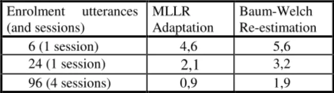
In this section we compare MLLR adaptation and Baum-Welch re-estimation for different amounts of enrolment speech. In particular, we have compared the best results achieved by MLLR adaptation and Baum-Welch retraining for the condition of 6 utterances from the first training session, 24 utterances from the first training session, and of all 96 utterances in the 4 training sessions. Table 1 and Figure 1 show the best results obtained after an optimization performed on the number of Gaussians per state, the number of iterations of Baum-Welch re-estimation and the number of regression classes in MLLR adaptation. For Baum-Welch re-estimation the number of Gaussians per state was varied between 1 and 5 and the number of re-estimation iterations was either 1 or 4. For MLLR adaptation the number of Gaussians per state was varied between 5 and 80 in steps of 5 and the number of regression classes between 1 and 32 in power-of-2 steps. Our best results show that, even in the cases with the largest amount of data, MLLR adaptation outperforms Baum-Welch re-estimation in text-dependent speaker recognition. In fact, the difference in favour of MLLR tends to increase as the amount of enrolment material increases. The reason for this may be that the amount of enrolment material, even using the 96 utterances for training, is still very limited for Baum-Welch re-estimation. MLLR adaptation seems to be more adequate for the whole range of enrolment speech considered.

Figure 1: DET curves obtained on YOHO with MLLR adaptation and Baum-Welch re-estimation, using as enrolment material 6, 24 and 96 utterances.

Table 1. EERs (%) obtained on YOHO with MLLR adaptation and Baum-Welch re-estimation, using as enrolment material 6, 24 and 96 utterances.

Enrolment utterances (and sessions)

MLLR Adaptation

Baum-Welch Re-estimation

6 (1 session) 4,6 5,6

24 (1 session) _2,1 3,2

5.2. Results with utterance, phoneme and state-level T-Norm

In the work we describe in this section we have focused on the speaker-dependent models that produced the best results in the former section, the MLLR adapted models, and on user enrolment with 6 utterances, which we consider the most realistic case. With these settings we have tested the different schemes for T-Normalization described in section 3.

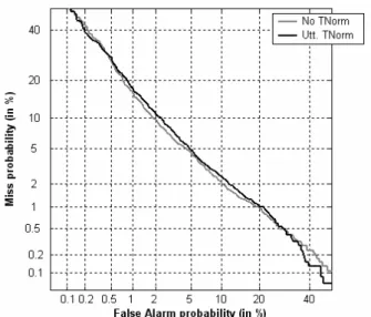
Figure 2 compares the results obtained by not using T-Norm with those obtained using utterance-level T-Norm (i.e. the usual way in which T-Norm is applied in text-independent SR). Results not using T-Norm are equivalent to those presented in Figure 1 and Table 1. There are, however, small differences due to the slightly different experimental protocol (we set aside 20 speakers as our T-Norm cohort). Results with

utterance-level T-Norm are slightly worse for most of the DET curve. This unexpected worsening could be due primarily to the small cohorts used. Regarding this factor, we were very limited by YOHO because we only have 36 female speakers and we couldn’t set aside more speakers for the cohort. We tried, however, to perform T-Normalization with 4 models per speaker, trained on the first 6 sentences of each training session for each speaker. Results using this utterance-level T-Norm with a cohort of 80 models (from 20 speakers) are presented in Figure 3. In this case, results with T-Norm are slightly better than results without T-Norm, but the overall improvement achieved with T-Norm probably does not justify the increase in computational cost.

Figure 4 compares the results obtained by not using T-Norm with those using phoneme-level T-Norm with a cohort of 20 speaker models (i.e. same condition as Figure 2). Results show noticeable improvements when using phoneme-level T-Norm. Results not using T-Norm in Figure 4 are obtained with the approximation given by eq. (12). This explains the small differences between the DET curve for no T-Norm in Figures 2 and 4.

Figure 2: DET curves with and without T-Norm (at the utterance level). Results obtained on YOHO (with only 6 utterances from a single session as enrollment material) using MLLR adaptation.

Figure 3: DET curves with and without T-Norm (at the utterance level) with 4 models per speaker in the cohort. Results obtained on YOHO (with only 6 utterances from a single session as enrollment material) using MLLR adaptation.

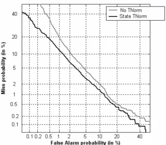
Finally, Figure 5 compares the results obtained by not using T-Norm with those using state-level T-Norm with a cohort of 20 speaker models (i.e. same condition as in Figures 2 and 4). These results show even greater improvements than those achieved using phoneme-level T-Norm. Again, results not using T-Norm in Figure 5 are obtained with an approximation for states similar to that of eq. (12). For this reason this curve is again different to the corresponding curves in Figures 2 and 4.

Table 2 summarizes the results achieved. For each type of T-Norm tested we present the Equal Error Rate and the relative improvement over the baseline (No T-Norm). Since the effect of T-Norm tends to be more evident in the area of low false acceptances, we also present in the table the False Rejection rate for a False Acceptance of 1% (FR@FA=1%). For the No T-Norm condition we have chosen the results shown in Figure 2 (i.e. those obtained applying eq. (10)). Results for the approximations in Figures 4 and 5 are worse in terms of the FR@FA=1% and similar in terms of EER.

Figure 5: DET curves with and without T-Norm (at the state level). Results obtained on YOHO (with only 6 utterances from a single session as enrollment material) using MLLR adaptation.

Table 2 shows clearly that utterance-based T-Norm is not working properly for this text-dependent task, producing drops in performance levels, probably due to lexical mismatch. Phoneme-based and state-based T-Norm produce relative improvements of nearly 20% in terms of EER and over 25% in terms of FR@FA=1%. These results show that both phoneme-level and state-level T-Norm are superior to the standard (utterance-level) T-Norm. State-level T-Norm is slightly better than phoneme-level T-Norm, probably due to its ability to normalize scores taking into greater account the effect of coarticulation.

6.

Conclusions

We have proposed and evaluated two new different methods to apply T-Norm in the context of text-dependent speaker recognition. T-Norm is regularly applied in text-independent speaker recognition. However, in text-dependent speaker recognition the T-Norm does not perform as expected, perhaps due to the problem of the lexical mismatch. We have proposed applying T-Norm at the phoneme level and also at sub-phoneme level (in particular at the level of HMM states). These methods provide different score normalization values (means and standard deviations) for different segmental units and, as we have shown empirically, they produce much better results than utterance-level T-Norm in a text-dependent speaker recognition task (YOHO).

7.

References

[1] “National institute of standard and technology. Speaker

Recognition Evaluation Home Page”,

http://www.nist.gov/speech/tests/spk/index.htm.

[2] M. A. Przybocki, A. F. Martin, and A. N. Le. “NIST speaker recognition evaluation chronicles part 2”, in

Proc. IEEE Odyssey 2006: The speaker and language recognition workshop.

[3] J. Campbell and A. Higgins. Yoho speaker verification (ldc94s16). http://www.ldc.upenn.edu.

Table 2. EERs and False Rejection (FR) rate at a False Acceptance (FA) rate of 1% obtained on YOHO (with only 6 utterances from a single session as enrollment material) using MLLR adaptation and different types of T-Norm. Relative improvements over the baseline (no T-Norm) are given in parentheses.

Type of T-Norm EER (%) (Rel. Improv. %)

FR@FA=1% (%) (Rel. Improv. %)

No T-Norm 4.82%

(0.0%)

16.28% (0.0%)

Utterance-based 5.01%

(-3.9%)

17.45% (-7.2%)

Phoneme-based 3.91%

(18.9%)

12.17% (25.2%)

State-based 3.85%

(20.1%)

11.81% (27.5%)

[4] J. P. Campbell, “Testing with the YOHO CD-ROM voice verification corpus”, in Proc. ICASSP 1995, vol. 1, pp. 341-344.

[5] V. Ramasubramanian, A. Das and V. P. Kumar, “Text-dependent speaker recognition using one-pass dynamic programming algorithm”, in Proc. ICASSP 2006, vol. 1, pp. 901-904.

[6] T. Matsui and S. Furui, “Speaker Recognition Using Concatenated Phoneme HMMs,” Proc. Int. Conf. Spoken Language Processing, Banfl, Th.sA M.4.3 (1992). [7] D. Genoud, F. Bimbot, G. Gravier and G. Chollet,

“Combining methods to improve speaker verification decision”, in Proc. ICSLP 1996, vol. 3, pp. 1756-1759. [8] F. Bimbot, H. P. Hutter, C. Jaboulet, J. Koolwaaij, J.

Lindberg and J. B. Pierrot, “Speaker verification in the telephone network: research activities in the CAVE project”, in Proc. Eurospeech 1997, pp. 971-974. [9] D. Charlet, D. Jouvet and O. Collin, “An alternative

normalization scheme in HMM-based text-dependent speaker verification”, in Speech Communication, vol. 31, issue 2-3, June 2000,,pp. 113-120.

[10]Subramanya, A.; Zhengyou Zhang; Surendran, A.C.; Nguyen, P.; Narasimhan, M.; Acero, A.; “A Generative-Discriminative Framework using Ensemble Methods for Text-Dependent Speaker Verification” in IEEE International Conference on Acoustics, Speech and Signal Processing (ICASSP), 2007. Volume 4, 15-20 April 2007 pp. IV-225 - IV-228. [11]R. D. Zilca, J. W. Pelecanos, U. V. Chaudhari, and G. N. Ramaswamy, “Real time robust speech detection for text-independent speaker recognition”, in Proc. IEEE Odyssey Speaker Recognition Workshop, 2004.

[12]M. Hébert and D. Boies, “T-Norm for text-dependent commercial speaker verification applications: effect of lexical mismatch”, in Proc. ICASSP 2005, pp. 729-732. [13]L. R. Rabiner, “A Tutorial on Hidden Markov Models”,

In Proceedings of the IEEE, vol. 77, n. 2, February 1989, pp. 257-286.