Abstract—Goal: The purpose of this study is to evaluate the usefulness of the boosting algorithm AdaBoost (AB) in the context of the sleep apnea-hypopnea syndrome (SAHS) diagnosis. Methods: We characterize SAHS in single-channel airflow (AF) signals from 317 subjects by the extraction of spectral and non-linear features. Relevancy and redundancy analyses are conducted through the fast correlation-based filter (FCBF) to derive the optimum set of features among them. These are used to feed classifiers based on linear discriminant analysis (LDA) and classification and regression trees (CART). LDA and CART models are sequentially obtained through AB, which combines their performances to reach higher diagnostic ability than each of them separately. Results: Our AB-LDA and AB-CART approaches showed high diagnostic performance when determining SAHS and its severity. The assessment of different apnea-hypopnea index cutoffs using an independent test set derived into high accuracy: 86.5% (5 events/h), 86.5% (10 events/h), 81.0% (15 events/h), and 83.3% (30 events/h). These results widely outperformed those from logistic regression and a conventional event-detection algorithm applied to the same database. Conclusion: Our results suggest that AB applied to data from single-channel AF can be useful to determine SAHS and its severity. Significance: SAHS detection might be simplified through the only use of single-channel AF data.
Index Terms—AdaBoost, airflow, sleep apnea-hypopnea syndrome, spectral analysis, nonlinear analysis
I. INTRODUCTION
n recent years, the Sleep Apnea-Hypopnea Syndrome (SAHS) has become a major concern due to the high prevalence and severe consequences for the patients’ health and quality of life [1], [2]. People suffering from SAHS experiment recurrent episodes of complete (apnea) or partial (hypopnea) collapse of the upper airway during sleep, which
*This research was supported by the Proyecto Cero 2011 on Ageing from
Fundación General CSIC, the project TEC2011-22987 from Ministerio de Economía y Competitividad, the project VA059U13 from the Consejería de Educación de la Junta de Castilla y León, and FEDER. G. C. Gutiérrez-Tobal was in receipt of a PIRTU grant from the Consejería de Educación de la Junta de Castilla y León and the European Social Fund.
G. C. Gutiérrez-Tobal, D. Álvarez, and R. Hornero, are with the Biomedical Engineering Group of the University of Valladolid, Spain (corresponding author e-mail: [email protected])
F. del Campo is with the sleep unit of Hospital Universitario Rio Hortega in Valladolid, Spain (e-mail: [email protected]).
lead to cessation or significant reduction of airflow (AF) [3]. These apneic events cause oxygen desaturations and arousals [3], preventing patients from resting while sleeping [2]. Unsuccessful rest derives in daytime symptoms such as hypersomnolence, cognitive impairment, and depression [1], some of which have been related to motor-vehicle collisions and occupational accidents [4], [5]. Moreover, SAHS has been associated with cardiac and vascular illnesses [2], as well as with an increase in the cancer incidence [6].
The standard test to diagnose SAHS is overnight in-lab polysomnography (PSG) [3]. Although its effectiveness is well-known, PSG implies monitoring and recording multiple physiological signals, including electrocardiogram (ECG), electroencephalogram (EEG), electromyogram (EMG), oxygen saturation of blood (SpO2), and AF [3]. This makes
PSG a complex test which requires expensive equipment and technical expertise [7], [8]. Moreover, the specialists need an offline inspection of the recordings to derive the apnea-hypopnea index (AHI), which is the parameter used to establish SAHS and its severity [9]. Thus PSG is also time-consuming, leading to a delayed diagnostic process and increased waiting lists [8], [10].
One widespread approach to reduce complexity, cost, and time delay is the study of a limited set of signals among those involved in PSG [8]. The analysis of a single one has been often adopted. Thus, the oxygen desaturation index (ODI) from SpO2, the apneic-related events from ECG, and the
respiratory disturbance index (RDI) from AF have been already assessed to help in SAHS diagnosis [10]-[13]. These works followed a common methodology: detecting the effects caused by each apnea and hypopnea in the signals under study, scoring them as apneic-related events, and deriving the corresponding diagnostic index. However, our research group has lately adopted a different approach based on an exhaustive analysis of a signal through the extraction of global features [14]-[18].
In this paper, we propose such a global analysis in single-channel AF. AF is a straightforward choice to look for simpler alternatives to PSG, since apneas and hypopneas are defined on the basis of its amplitude oscillations [9]. The American Academy of Sleep Medicine (AASM) recommends the use of two AF channels: one acquired through an oronasal thermal sensor and the second one acquired by means of a nasal prong
Gonzalo C. Gutiérrez-Tobal
*,
Student Member
,
IEEE
, Daniel Álvarez,
Member, IEEE,
Félix del
Campo, and Roberto Hornero,
Senior Member
,
IEEE
Utility of AdaBoost to Detect Sleep
Apnea-Hypopnea Syndrome from Single-Channel
Airflow
pressure sensor (NPP) [9]. The former is suitable for a proper scoring of apneas whereas the latter is used to score hypopneas [9]. However, previous studies have shown that it is possible to reach high diagnostic ability following an automatic global analysis of the single-channel AF from a thermal sensor [17], [18]. In this paper, one major goal is to assess whether it is also possible to reach a high performance when using data from single-channel AF obtained by NPP.
Our proposal starts with the extraction of spectral (frequency domain) and non-linear (time domain) features from NPP AF. The analysis in frequency domain is justified due to the overnight recurrence of these events. Thereby, common spectral features have already shown their utility to characterize SAHS as well as other disorders [15]-[19]. On the other hand, non-linear measures of variability, complexity, and irregularity in time series have been also used to extract useful information from biomedical signals [14], [17]-[19]. This exhaustive characterization of AF, however, may lead to obtain features with a high degree of shared information, i.e., redundant features. In order to avoid this issue, a second step is included in our methodology: an automatic feature selection stage based on the fast correlation-based filter (FCBF) [20]. The FCBF algorithm selects optimum sets of features on the basis of their relevancy and redundancy. It has been also assessed in biomedical applications [17], [21]. Finally, a classification approach is used to distinguish SAHS and its severity. Thus, we evaluate two different cases: a binary classification task, in which the objective is to determine the presence (SAHS-positive) or absence (SAHS-negative) of SAHS, and a multiclass task, in which the aim is to assess the AHI cutoffs which establish the four severity levels of SAHS (no-SAHS, mild-SAHS, moderate-SAHS, and severe-SAHS). We propose the AdaBoost (AB) algorithm for both classification tasks. AB is a boosting algorithm commonly used to take advantage of the performance of several weak classifiers of the same type [22]. It is known to be able to reach high yields when it is applied to new data [22], i.e., the AB algorithm produces generalized models. Moreover, it relies on a simple sequential procedure [22], which barely increases the complexity of the methodology. These characteristics make it a suitable algorithm to be used in diagnostic aid contexts. Actually, it has been already assessed in the context of SAHS under a classic event-detection approach [23], [24]. As weak classifiers we propose two well-known machine learning algorithms based on i) linear discriminant analysis (LDA) and ii) classification and regression trees (CART). Both of them have been already assessed in the context of SAHS [16], [23]. Since classifiers favor the right sorting of classes with more subjects, one major issue in the present work is how to deal with imbalanced classes. The high prevalence of SAHS leads to prioritize diagnosis in at-risk population [25]. Consequently, data from SAHS patients is more available than from no SAHS subjects. Thus, to compensate for this imbalance, we use the synthetic minority oversampling technique (SMOTE) [26], which creates new synthetic data from the minority classes on the basis of the real data.
Our hypothesis is that the information obtained from AF and the generalization ability of AB can be useful to automatically detect SAHS and establish its severity. Thus, the main objective of the present work is to evaluate the diagnostic usefulness of AB when the only source of SAHS-related information is single-channel AF from NPP. In order to achieve this goal, we evaluate whether our proposal outperforms the diagnostic ability of a typical classification algorithms such as logistic regression (LR), which is based on one single classifier. We also apply to our AF recordings an algorithm focused on the classical event-detection approach, which has been previously assessed in other databases [17], [27]. Finally, our results are also compared with other recent studies focused on SAHS detection from single-channel AF.
II. POPULATION AND SIGNAL UNDER STUDY
In this study, AF recordings from 317 adults were involved. Before undergoing PSG, all of the subjects suffered from common symptoms such as daytime sleepiness, loud snoring, nocturnal choking and awakenings, and/or referred apneic events. PSG was conducted in the sleep unit of the Hospital Universitario Río Hortega in Valladolid, Spain. Physicians scored apneas and hypopneas according to the American Academy of Sleep Medicine (AASM) rules [9]. Consequently, an apnea was defined as a 90% or more reduction in the pre-event baseline of the AF amplitude, measured through an oronasal thermal sensor. In contrast, a hypopnea was scored after 30% or more reduction in the pre-event baseline of the AF amplitude, measured through a nasal pressure sensor, and accompanied by a drop of 3% in SpO2 and/or an EEG arousal.
In both cases, duration of 10 seconds or more was required to annotate the event [9]. All the subjects gave their informed consent and the Ethics Committee of the Hospital Universitario Rio Hortega (Spain) accepted the protocol.
Common AHI cutoffs to determine SAHS and its severity are 5, 10, 15, and 30 e/h [9], [10], [13], [17]. Particularly, SAHS severity levels are: no-SAHS (5AHI), mild-SAHS (5≤AHI15), moderate-SAHS (15≤AHI30), and severe-SAHS (AHI30) [28]. Alternatively, AHI=10 e/h has been widely used as cutoff to determine the presence or absence of SAHS [10], [13], [17], [18], [29]. Consequently, for the binary classification task, we chose AHI=10 e/h to distinguish SAHS-negative and SAHS-positive subjects, whereas for the multi-classification task we divided our database according to the four SAHS severity levels. Tables I and II show clinical and demographical data of the subjects under study when they are divided for the binary or the multiclass tasks, respectively. No statistically significant differences were found (p-value0.01) between SAHS-positive and SAHS-negative (Mann-Whitney U test), or among the four severity levels (Kruskal-Wallis test), in body mass index (BMI) and age.
applied to the AF recordings to satisfy the Nyquist-Shannon theorem. We also applied an infinite impulse response Butterworth low-pass filter (cutoff = 1.2 Hz) to reduce noise for a prospective non-linear analysis in time domain.
We divided our recordings into a training set (60%) and a test set (40%). A uniformly random selection was conducted to assign the AF recordings to each one. However, for the sake of the balance of the classes in the training set, we fixed the size of each class as follows: 29 no-SAHS subjects, 54 mild-SAHS, 54 moderate-mild-SAHS, and 54 severe-SAHS. This distribution in the multiclass problem leads to 75 SAHS-negative and 116 SAHS-positive for the binary classification task. The SMOTE algorithm was used to compensate the remaining imbalance in classes of the training set (section F). The recordings not selected for the training set were assigned to the test set.
III. METHODS
Our methodology consists of three steps. First, a feature extraction stage is implemented, in which spectral and nonlinear analyses are conducted over the AF recordings. Then, an automatic feature selection is performed to obtain an optimum set of the extracted features. Finally, a boosting classification approach is adopted to determine SAHS (binary classification) and its severity (multiclass task). Fig. 1 depicts a block diagram with the entire methodology followed during the study, which is widely explained in next sections.
A. Feature extraction
1) Spectral analysis
Apneas and hypopneas recurrently modify AF throughout the night. This behavior supports its study in the frequency domain. Hence, the power spectral density (PSD) of each AF recording was estimated. Welch’s method was applied for this purpose since it is suitable for non-stationary signals [30]. A Hamming window of 215 points (50% overlap), along with a
discrete Fourier transform of 216 points, were used to compute
PSD. To avoid the influence of factors not related to the pathophysiology of SAHS, each PSD was normalized (PSDn) dividing the amplitude value at each frequency by their corresponding total power [31]. Fig. 2a shows the averaged
PSDn for the four SAHS severity groups in the training set. A spectral band of interest (BW) was defined between 0.025 Hz. and 0.050 Hz. (Fig. 2b). This corresponds to events lasting from 20 to 40 seconds, which has been reported as the typical range of the apneic events duration [32]. Moreover, BW is consistent with the bands found through statistical approaches [17], [18]. Thus, to characterize SAHS, 9 spectral features were extracted from the 0.025-0.050 Hz. band of each PSDn: minimum amplitude (mA), maximum amplitude (MA), first to fourth statistical moments (Mf1- Mf4), median frequency (MF),
spectral entropy (SpecEn), and Wootters distance (WD). mA and MA were computed as the lowest and the highest PSDn values in BW. Since PSD is normalized, the amplitude values of the original AF time-series do not affect the power at each frequency component. Hence, as BW is related to apneic events, mA and MA estimate the minimum and the maximum occurrence of them. Mean (Mf1), standard deviation (Mf2),
skewness (Mf3), and kurtosis (Mf4) of BW were also obtained.
They are common statistics which quantify central tendency, dispersion, asymmetry, and peakedness of data, respectively. According to Fig. 2b, mA and MA should be higher as SAHS worsens. Similarly, the mean (Mf1) and the standard deviation
(Mf2) should be also higher. Finally, both the skewness (Mf3)
and the peakedness (Mf4) seem to be higher in the BW spectral
data of moderate and severe groups.
MF is defined as the frequency component which separates the spectrum into two parts with 50% of the power each of them [33]. Thus, the lower the MF value, the more comprised is the spectrum into small frequencies. As seen in Fig 2b, the spectrum of BW for the no-SAHS and mild-SAHS groups is flat, i. e., the power is equally distributed. Conversely, a fewer
Fig. 1 Block diagram of the signal processing methodology followed during the study.
TABLE I
DEMOGRAPHIC AND CLINICAL DATA FOR THE TWO-CLASS DIVISION
All SAHS-negative SAHS-positive
# Subjects 317 110 207
Age (years) 49.9 12.0 47.6 12.9 51.1 11.4 Men (%) 226 (71.3) 68 (61.8) 158 (76.3) BMI (kg/m2) 28.1 5.2 26.5 5.0 29.0 5.1
AHI (e/h) 28.1 26.5 6.0 2.6 39.9 25.9
TABLE II
DEMOGRAPHIC AND CLINICAL DATA FOR THE FOUR-CLASS DIVISION
no-SAHS mild moderate severe
# Subjects 39 92 70 116
Age (years) 43.9 12.5 50.3 12.4 49.9 11.3 51.6 11.5 Men (%) 19 (48.7) 58 (63.0) 56 (80.0) 93 (80.2) BMI(kg/m2)
amount of power is observed in higher frequencies of BW for moderate-SAHS and severe-SAHS groups. As a consequence, a MF value closer to 0.0375 (the half of the band) is expected for the lowest severity degrees.
SpecEn quantifies the flatness of the PSD content, which
indirectly measures the irregularity of time series [33]. Thereby, high values of SpecEn are related to a flat PSD (similar to white noise) and, consequently, it is associated with more irregularity in time domain. By contrast, low values imply a spectrum condensed into a narrow frequency band, which is related to less irregularity in time domain (like in a sum of sinusoids) [33]. A flatter spectrum is observed in BW as SAHS severity decreases. Therefore, higher values of
SpecEn are expected in no-SAHS and mild-SAHS groups.
WD is a disequilibrium measure which assigns values close to 1 to those distributions with higher statistical distance to the uniform distribution; whereas values close to zero are assigned as the distance becomes smaller [34], [35]. In BW, the averaged spectrum of the no-SAHS and mild-SAHS groups is similar to a normal distribution (Fig. 2b). Hence, smaller values of WD are expected than in the case of the moderate-SAHS and severe-moderate-SAHS groups.
2) Non-linear analysis
Alterations caused by SAHS in AF could modify the variability, the complexity, and the irregularity of the signal. Hence, to complement the spectral analysis, three global non-linear features were also obtained from each recording in time domain: central tendency measure (CTM), Lempel-Ziv complexity (LZC), and sample entropy (SampEn). Similarly to
PSD, each AF time series was normalized before obtaining CTM, LZC, and SampEn. Thereby, measuring effects caused by factors not related to the pathophysiology of SAHS are avoided. We firstly eliminated the spurious values of the signal. Then the time-series were divided by the remaining maximum absolute value in order to constrain each recording into the range -1, 1.
CTM quantifies the variability of a given series x[n] on the basis of its first-order differences [36]. These are plotted following x[n+2]-x[n+1] vs. x[n+1]-x[n] [37]. The value of CTM is computed as the proportion of points in the plot which fall within a radius [36], which acts as a design parameter. Thus, CTM ranges between 0 and 1, with higher values corresponding to points more concentrated around the center of the plot, i.e., corresponding to less degree of variability. People suffering from SAHS experiment continuous changes in the respiratory pattern (apneic events, snoring, choking, respiratory overexertion after apneas and hypopneas), which may add variability to the AF signal. Consequently, it is expected that CTM decreases in the presence of SAHS.
LZC estimates the complexity of a finite sequence of symbols [38]. Hence, the first step of the algorithm is to convert a time-series x[n] into such a sequence [37]. Usually, a binary transformation is performed, with the median of each x[n] being used as threshold [37]. Then the sequence is scanned, and a counter c(n) is increased with every new subsequence of consecutive symbols. Finally, c(n) is normalized in order to make the method independent of the sequence length. The higher the value of LZC, the higher the complexity of the corresponding time-series is [37]. Abnormalities in the AF pattern may introduce new subsequences of symbols. Hence, more complexity is expected in the AF of SAHS patients.
SampEn is a measure of the irregularity in time-series [39].
It was developed by Richman and Moorman to reduce the bias caused by self-matching in the estimation of the approximate entropy [40]. SampEn divides a time-series into consecutive vectors of length m. It assesses whether the maximum absolute distance between the corresponding components of each pair of vectors is less than or equal to a tolerance r, i.e., if the vectors match each other within r. If so, the vectors are considered as similar. Then the same process is repeated for vectors of length m+1 and the conditional probability that similar vectors of length m remain similar when the length is m+1 is computed. The final SampEn value is obtained as the negative logarithm of such a conditional probability [39], [40]. Thus, higher values of SampEn indicate less self-similarity in the times-series and, consequently, more irregularity [39]. SAHS is reflected in the AF signal by the addition of not regular events. As a consequence, it is expected that SampEn present higher values in SAHS patients.
B. Feature selection: fast correlation-based filter
The exhaustive characterization of the AF signal may lead to the extraction of several features which provide similar information about SAHS, i.e., which are redundant. Hence, a feature selection stage is included to discard those features (Xi)
which share more information with the others than with a SAHS-related dependent variable, Y. The FCBF has shown its utility in previous studies involving SAHS [17], as well as other biomedical applications [21]. In our case, Y is a vector whose components are the AHI value of each subject.
FCBF relies on symmetric uncertainty (SU), which is a normalized quantification of the information gain (IG) between two variables [20]. It consists of two steps. In the first one, a relevance analysis of the features (Xi)is done. Thus, SU
between each feature Xi and Y is computed as follows:
, ..., , 2 , 1 ) ( ) ( ) | ( 2 ) ,
( i F
Y H X H Y X IG Y X SU i i
i
(1)
where IG (Xi | Y) = H(Xi) – H(Xi | Y), H is the well-known
Shannon’s entropy, and F is the number of features extracted (F = 12). SU is constrained to 0-1. A 0 value indicates that the two variables are independent, whereas SU = 1 indicates that knowing one feature it is possible to completely predict the other [20]. Thus, the higher the value of SU, the more information shares the corresponding feature with the AHI and, consequently, the more relevant is. Then a ranking of features is done based on their SU(Xi, Y) values, i.e., from
most relevant to least relevant. The second step is a redundancy analysis in which the SU between each pair of features (SU(Xi, Xj)) is sequentially estimated beginning from
the first-ranked ones. If SU(Xi, Xj) ≥ SU(Xi, Y), with Xi being
more highly ranked than Xj, the feature j is discarded due to
redundancy and is not considered in next comparisons [20]. The optimum features are those not discarded when the algorithm ends.
C. Classification approach: boosting
After the feature selection procedure, each subject from our database is associated with a vector xk (k = 1, 2,…, N, where N
is the size of our sample), whose components are the values of the features included in the optimum set. The purpose is to build models with the ability to determine SAHS and its severity on the basis of the information contained in the vectors xk. Boosting procedures are known to achieve good
generalization ability [22]. Thus, 60% of the instances are used as training set (Ntraining = 191) to feed the boosting
method AdaBoost (AB), which we use along with LDA and CART as weak classifiers (AB-LDA and AB-CART). The remaining 40% (Ntest = 126) is used as test group to validate
the models. For comparison purposes, we also train a classic logistic regression (LR) classifier.
1) AdaBoost algorithm
Boosting procedures are iterative algorithms designed to combine models that complement one another [22]. Such a combination is conducted on the basis of weighted votes from classifiers of the same type [22], [41]. AB is a widely used boosting algorithm, originally developed by Freund and Schapire [42], which can be used along with any classifier [22]. However, if AB is applied to complex classifiers, the prediction ability on new data may be significantly decreased [22], i.e., its generalization ability may be lost. Thus, simpler
procedures known as weak classifiers are preferable [22]. In our case, we chose the well-known LDA and CART algorithms to act as weak classifiers.
At each m iteration, the AB algorithm assigns a weight, wkm,
to every instance (or vector) xk in the training set. Thus, the
mth weak classifier is trained using the corresponding weighted instances. Then its performance is assessed through an error m. This error is used to determine the weighted vote,
m, of this mthclassifier [22]. Thereby, those classifiers with
smaller m contribute more to the final decision. At the end of
the iteration the weights of the misclassified instances are updated (wkm+1) [22]. Then, the weights of all instances are
normalized in order to maintain the original distribution [42]. Two versions of AB have been implemented in this study: AB.M1, for binary classification, and AB.M2 for the multiclass task. Both of them rely on reweighting those instances which have been misclassified after each iteration. Thus, the weak classifier trained during the next iteration gives more importance to these instances [42], being more likely to classify them rightly [22]. The main difference between AB.M1 and AB.M2 is how the error is defined. For AB.M1 m is the sum of the weights of the misclassified
instances in a given iteration m, divided by the sum of the total weights of all instances at that iteration:
. miss.) ( 1 1
tra in in g tra in in g
N k m k N k m k m w w (2)
By contrast, a weighted pseudo-loss is defined in the case of AB.M2, for which m is as follows [42]:
, )) , ( ) , ( 1 ( 2 1 1 ,
tra in in g
tru e
N
k c c
k m true k m m c k
m w h x c h x c
(3)
where c is a categorical variable representing the multiple classes, ctrue refers to the actual class of xk, and hm is the
confidence of the prediction of the weak learner for an instance xk and a class from c.
AB.M1 and AB.M2 perform the final classification task by returning the class with the highest sum of the votes from all classifiers, taking into account the weight of their corresponding predictions m computed as follows [42]:
,ln m
m
(4)
where m is defined as (1 - m)/m. Additionally, the shrinkage
regularization technique has been proposed to minimize overfitting [43]. It is based on adding a learning rate to the iterative process by redefining m as (m), where ranges
1 and has to be experimentally estimated.
Two criteria were used to stop the AB.M1 algorithm: i) m
D. Logistic regression and conventional approach algorithm
We also implemented LR models and a conventional event-detection algorithm to evaluate them using our own database.
LR is a widely-used supervised learning algorithm which has become a standard for binary classification tasks [44]. It estimates the posterior probability that a given instance (or vector) xk belongs to one of two classes. First, the LR
algorithm uses the maximum likelihood estimation of the coefficients of a linear transformation where the dependent variables are the components of each xk [44], in our case,
features extracted from the signals. Then the well-known logit function is applied to this linear transformation in order to obtain the above mentioned probability [44]. Vector xk is then
assigned to the class with the highest posterior probability.
We also implemented a conventional scoring algorithm in order to apply it to our AF recordings database. Thus, a peak detection algorithm was used to locate inspiratory onsets and endings in AF time series [45]. The difference between AF values in consecutive onsets and endings locations determined the amplitude of every inspiration. According to the rules of the AASM, the algorithm scored those respiratory events which meet with i) a drop of 30% or more from the AF pre-event baseline and ii) the drop lasts 10 seconds or more [9]. The baseline was computed as the mean amplitude of the s previous inspirations [27]. Hence, s was a design parameter. Once all events are scored, the total amount of them is divided by the sleep time to obtain an AHI estimation. To choose an optimum s value we computed the AHI estimations of the subjects in the training group, with s ranging 1-10. For each s, the Spearman’s correlation was computed between the corresponding AHI estimations and the actual AHI from the subjects. The highest correlation was obtained for s = 6, which was established as the optimum value.
E. Statistical analysis
The extracted features did not pass the Lilliefors normality test. Hence, the non-parametric Kruskal-Wallis test was used to establish significant statistical differences between the four groups of SAHS severity (p-value<0.01). Bonferroni correction was applied to deal with multiple comparisons. Diagnostic ability of the AB and LR models was assessed in terms of sensitivity (Se, percentage of positive subjects rightly classified), specificity (Sp, percentage of negative subjects rightly classified), accuracy (Acc, overall percentage of subjects rightly classified), and Cohen’s kappa (). measures the agreement between predicted and observed classes, avoiding the part of agreement by chance [22].
The bootstrap 0.632 algorithm [22], which was only applied to the training group, was used to find an optimum learning rate for the AB models. Thus, B new bootstrap training groups (Btraining), with the same size as the original one, were
built by resampling with replacement from this [46]. We chose B = 500 since it suffices for a proper estimation of the error, while let the variance remain low [46]. A uniform probability
was used to select from the original instances in the training group. Consequently, some of these instances were repeated for each new Btraining, whereas the same number remained
unemployed. The latter were used as the corresponding bootstrap test groups (Btest). We evaluated in the range (0, 1]
(step = 0.1). At each step, we computed n (n = 1, 2, …, B) as
follows [22]:
, κ 632 . 0 κ
369 . 0
κn Btrainingn Btestn (5)
where n
Btraining and nBtest are the Cohen’s kappa values for
each Btraining and Btest, respectively. Then, the 500 n statistics
were averaged in each step, and was chosenaccording to the highest averaged value.
F. Balancing the classes: SMOTE
Before training the classifiers, we applied SMOTE to compensate the imbalance among classes. SMOTE creates new synthetic instances on the basis of the available minority class real ones [26]. In our case, the real instances are the vectors of features associated to each subject in this minority class. According to the number of new instances (vectors) required for the compensation of the classes, the algorithm selects the K-nearest neighbors of each of the real ones [26]. Thus, if it is required to double the minority class vectors, K should be 1, and so on. Then, the difference between each vector and its K-nearest neighbors is computed. These differences, multiplied by a random number in the range 0 to 1, are subsequently added to the original vector again, to form new synthetic ones whose components are between the vector considered and its corresponding K-nearest neighbors [26].
As it can be derived from Table II, our instances of features, xk, come from: 39 no-SAHS, 92 mild-SAHS, 70
moderate-SAHS, and 116 severe-SAHS. These were divided into a training (60%) and a test set (40%). Since the training set plays the key role to avoid the bias towards majority classes [26], we adjusted its configuration to balance the classes as much as possible. Hence, although the inclusion of instances into the training set was uniformly random per class, we forced to include 29 no-SAHS, 54 mild-SAHS, 54 moderate-SAHS, and 54 severe SAHS. Then we applied SMOTE (K=1) to the instances of the no-SAHS class to create 29 additional synthetic ones. Consequently, the balanced training set was finally composed of 58 no-SAHS, 54 mild-SAHS, 54 moderate-SAHS, and 54 severe SAHS. Accordingly, the test set was composed of 10 no-SAHS, 38 mild-SAHS, 16 moderate-SAHS, and 62 severe-SAHS.
TABLE III
FEATURE VALUES FOR THE SEVERITY GROUPS (MEAN ± SD)
Feat. no-SAHS mild moderate severe p-value
MA
(10-4) 2.012±1.091 2.854±1.460 5.148±3.134 13.736±11.360 <<0.01 mA
(10-4) 1.359±0.729 1.849±0.930 2.903±1.294 6.225±4.498 <<0.01 Mf1
(10-4) 1.670±0.912 2.296±1.131 3.900±1.886 9.400±7.295 <<0.01 Mf2
(10-5) 2.140±1.424 3.193±2.428 7.418±8.268 24.864±27.774 <<0.01
Mf3 0.190±0.540 0.259±0.512 0.149±0.619 0.429±0.689 0.19+
Mf4 2.154±0.590 2.269±0.569 2.298±0.637 2.608±1.115 0.41+
WD 0.046±0.019 0.052±0.029 0.063±0.041 0.086±0.056 0.003+
MF 0.038±0.001 0.038±0.002 0.037±0.002 0.036±0.002 0.004+
SpecEn
(10-1) 9.963±0.032 9.958±0.046 9.924±0.168 9.882±0.134 0.024+ CTM
(10-1) 9.993±0.007 9.988±0.015 9.987±0.009 9.963±0.023 <<0.01 LZC 0.057±0.009 0.057±0.007 0.057±0.006 0.058±0.007 0.71+
SampEn 0.059±0.012 0.063±0.014 0.062±0.016 0.058±0.014 0.18+
+Not lower than Bonferroni correction (p-value=0.01/6). IV. RESULTS
A. Feature extraction and selection
The optimum values for (CTM), as well as m and r (SampEn), were obtained by evaluating the ranges [0.001, 0.1] (step=0.001), and m=1, 2 and r [0.10*SD, 0.25*SD] (step=0.05*SD), where SD is the standard deviation of the time series. In the case of the range was chosen according to the character of data [36]. Thus, values of < 0.001 were discarded since they led to a CTM value ≈ 0 regardless the SAHS severity group of the subjects. Similarly, values of > 0.1 were also not considered since they led to CTM values = 1 for every subject. The ranges of m and r were suggested by Pincus (2001) as those which experimentally produced a good entropy estimation in time series longer than 60 samples [47]. We chose those configurations (for CTM and m = 2 and r = 0.1*SD for SampEn) for which the corresponding CTM and SampEn values showed the highest Spearman’s correlation with the variable composed of the AHI measures from the subjects. We only used training data for this purpose. Table III shows the values of the extracted features for the SAHS severity levels in the training set (mean ± SD only from the real instances), along with the corresponding p-values. Four out of the 9 spectral features (MA, mA, Mf1, and Mf2), as well as CTM,
showed statistical significant differences among classes after the Bonferroni correction (p-value < 0.01). These spectral features showed higher values as the SAHS severity increased. An opposite tendency was shown by CTM values. Thus, the variability also increased with the severity of SAHS.
The FCBF was also applied to the training set (only real instances). According to FCBF, the ranking of the 12 extracted features, from higher to lower SU values, was: Mf1, MA, CTM,
mA, Mf2, WD, SpecEn, MF, Mf4, LZC, Mf3, and SampEn. Then,
WD was found redundant with Mf2; and Mf3 with MF. Hence,
the final FCBF optimum set was composed of 10 features, 7 from BW (Mf1, MA, mA, Mf2, SpecEn, MF, and Mf4) and 3
from the non-linear analysis (CTM, LZC, and SampEn).
B. Classification
1) Model selection and training
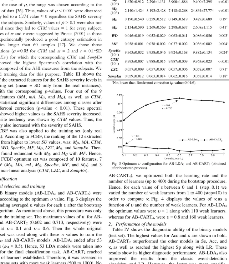
The AB binary models (AB-LDA2 and AB-CART2) were
selected according to the optimum value. Fig. 3 displays the corresponding averaged values for each after the bootstrap 0.632 algorithm. As mentioned above, this procedure was only applied to the training set. The maximum values of for AB-LDA2 and AB-CART2 (0.602 and 0.713, respectively) were
reached at = 0.1 and = 0.6. Then the whole original training set was used along with these values to train the AB-LDA2 and AB-CART2 models. AB-LDA2 ended after 53
iterations (54 ≥ 0.5). Hence, 53 LDA models were taken into
account for the final classification task. AB-CART2 reached
the limit of learners established. Therefore, it was assessed in the bootstraps sets with more weak learners (500 to 1000). No improvement in was reached. Consequently, the weighted votes of 400 CART models were used for the classification.
For the case of the AB multiclass models (AB-LDA4 and
AB-CART4), we optimized both the learning rate and the
number of learners (up to 400) during the bootstrap procedure. Hence, for each value of between 0 and 1 (step=0.1) we varied the number of weak learners from 1 to 400 (step=10) in order to compute Fig. 4 displays the values of as a function of and the number of weak learners. For AB-LDA4
the optimum values were = 1 along with 110 weak learners, whereas for AB-CART4, were = 0.8 and 160 weak learners.
2) Performance of the models
Table IV shows the diagnostic ability of the binary models (test set). The highest values for Acc and are shown in bold. AB-CART2 outperformed the other models in Se, Acc, and
as well as reached the highest Sp along with LR. These results show its higher diagnostic performance. AB-LDA2 also
improved the results from the classic event-detection algorithm and LR. However, the latter was more specific. Additionally, AB-LDA2 and AB-CART2 widely improved the
performance of single models based on LDA and CART (LDA2 and CART2).
Fig. 3 Optimum configuration for AB-LDA2 and AB-CART2 (obtained
The lowest performance was reached by the algorithm based on the event-detection approach.
In the multiclass task, Table V displays the confusion matrices of each model, i.e., the model class estimation for each subject vs. their actual SAHS severity group. Notice that, since it is a binary classifier, LR was evaluated following the one vs. all strategy [41]. The overall accuracy (main diagonal) of the models and the event-detection algorithm was low in test set: event-detection 39.7%, LR 57.4%, AB-LDA4 60.3%
(47.6 % in the case of a single LDA4 model), and AB-CART4
57.4% (54.8 % in the case of a single CART4 model).
Classification of mild and moderate subjects was particularly poor for all the models. In contrast to the overall accuracy, the diagnostic performance increases when assessing the predictions of the models in each of the AHI severity cutoffs (5 e/h, 15 e/h, and 30 e/h). Table VI displays such performance for the multiclass models and the event-detection algorithm. Consistent with the overall accuracy, values are low. However, high diagnostic accuracies are reached by AB-LDA4 and AB-CART4. They outperformed LR and the
event-detection algorithm in terms of Acc and when assessing the three AHI cutoffs. Finally, AB-LDA4 widely improved the
overall performance of single LDA4, as well as the Acc for
each AHI cutoff. AB-CART4 also improved the overall
performance of CART4, as well as the Acc for 5 e/h and 30
e/h. However, CART4 outperformed the Acc of AB-CART4
when considering 15 e/h as the AHI cutoff.
V. DISCUSSION AND CONCLUSIONS
In this paper, new methodologies to help in SAHS diagnosis have been proposed. Binary and multiclass AB models, composed of LDA and CART classifiers, have been evaluated to distinguish SAHS and its severity. Their performances were compared with a conventional approach (event-detection algorithm) and the classic LR classifier, both of them applied to our own database. AB outperformed these, showing high diagnostic ability.
Spectral and non-linear data, extracted from single-channel AF from NPP, were the only source of SAHS-related information used to feed the models. The spectral analysis showed significantly higher spectral power (Mf1) and power
spectral density (MA and mA) in the 0.025-0.050 Hz. frequency band as SAHS severity increased. Since we
TABLE IV
DIAGNOSTIC ABILITY OF THE BINARY MODELS IN THE TEST SET
Models Se (%) Sp (%) Acc (%)
Event-detec. 75.8 54.3 69.0 0.286
LR 83.5 80.0 82.5 0.593
LDA2 72.5 74.3 73.0 0.410
CART2 85.7 68.6 81.0 0.593
AB-LDA2 86.8 77.1 84.1 0.618
AB-CART2 89.0 80.0 86.5 0.672
Fig. 4 Optimum and number of weak learners for a) AB-LDA4 and b) AB-CART4 (obtained after the bootstrap process).
TABLE V. CONFUSION MATRICES FOR EACH MODEL IN THE TEST SET. RESULTS FROM LDA AND CART SINGLE MODELS IN PARENTHESES.
Estimated →
Event-detection LR (one vs. all) AB-LDA4 (LDA4) AB-CART4 (CART4)
no mild mod. severe no mild mod. sever e
no mild mod. severe no mild mod. severe
A
ct
ual
no-SAHS 2 4 3 1 8 0 2 0 8 (8) 0 (0) 2 (2) 0 (0) 8 (7) 1 (2) 1 (1) 0 (0)
mild 12 16 5 5 14 8 10 6 11 (13) 16 (7) 8 (13) 3 (5) 14 (16) 8 (11) 12 (9) 4 (2)
moderate 1 5 5 5 3 3 4 6 3 (5) 4 (2) 6 (6) 3 (3) 3 (4) 2 (3) 6 (6) 5 (3)
severe 3 17 15 27 2 1 7 52 1 (4) 3 (5) 12 (14) 46 (39) 0 (3) 3 (0) 9 (14) 50 (45)
TABLE VI. DIAGNOSTIC ABILITY OF THE MULTICLASS MODELS IN THE TEST SET. RESULTS FROM LDA AND CART SINGLE MODELS IN PARENTHESES.
Event-detection LR (one vs. all) AB-LDA4 (LDA4) AB-CART4 (CART4)
5 15 30
Se (%) 86.2 66.7 43.5 83.6 88.5 83.9 87.1 (81.0) 85.9 (79.5) 74.2 (62.9) 85.3 (82.8) 89.7 (87.2) 80.6 (72.6) Sp (%) 20.0 70.8 82.8 80.0 62.5 81.3 80.0 (80.0) 72.9 (58.3) 90.6 (87.5) 80.0 (70.0) 64.6 (75.0) 85.9 (92.2) Acc (%) 81.0 68.3 63.5 83.3 78.6 82.5 86.5(81.0) 81.0 (71.4) 82.5 (75.4) 84.9 (81.7) 80.2 (82.5) 83.3 (82.5)
normalized the PSD values, these measures are related to a higher occurrence of the apneic events, and not with their amplitude. This supports these features as SAHS severity dependents. Dispersion (Mf2) in the PSDn values at BW was
also significantly higher as SAHS worsened, suggesting a more heterogeneous occurrence of apneic events throughout the frequencies within BW. Finally, the non-linear analysis showed significantly higher variability (lower CTM values) when SAHS severity increased. This is consistent with our initial assumption that the more severe SAHS the more changes in the respiratory pattern and, consequently, the higher variability in AF. These five features were selected by FCBF. Although Mf2, SpecEn, MF, LZC, and SampEn did not
show discriminative power to distinguish SAHS severity, they were also automatically chosen, suggesting their usefulness by providing complementary information. Moreover, spectral and non-linear features were included in the 10-feature FCBF optimum set, which indicates that one analysis complement the other, as suggested in previous studies involving AF from thermistor [17], [18].
AB-CART2 achieved the highest Acc and values for the
binary (AHI cutoff = 10 e/h) classification task (86.5% Acc, 0.672 ). In the multiclass classification, AB-LDA4 obtained
86.5%, 81.0%, 82.5% Acc for 5 e/h, 15 e/h, and 30 e/h, respectively, as well as = 0.432. It is worth noting that both AB-LDA4 and AB-CART4 reached high statistics when
evaluating 5 e/h and 30 e/h. They outperformed the LR models, the single-model LDA and CART classifiers, as well as the event-detection algorithm. These cutoffs are particularly important. AHI = 5 e/h draws the line for the lower degree of SAHS. Furthermore, AHI = 30 e/h, which establish the boundary for the highest SAHS severity, has been associated with mortality [49], as well as suffices to recommend a treatment even in the absence of other symptoms [49]. In this regard, and according to Table V, 46 out of the 52 subjects (88.5 %) that the AB-LDA4 ensemble predicted as
severe-SAHS were rightly classified, whereas the remaining 6 (11.5%) were mild- or moderate-SAHS, at least. Similarly, 50 out of the 59 subjects (84.7%) that the AB-CART4 ensemble
predicted as severe were indeed severe, with 0 subjects from the no-SAHS group falling within this class.
Table VII summarizes performances from previous works focused on the use of single-channel AF from NPP to help in SAHS diagnosis [10], [13], [50]-[52]. All studies, except the present one, adopted an event detection approach. When assessing AHI = 10 e/h, only Wong et al achieved higher diagnostic performance than AB-CART2 [10], [51]. However,
a small sample size was used to evaluate their proposals. Nakano et al detected apneic events in AF with the help of spectral analysis [50]. They reported higher Se (97.0%) but lower Sp (76.0%). Unfortunately, some data about the population under study, required to complete the comparison, were not reported by the authors. None of the studies, outperformed our AB-LDA4 model (86.5% Acc) in the
assessment of AHI = 5 e/h. However, Nakano et al reported significantly higher Se (97.0%) [50]. Additionally, BaHammam et al and Nigro et al exhibited higher diagnostic
ability when assessing AHI = 30 e/h [13], [52]. Nonetheless, their databases were composed of 95 and 90 subjects, respectively, in contrast to the 317 subjects involved in our study. Finally, all the studies performed similarly to our AB-LDA4 model (81.0% Acc) when evaluating AHI = 15 e/h.
Despite we have shown the utility of our proposal, some limitations need to be addressed. Although our sample is large (317 subjects), analyzing more recordings would enhance the statistical power of our results. Particularly, a more balanced proportion of the classes would be desirable for the sake of the model training. Nonetheless, our sample reflects a realistic proportion among the people who undergo the PSG test. Additionally, we applied the SMOTE technique to our data in order to compensate the imbalance. The single use of NPP to acquire AF may be another limitation. The AASM recommends using both NPP and thermistor for a proper quantification of the number of apneas and hypopneas [9]. However, our proposal does not rely on a classic event-detection approach. In this regard, previous studies of our research group showed high diagnostic ability when evaluating data from single-channel AF acquired through a thermistor [17], [18]. Our current proposal has shown that using AF data from NPP is also possible in order to reach a high diagnostic performance. Another limitation arises regarding the redundant information removed by the FCBF algorithm. The features discarded share more information with the selected ones than with the AHI. However, the features selected might still share information with the others to some extent. The training time of the AdaBoost models is another limitation if we compare it with simpler methodologies such as logistic regression. However, once the models are trained, the runtime after they are applied to new data is trivial. Finally, since we propose an automatic procedure with potential to reach diagnosis in few minutes after data collection, it would be of great interest if future works could
TABLE VII
COMPARISON WITH THE STATE OF THE ART OF SINGLE-CHANNEL AF FROM NPP
Studies Subjects
(n)
AHI cutoff Se (%) Sp (%) Acc (%) aDe Almeida et al
[10] 30 10 85.7 87.5 nd
aNakano et al
[50] 217
5 97.0 77.0 nd
10 97.0 76.0 nd
15 97.0 73.0 nd
aWong et al
[51] 33
10 92.0 86.0 90.9*
30 91.0 75.0 81.5*
aBaHammam et
al [52] 95
5 79.0 68.0 76.8*
10 70.0 89.0 77.9*
15 65.0 94.0 81.8*
30 63.0 98.0 83.2*
aNigro et al
[13] 90
5 89.3 60.0 84.4*
10 80.4 82.3 nd
15 76.7 83.0 80.0*
30 88.5 95.3 93.3*
bAB-CART
2 317 10 89.0 80.0 86.5
bAB-LDA
4 317
5 87.1 80.0 86.5
15 85.9 72.9 81.0
30 74.2 90.6 82.5
address the assessment of our methodology embedded in a diagnostic test at patient’s home. It would be also interesting the implementation and assessment of a multiclass logistic-regression based AdaBoost algorithm.
To the best of our knowledge, this is the first time that the AB algorithm is used along with spectral and nonlinear features from single-channel AF to help in SAHS diagnosis. Our AB proposals for binary and multiclass classification outperformed the classic LR as well as a conventional event-detection algorithm, both of them applied to our own database. The new AB-CART2 and AB-LDA4 models achieved high
diagnostic ability compared with the state of the art. Additionally, we showed that it is possible to achieve high diagnostic ability by the use of spectral and nonlinear data from NPP AF. These results highlight the usefulness of our proposal when detecting SAHS and its severity.
REFERENCES
[1] T. Young et al, “Epidemiology of Obstructive Sleep Apnea: A Population Health Perspective,” Am. J. Respir. Crit. Care. Med., vol. 165, pp. 1217-1239, 2002.
[2] F. Lopez-Jiménez et al, “Obstructive Sleep Apnea,” Chest, vol. 133, pp 793-804, 2008.
[3] S. P. Patil, et al, “Adult Obstructive Apnea,” Chest, vol. 132, pp. 325-337, 2007.
[4] A. Sassani, et al, “Reducing Motor-Vehicle Colissions, Costs, and Fatalities by Treating Obstructive Sleep Apnea Syndrome,” Sleep, vol. 27, pp. 453-458, 2003.
[5] E. Lindberg et al, “Role of Snoring and Daytime Sleepiness in Occupational Accidents,” Am. J. Respir. Crit. Care Med., vol. 164, pp. 2031-2035, 2001.
[6] F. Campos-Rodriguez et al, “Association between obstructive sleep apnea and cancer incidence in a large multicenter spanish cohort,” Am. J. Respir. Crit. Care Med., vol. 187, pp. 99-105, 2013.
[7] J. A. Bennet and W. J. M. Kinnear WJM, “Sleep on the cheap: the role of overnight oximetry in the diagnosis of sleep apnoea hypopnoea syndrome,” Thorax vol. 54, pp. 958-959, 1999.
[8] W. W. Flemons et al, “Home Diagnosis of Sleep Apnea: A Systematic Review of the Literature,” Chest, vol. 124, pp. 1543-1579, 2003. [9] R. B. Berry et al, “Rules for scoring respiratory events in sleep: update
of the 2007 AASM manual for the scoring of sleep and associated events,” J. Clin. Sleep Med., vol. 8(5), pp. 597-619, 2012.
[10] F. R. de Almeida et al, “Nasal pressure recordings to detect obstructive sleep apnea,” Sleep Breath, vol. 10, pp. 62-69, 2006.
[11] U. J. Magalang et al, “Prediction of the apnea-hypopnea index from overnight pulse oximetry,” Chest, vol. 124, pp. 1694-1701, 2003. [12] T. Penzel et al, “Systematic Comparison of Different Algorithms for
Apnoea Detection Based on Electrocardiogram Recordings,” Med. Biol. Eng. Comput., vol. 40, pp. 402-407, 2002.
[13] C. A. Nigro et al, “Comparison of the automatic analysis versus the manual scoring from ApneaLink™ device for the diagnosis of obstructive sleep apnoea syndrome,” Sleep Breath vol. 15, pp. 679-686, 2011.
[14] C. Gómez et al, “Complexity analysis of the magnetoencephalogram background activity in Alzheimer's disease patients,” Med. Eng. Phys., vol. 28, pp. 851-59, 2006.
[15] D. Álvarez et al, “Multivariate analysis of blood oxygen saturation recordings in obstructive sleep apnea diagnosis,” IEEE Trans. Biomed. Eng., vol. 57, no. 12, pp. 2816–2824, 2010.
[16] J. V. Marcos et al, “Automated detection of obstructive sleep apnea syndrome from oxygen saturation recordings using linear discriminant analysis,” Med. Eng. Phys., vol. 59, pp. 141-49, 2010.
[17] G. C. Gutiérrez-Tobal et al., “Pattern recognition in airflow recordings to assist in the sleep apnoea–hypopnoea syndrome diagnosis,” Med. Biol. Eng. Comput., vol. 51, pp. 1367-80, 2013.
[18] G. C. Gutiérrez-Tobal et al, “Linear and nonlinear analysis of airflow recordings to help in sleep apnoea-hypopnoea syndrome diagnosis,” Physiol. Meas., vol. 33, pp. 1261-75, 2012.
[19] R. Hornero et al, “Spectral and nonlinear analyses of MEG background activity in patients with Alzheimer's disease,” IEEE Trans. Biomed. Eng., vol. 55, pp. 1658-1665, 2008.
[20] L. Yu and H. Liu, “Efficient feature selection via analysis of relevance and redundancy,” J. Mach. Learn. Res., vol. 5, pp. 1205-1224, 2004. [21] A. Aarabi et al, “Automated neonatal seizure detection: A multistage
classification system through feature selection based on relevancy and redundancy analysis,” Clin. Neurophysiol., vol. 117, pp. 328-340, 2006. [22] I. H. Witten, E. Frank and M. A. Hall, Data Mining: Practical Machine
Learning Tools and Techniques. Burlington, MA: Morgan Kaufmann/Elsevier, 2011.
[23] C. Morgenstern et al, “Assessment of changes in upper airway obstruction by automatic identification of inspiratory flow limitation during sleep,” IEEE Trans. Biomed. Eng., vol. 56, pp. 2006-2015, 2009. [24] B. Xie and H. Minn, “Real-time sleep apnea detection by classifier
combination. Information Technology in Biomedicine,” IEEE Trans. Biomed. Eng., vol. 16, pp. 469-477, 2012.
[25] W. W. Flemons et al, “Access to diagnosis and treatment of patients with suspected sleep apnea,” Am. J. Respir. Crit. Care. Med., vol. 169, pp. 668-72, 2004.
[26] N. V. Chawla et al, “SMOTE: synthetic minority over-sampling technique,” J. Artif. Intell. Res., vol. 16(1), pp. 321-357, 2002.
[27] J. Han et al, “Detection of apnoeic events from single channel nasal airflow using 2nd derivative method,” Comput. Meth. Prog. Bio., vol. 98, pp. 199-207, 2008.
[28] A. Qureshi et al, “Obstructive sleep apnea,” J. Allergy Clin. Immunol., vol. 112, pp. 643-651, 2003.
[29] A. S. Karunajeewa et al, “Multi-feature snore sound analysis in obstructive sleep apnea–hypopnea syndrome,” Physiol. Meas., vol. 32(1), pp. 83, 2011.
[30] P. D. Welch, “The Use of Fast Fourier Transform for the Estimation of Power Spectra: A Method Based on time Averaging Over Short, Modified Periodograms,” IEEE Trans. on Audio and Electroacoustics, vol. AU-15, pp. 70-73, 1967.
[31] L. Sörnmo and P. Laguna, Bioelectrical signal processing in cardiac and neurological applications. London, U.K./New York: Elsevier/Academic; 2005.
[32] D. J. Eckert and A. Malhotra, “Pathophysiology of adult obstructive sleep apnea,” Proc. Am. Thorac. Soc., vol. 5, pp. 144-153, 2008. [33] J. Poza et al, “Extraction of spectral based measures from MEG
background oscillations in Alzheimer's disease,” Med. Eng. Phys., vol. 29, pp. 1073-1083, 2007.
[34] W. K. Wootters, “Statistical distance and Hilbert space,” Physical Review D, vol. 23(2), pp. 357-362, 1981.
[35] M. T. Martin et al, “Statistical complexity and disequilibrium,” Physics Letters A, vol. 311(2), pp. 126-132, 2003.
[36] M. E. Cohen et al, “Applying continuous chaotic modeling to cardiac signal analysis,” IEEEEng. Med. Biol. Mag., vol. 15, pp. 97-102, 1996. [37] D. Abásolo et al, “Analysis of EEG background activity in Alzheimer's
disease patients with Lempel–Ziv complexity and central tendency measure,” Med. Eng. Phys., vol. 28(4), pp. 315-322, 2006.
[38] J. Ziv and A. Lempel, “Compression of individual sequences via variable-rate coding,” IEEE Trans. Inform. Theory, vol. 24, pp. 530-536, 1978.
[39] D. Abásolo et al, “Entropy analysis of the EEG background activity in Alzheimer's disease patients.” Phys.Mmeas., vol. 27, pp. 241-253, 2006. [40] J. S. Richman and J. R. Moorman, “Physiological time-series analysis
using approximate entropy and sample entropy,” Am. J. of Physiol-Heart C., vol. 278, pp. H2039-H2049.
[41] C. M. Bishop, Pattern Recognition and Machine Learning. New York, NY: Springer, 2006.
[42] Y. Freund, and R. E. Schapire, “A decision-theoretic generalization of on-line learning and an application to boosting”, J. Comput. System Sci., vol. 55(1), pp. 119-139, 1997.
[43] J. H. Friedman, “Greedy function approximation: a gradient boosting machine,” Annals of Statistics, 1189-1232, 2001.
[44] D. W. Hosmer and S. Lemeshow, Applied Logistic Regression. New York, NY: John Wiley and Sons, 2000.
[45] J. B. Korten and G. G. Haddad, “Respiratory waveform pattern recognition using digital techniques,” Comput. Biol. Med., vol. 19, pp. 207-217, 1989.
[46] B. Efron and R. J. Tibshirani, An introduction to the bootstrap. CRC press, 1994.
[48] N. M. Punjabi et al, “Sleep-disordered breathing and mortality: a prospective cohort study,” PLoS medicine, vol. 6(8), pp. e1000132, 2009.
[49] P. Lloberes et al, “Diagnosis and treatment of sleep apnea-hypopnea syndrome,” Arch. Bronconeumol. ((English Edition)), vol. 47(3), pp. 143-156, 2011.
[50] H. Nakano et al, “Automatic Detection of Sleep-disordered breathing from a single-channel airflow record,” Eur. Respir. J., vol. 29, pp. 728-736, 2007.
[51] K. K. Wong et al, “Diagnostic test evaluation of a nasal flow monitor for obstructive sleep apnea detection in sleep apnea research,” Behavior research methods, vol. 40(1), pp. 360-366, 2008.