Commodity prices shocks and the balance sheet effect in Latin America

(1)

Commodity Prices Shocks and the Balance Sheet Effect in

Latin America

Laura Wberth Escobar∗ Alejandro Torres Garc´ıa, Ph.D.†

Abstract

Emerging market economies (EMEs), particularly the commodity exporter ones, are ex-posed to world’s dynamics through different channels. In this paper, we consider the role of (exogenous) commodity prices shocks in explaining business cycles in EMEs, by propos-ing a financial transmission mechanism: the balance sheet effect. Our hypothesis is that firm’s external debt dynamics are related to commodity prices. To test it, we estimate a se-ries of VAR models using quarterly data on corporate external debt, nominal exchange rate, EMBI+spreads, the local currency value of external debt to nominal GDP ratio and real GDP, covering the period 2000−2017. We do this for Latin America and then, we focus on five particular economies: Brazil, Chile, Colombia, Mexico and Peru. We find that balance sheets do matter and they exacerbate the output’s contraction when the commodity price shock is negative. We also find that, turning the financial channel off, the real GDP cumu-lative response in Latin America is half smaller than in the unrestricted model. We find no evidence on the existence of the balance sheet effect for Chile.

I

Introduction

Latin American economies, to different extent, are characterized for being strongly dependent on their natural resources endowment. Their export basket is mainly composed by

commodi-ties such as oil, hydrocarbon, minerals and some agricultural raw materials. Although com-modities’ share on total exports has reduced from the 1970s decade, it remains relatively large compared to other regions (Sinnott et al., 2010).

This commodity dependence implies that Latin American countries are subject to world’s

commodities prices dynamics, leaving them exposed to their volatility. Being determined by supply and demand interaction, commodities prices tend to be highly variable, which could affect not only the primary sector but its effects spread to the entire economy. As a matter of

fact, Mendoza (1995), and more recently, Vegh et al. (2017) state that commodity prices can be

(2)

a potential cause for business cycles in developing economies.

This dependency was specially clear in the middle of the last commodity prices boom, that started in the early 2000sand finished approximately in 20141, and allowed some Latin

Amer-ican countries to benefite from this boom. In fact, average economic growth in Brazil, Chile, Colombia, Mexico and Peru, in period 2002−2013 was 4.60%. With the end of the boom came

a reduction in average growth rate in this same group: 1.72% between 2014 and 2016.

What can be expected when commodity prices fall? Knowing that commodity-exporting economies tend to attract foreign investment in their primary sector, an effect of volatility in

commodity prices is that it may induce variability in nominal exchange rate related to capital flows (Reinhart et al., 2016). Particularly, when commodity prices decrease so does profitability in that sector, which may induce a nominal exchange rate depreciation.

Conventional textbook wisdom highlights the advantages of devaluations, arguing that

they stimulate economic growth through an increase in exports and, since imported goods are relatively more expensive, consumers tend substitute them for locally produced goods2, which also enhances domestic demand. Nevertheless, this is not the whole story and there are other

effects of exchange rate increases.

An under-studied impact of depreciations is the one related to balance sheets of companies and governments that possess debt denominated in foreign currency (C´espedes et al., 2004). In

this context, depreciation in exchange rates raises the local currency value of companies’ total owing balance overnight, forcing them to make higher efforts to meet debt-service payments. Thisvalue effectimplies that investment decisions inside companies might be disturbed,

hav-ing undesirable effects for the firm, in particular, and the aggregate economic activity overall. As authors explain, the currency mismatch between revenues and liabilities can cause

depreci-ation to be contractionary instead of expansionary, as the conventional wisdom states.

In this sense, balance sheet effects constitute a sort of financial accelerator that can deepen business cycles and increase their volatility. Anytime commodity prices rise, the increased for-eign indebtedness may lead to an even higher expansion in output. In contrast, when these

prices fall, balance sheet effects might accentuate the bust through the aforementioned invest-ment reductions.

1_{Regarding to this episode, Gruss (2014) states that “oil prices in current U.S. dollars almost quadrupled between}

2003 and 2013 and metal prices tripled, while food prices doubled and prices of agricultural products rose by about

50 percent” (pp. 6)

2_{An important point here to take into account is that all goods are not easily substituted, like capital goods, for}

(3)

At the same time, there is another consequence of variability in commodity prices.

Con-sidering that interest rate risk premium in commodity-exporting economies may be strongly related to commodity prices, it follows their volatility also affects the borrowing cost (interest

rate spread) faced by entrepreneurs in such countries (Malone, 2009). Since a decrease in com-modity prices lowers profitability in these sectors and the entire economy is perceived as less attractive, this may end up increasing the interest rate spread, due to a higher default

probabil-ity: the increased cost of borrowing ultimately hinders new debt acquisition by entrepreneurs. This can be thought of as aquantity effect.

Now, bearing all this in mind, it makes sense to explore the effects that commodity prices

shocks have on entrepreneurs’ balance sheets. It is important to highlight that enterprises do not need to be on the primary sector to be affected by the aforementioned shocks through the nominal exchange rate fluctuations. This issue can be approached following C´espedes et al.

(2004), whom develop a theoretical model where risk premium is a function of entrepreneurs’ value of investment relative to net worth. Gertler et al. (2007) also constitute a relevant

refer-ence to answer our question, since they use a model similar to the one in C´espedes et al. (2004) to explain the Korean crisis.

Regarding to the effects of exchange rate fluctuations in companies’ balance sheets, most economic researches have focused at the micro level3_{. Evidence on the existence of balance}

sheet effects related to exchange rate depreciation is mixed, although this literature has been able to establish a negative correlation between exchange rates and firm’s investment. To the

best of our knowledge, little has been done to assess this matter at the macroeconomic level nor to connect it to commodity prices fluctuations.

All of the above displays an interesting research question to be answered in this paper. So our main goal is to provide a different, sometimes ignored, cause for business cycles in

de-veloping countries. We aim to untangle the linkage between the last commodity prices boom (period 2002−2014) and the existence of balance sheet effects in Latin America and five

par-ticular economies: Brazil, Chile, Colombia, Mexico and Peru.

To achieve our goal, we estimate a serie of VAR models, with a conceptual framework

pro-vided by C´espedes et al. (2004), using quarterly data of commodity prices, nominal exchange rate, EMBI spreads, external debt and real GDP data. One finding is that balance sheets are

important business cycles drivers in the region. Particularly, half of the output contraction is due to firm’s debt dynamics. Also, the behavior of Brazil, Colombia, Mexico and Peru is well represented by the region.

3_{Bonomo et al. (2003), Benavente et al. (2003), Echeverry et al. (2003), Lobato et al. (2003) and Carranza et al.}

(4)

Another finding is that Chilean economy is significantly different from its counterparts and

the region. For this economy, real copper price seems not to be a key business cycle driver and balance sheet effect is actually negligible. We believe this result is explained by Chilean

insti-tutional structure and, especially, the existence of the economic and social stabilization fund (ESSF) and fiscal rules.

This paper is organized in five sections, including this introduction. In section 2, we discuss how economic literature approaches commodity prices shocks and business cycles in emerging

economies and the balance sheet effect. In section 3, we describe our data and explore some stylized facts for Latin America in general and the five studied countries in particular. Section

4 explains our methodology and presents estimation results. Finally, section 5 concludes.

II

Commodity Prices, Interest Rates and Balance Sheet Effects

There is a vast economic literature4 _{exposing the connection between commodity prices (or}

terms of trade) and real GDP cycles in EMEs, considering mainly real and commercial chan-nels. Fern´andez et al. (2017a) model explicitly the transmission mechanisms of commodity

prices shocks to the real sector, through their effects on domestic goods demand, using a dy-namic stochastic equilibrium model. Two stylized facts found by authors is that commodity

prices have a strong comovement with other macroeconomic variables. As a matter of fact, they find that commodity prices are procyclical and leading to output, investment and con-sumption. Moreover, authors also find that commodity prices are countercyclical to real

ex-change rates and external risk premium.

The model considers an endowment commodity sector that faces fluctuations on its interna-tional price, which it is taken as given by households. The model has four agents: households, firms (domestic good producers), investment good producers and the rest of the world.

For-eign and home goods are used as inputs in investment goods production and are also imperfect substitutes in the consumption. Households offer labor services in the labor market and they

own commodity endowment, receiving commodity revenues. Firms produce domestic goods using labor and capital inputs.

In this framework, households can issue bonds in international financial markets, where they pay a spread over international interest rate. These two variables are considered

exoge-nous and stochastic, being other business cycle forces. Additionally, authors propose that com-modity prices are composed by a latent common factor and idiosyncratic shocks. In the model,

the only source of fluctuations in commodity prices is related to shocks to the common factor. Equation 1 presents the log-linearized version of market clearing condition, which allows to

4_{See, for example, Fern´andez et al. (2017b), Shousha (2016), Kose (2002), Tretvoll et al. (2017) and Charnavoki}

(5)

decompose the real GDP response to a positive shock in the commodity price’s common factor,

as the sum of three effects:

yt =

Ch

Y

ch_t

| {z }

E f f ect1 +

Xh

Y

xh_t

| {z }

E f f ect2 +

Ch∗

Y

ch_t∗

| {z }

E f f ect3

(1)

where letters without subscript represent steady state levels. Yis output,Chis home good

consumption, Xh is domestic good used in investment good production and Ch∗ is external demand for home goods. Lower-case letters represent log deviations from steady state levels (xt= ln(Xt)−ln(X)). Effect 1 embodies adomestic demand channel: the positive commodity

income shock leads households to increase their demand. Domestic relative prices increase in response to this to stimulate production.

Effect 2 accounts for changes in new investment goods. On the one hand, to meet the

in-creased domestic demand, firms increment their capital demand and hence, its rental rate. On the other hand, demand for new investment goods also increases, and so does its price. Alto-gether, this constitutes a greater expansion in demand for domestic goods.

Lastly, effect 3 is related to the response of external demand for home goods. Given that the

commodity income boom induces an increase in domestic prices, the economy is less compet-itive in international markets. This way, home goods become relative more expensive, which

detriments its demand from foreigners.

The net effect of the commodity shock in aggregate output will depend on the strength of

the aforementioned effects. In turn, every effect depends on economy’s structural parameters describing firms, households and investment goods producers behavior. Assuming that effect

3 is not large enough to counterbalance effects 1 and 2, the net effect is positive and, in the new equilibrium, real exchange rate appreciates5. Lastly, in the empirical strategy, authors find that

the model replicates correctly patterns depicted by EMEs data, particularly those from Brazil, Chile, Colombia and Peru.

As a final remark regarding to Fern´andez et al. (2017a) model, it is worth noting that interest rates spreads are not explicitly modeled as a function of commodity prices. Furthermore, this

model does not consider the external debt dynamics nor the currency mismatch problems that could take place between households’ incomes and liabilities. Nevertheless, this paper makes clear the connection between commodity prices and real output in EMEs.

5_{A reasonable conclusion is that, given the economic structure modeled, a fall in commodity prices would cause}

a depreciation in exchange rates. Besides, the net effect in output would depend on the relative strength of

(6)

The financial channel or balance sheet effect of debt denominated in foreign currency has

been approached in the economic literature as a phenomenon related of external interest rates shocks. In this sense, C´espedes et al. (2004) develop a theoretical model with financial

fric-tions6where debt is dollarized and country risk premium is endogenous. Authors show how devaluations in exchange rate can be detrimental for economic performance, which contradicts conventional textbook wisdom.

In this context, authors solve the financial contract problem between domestic entrepreneurs

and foreign lenders. In doing so, they make an extension to Bernanke et al. (1999) in an open economy context to find a critical equation that guarantees interest rates parity:

Et(Rt+1Kt+1/St+1) QtKt+1/St

= (1+ρt+1)(1+ηt+1) (2) Equation 2 equalize the expected return on the entrepreneur’s investment project and the international safe interest rate (1+ρt+1). Entrepreneurs must pay a spread over the interna-tional interest rate, ηt+1 or risk premium, that reflects the informational asymmetries in the financial contract enforcement. Now, in equilibrium, entrepreneur’s net worth, denominated

in local currency, is7:

Nt =δ[(1−Φt)αYt−(1+ρt)EtDt] (3)

whereEt =St/Ptis the real exchange rate,δis the unconsumed proportion of entrepreneur’s

net worth and(1−Φ_t)reflects monitoring costs paid in the contract enforcement. What is

in-teresting in equation 3 is that, given real income, Yt, and contemporaneous risk premium, a

real devaluation impacts negatively entrepreneur’s net worth because it increases the burden of interest payments associated to inherited debt.

Akey featureof C´espedes et al. (2004) model is that risk premium is an increasing function

of the investment cost-net worth ratio, as shown by Bernanke et al. (1999):

1+ηt+1= F

QtKt+1 PtNt

, F(1) =1, F0(·)>0 (4)

The functional form of risk premium, displayed in equation 4, incorporates the balance

sheet effects in the model. This effect is related to investment decisions in a firm that possess debt denominated in foreign currency: whenever exchange rate depreciates, the local currency value increases and so does interest payments. If the firm obtains revenues in local currency,

automatically it has to make a higher effort to repay its debt, forcing it to reduce investment and hence, production.

6_{In their model, financial frictions are due to informational or enforcement problems.}

(7)

Particularly, authors are interested in studying the effects of an unanticipated and

tempo-rary increase in the safe interest rate,ρt+1, under both flexible and fixed exchange rate regimes. This shock causes an increase in exchange rate. Authors find that balance sheet effects are

relevant and can actually amplify the effects of foreign disturbances. As a matter of fact, this magnification is particularly sharp when the economy is financially vulnerable and the con-ventional effect of depreciation in exchange rate is overshadowed by the financial effect.

A model in the same strand as C´espedes et al. (2004) is the one of Gertler et al. (2007), who

propose a financial accelerator model, where exchange rate regime is linked to financial dis-tress, to explain the South Korean crisis of 1997−1998. Authors explain that Korean crisis was

triggered by a reduction in country’s sovereign risk status made by Standard & Poor’s. This caused a capital flight and a sharp increase in country risk premium. In turn, to maintain fixed exchange rates, central bank responded raising interest rates. This response combined with a

higher country risk, ultimately were translated in a deterioration of economic activity.

The financial accelerator mechanism proposed by authors connects borrower balance sheets to the external risk premium in the financial contract. Agents interacting in the model are: households, firms (entrepreneurs, capital producers and retailers) and a government. As in

Fern´andez et al. (2017a), there are both domestic and foreign goods that are imperfect sub-stitutes. In this model, the country borrowing premium for external debt is a function of net

foreign indebtedness,NFt, and a random shock,Φt:

Ψt = f(NFt)Φt, with f0(·)>0 (5)

Authors claim that this specification of borrowing premium is useful since it helps to

repli-cate the apparent cause of Korean crisis. They associate the capital flight observed to an increase in the random variableΦt.

On the production side, entrepreneurs are the key players. To carry out production, they

must finance their capital demand through their own net worth of the end of periodt, Nt+1,

and nominal bonds,Bt+1. In this context, entrepreneurs and lenders solve a financial contract with costly bankruptcy yielding a financial premium, given by:

χt(·) =χ



  

Bt+1 Pt

Nt+1 

  

, χ

0

(·)>0, χ(0) =0, χ(∞) =∞ (6)

It is clear, from equation 6, that the financial premium faced by entrepreneurs is an increas-ing function of their leverage ratio: the higher this ratio is, the higher interest rate entrepreneurs

(8)

Now, how does the shock on country risk premium, i.e., an increase in equation 5 trigger

the financial accelerator mechanism and affect output? The massive capital outflow caused an increase in nominal exchange rates by central bank, in order to protect the fixed exchange rate.

Given nominal rigidities in the retail sector, real interest rate also rose, inducing a contraction in output. This is exaggerated by the financial accelerator mechanism: the higher real inter-est rate generates a reduction in asset prices, which in turn, reduces entrepreneurs’ net worth

and hence, increases their leverage ratio. As stated by equation 6, a higher leverage raises en-trepreneurs’ financial premium, which ultimately leads to a reduce in investment and a sharper

output contraction.

Although initially authors consider the case when these bonds are in domestic currency, they extend their model in order to account for what happens when debt is denominated in foreign currency. One interesting finding is that the contraction in investment after the shock is

almost twice bigger when the debt is denominated in foreign currency than in the unrestricted case. Furthermore, as in C´espedes et al. (2004), Gertler et al. (2007) find that flexible exchange

rates are more desirable in terms of the output contraction, in contrast to the fixed exchange rate regime. This means that the financial accelerator mechanism is actually more detrimental in currency mismatch contexts.

We have seen that, on the one hand, commodity prices shocks are connected to output

cy-cles but that mainstream economic literature tends to leave the financial channel outside. On the other hand, the balance sheet effect has been studied under frameworks considering

inter-est rates disturbances, leaving commodity prices shocks outside. Given this, we propose that a negative shock in commodity price has the same effects as a positive shock in world safe in-terest rate, as proposed by C´espedes et al. (2004) and a positive shock in the country risk, as in

Gertler et al. (2007). Our intuition is that when commodity prices fall, the domestic economy as a whole is less attractive to foreign investors or lenders.

Lastly, an assumption we will make in our analysis, that is also found implicitly in C´espedes

et al. (2004) and Gertler et al. (2007) is that entrepreneurs can not use any financial instrument in order to cover the risk of unexpected exchange rate fluctuations, which will provide the way to connect commodity prices shocks to firm’s liabilities. This assumption makes sense in EMEs,

where financial markets are incipient and the access to its instruments is limited.

III

Data and Some Stylized Facts

Data

Firstly, we consider Latin America and then, we focuse on Brazil, Chile, Colombia, Mexico and

(9)

Panama because these are dollarized economies and Venezuela because of the political

insta-bility that characterizes this economy. Uruguay and Bolivia are excluded for data availainsta-bility. Central American countries are too small to be considered and, as stated by Sinnott et al. (2010),

these are commodity net importer economies.

We gather data from different sources. Real and nominal GDP information is collected from

CEPAL database, which provides quarterly data in local currency units. Total external debt ex-pressed in U.S. Dollars is retrieved from each country’s Central Bank. Although it is possible

that we are considering debt originally denominated in currencies different from the U.S. Dol-lar, the largest proportion of external debt in the economies we consider is, in fact, originally

denominated in dollars.

Nominal exchange rate data is also from each country’s Central Bank. Besides, we

con-struct the local currency value of external debt as the product between nominal exchange rate and dollar debt for each country. EMBI spreads data, used as a risk premium proxy, is collected

from JP Morgan and converted into quarterly data by computing daily averages. We select these variables because we are interested in studying how commodity prices shocks become affect corporate external debt and real GDP cycles, through nominal exchange rate and risk

premium.

There are differences in the time period covered: the Brazilian case is examined in the 2001Q4−2017Q2 period, while Chilean covers from 2003Q1 to 2017Q3. Colombian and Pe-ruvian cases cover the period 2000Q1−2017Q2 and Mexican data is available from 2002Q1 to

2017Q2.

To obtain data for Latin America as a whole, we considered our five countries an added Ar-gentina and Paraguay. These seven countries represent an important proportion of the entire

Latin American GDP8. External debt in dollars is added straightforward for every economy since it is all expressed in the same currency. Now, given that CEPAL reports quarterly

na-tional accounts information only in local currency, it was transformed into dollars. We did this transformation multiplying real GDP in a base period (2011Q4) by nominal exchange rate in the same period. Then, to actually obtain a GDP in constant base period dollars, we calculated

it using growth rates of real GDP in local currency units.

Nominal exchange rate index (in the Latin American case) is computed as a weighted aver-age of country-specific indexes. Here, again, base period was 2011Q4. The weights are calcu-lated as the participation of each country in the group of seven. The same procedure was used

to compute the LCU external debt to GDP ratio from every economy’s ratio data. Latin

Ameri-8_{Actually, according to World Bank data, these seven economies represent 83% of Latin American and the}

(10)

can EMBI is calculated by JP Morgan, we have this information in the period 2000Q1−2017Q1.

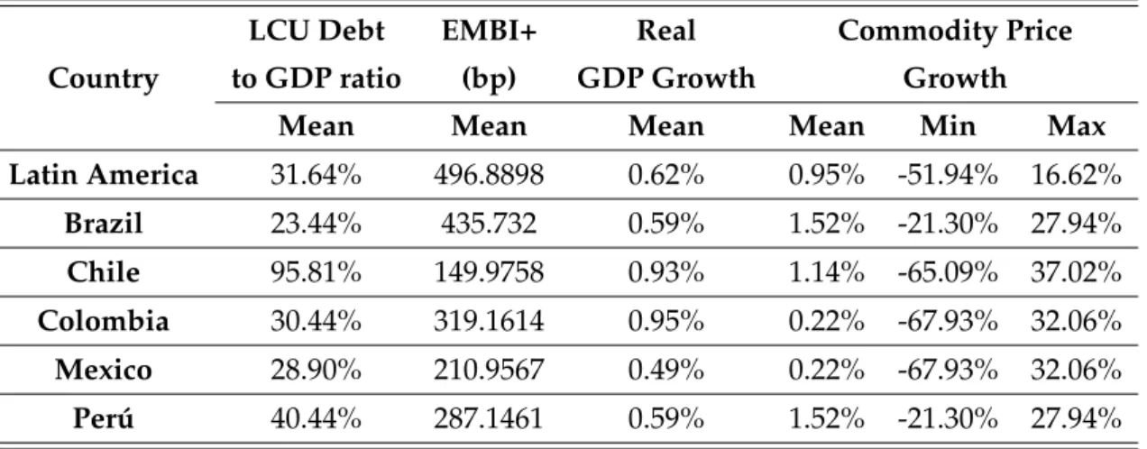
Finally, some descriptive statistics are displayed in table 1. It is noticeable that Chile has the

highest LCU debt to GDP ratio and, at the same time, the lowest EMBI+ spreads. Column 4 in table 1 exhibits quarterly GDP growth rates, where Colombia and Chile are remarkably higher than their counterparts and the region. Column 5 shows commodity prices growth,min and

maxstatistics allow us to observe their volatility.

Table 1: Descriptive Statistics - Latin America and five EMEs

Country

LCU Debt to GDP ratio

EMBI+ (bp)

Real GDP Growth

Commodity Price Growth

Mean Mean Mean Mean Min Max

Latin America 31.64% 496.8898 0.62% 0.95% -51.94% 16.62%

Brazil 23.44% 435.732 0.59% 1.52% -21.30% 27.94%

Chile 95.81% 149.9758 0.93% 1.14% -65.09% 37.02%

Colombia 30.44% 319.1614 0.95% 0.22% -67.93% 32.06%

Mexico 28.90% 210.9567 0.49% 0.22% -67.93% 32.06%

Per ´u 40.44% 287.1461 0.59% 1.52% -21.30% 27.94%

Stylized Facts

We present some empirical regularities analysis for Brazil, Chile, Colombia, Mexico and Peru compared to Latin American region. Latin American data is constructed aggregating informa-tion on output, non-financial private sector external debt, nominal exchange rate and EMBI for

our five economies plus Argentina and Paraguay.

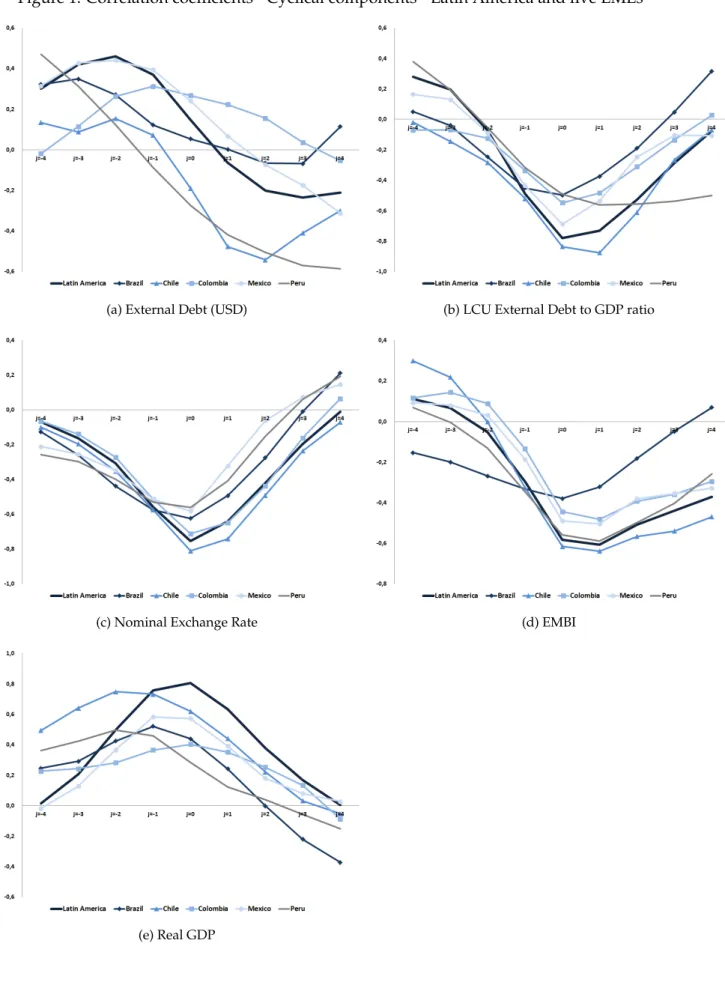
Figure 1 presents the calculated correlation coefficients9for our five EMEs and the region. These correspond to the correlation between cyclical components of every variable in periodt

and the commodity price in periodt+jwith j= −4,−3,−2,−1, 0, 1, 2, 3, 4. Regarding dollar debt (panel a), in Brazil, Colombia and Mexico the commodity-relevant price shows a procycli-cal and leading movement with respect to this variable. This means that dollar debt reacts in

the same direction and after commodity price changes. Furthermore, these economies exhibit the same behavior as Latin America. Chile and Peru behave differently from their counterparts

and the region, since the commodity price is countercyclical and lagged with respect to debt in USD, meaning that dollar debt moves before and in the opposite direction of commodity price

change.

9_{The statistical significance of these coefficients is tested, yielding that all of them are statistically different from}

(11)

Now, the commodity price is countercyclical and contemporary to LCU debt to GDP ratio

(panel b). This is the case in Brazil, Colombia, Mexico and the region. This contrasts with the Chilean and Peruvian case, where this variable is lagged. A strong finding in this paper is

the countercyclical and contemporary relation between nominal exchange rate and commodity price (panel c). This is found in the region and in the five studied economies. Considering that dollar debt is procyclical and nominal exchange rate is countercyclical, LCU debt dynamics

would initially depend on whether quantity effect is greater than the value effect explained above. Since LCU debt turned out to be countercyclical, it allows us to conclude, at least

pre-liminarily, that value effect dominates.

Regarding to EMBI spreads, our risk premium proxy, it is found that commodity price is countercyclical and has a one period lag (panel d). This is true for all economies and the region, excepting Brazil where it is contemporary. Finally, it is also clear from panel e in figure 1 that

commodity price is procyclical to GDP and contemporary for Colombia and the region, while it is leading in the other economies. This exploratory and preliminary analysis supports the

(12)

Figure 1: Correlation coefficients - Cyclical components - Latin America and five EMEs

(a) External Debt (USD) (b) LCU External Debt to GDP ratio

(c) Nominal Exchange Rate (d) EMBI

(13)

IV

Methodology and Estimation Results

In our empirical strategy, we use the cyclical component of the log of every variable. We extract

the cycle using Hodrick-Prescott filter with 1600 as the smooth parameter10. This allows us to obtain percentage deviations from steady state in impulse response function analysis derived

from our model.

We estimate a VAR(p) model for each economy, with five variables: commodity prices

in-dex, nominal exchange rate, EMBI, LCU external debt to GDP ratio and real GDP. In general, the equation to estimate is as follows:

Yt =βDummy(2008Q4) + p

∑

i=1

AiYt−i+et (7)

whereYt is a 5x1 vector with endogenous variables ordered as above. A dummy variable

for period 2008Q4 is also included, in order to control for the financial crisis. In constructing Impulse Response Functions (IRF) and Forecast Error Variance Decomposition (FEVD), we use

70% confidence intervals11. IRF and FEVD are presented only for Latin America and Chile. Brazil, Colombia, Mexico and Peru emulate the qualitative behavior of the region, while Chile

is noticeably different.

Latin America

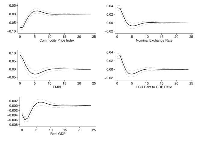
The Latin America model is estimated with two lags. Figure 2 presents the impulse response function to a one standard deviation negative shock in commodity price index cyclical

compo-nent. It is clear that when the commodity price reduces, nominal exchange rate, EMBI spreads and LCU debt to GDP ratio increase, reflecting the countercyclical relations found before. In contrast, real GDP exhibits the expected procyclical behavior. This effects are statistically

sig-nificant for around three periods (quarters).

At first sight, the magnitude of the responses might look negligible but it is worth noting that these are quarterly responses. In order to obtain a clearer response, we aggregate the quar-terly changes to get the annual (cumulative) response. In this exercise, we alter the magnitude

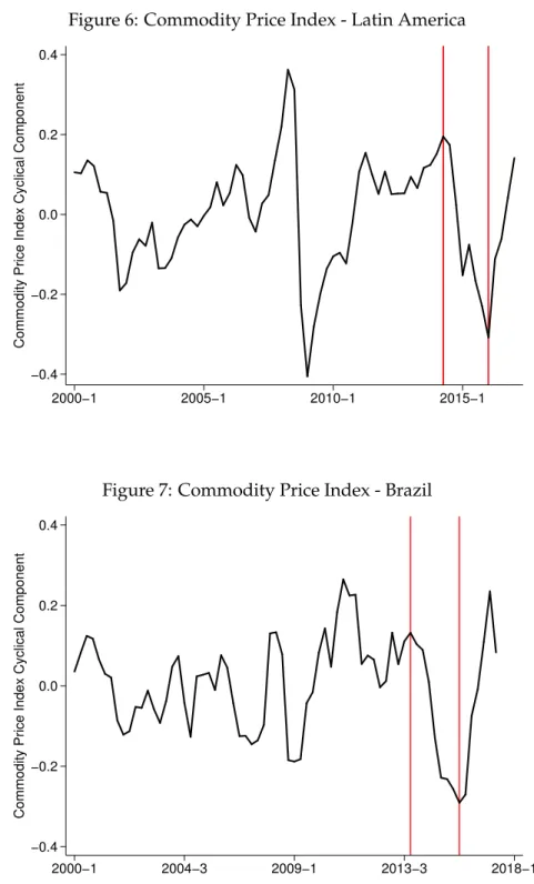
of the shock in order to capture the variation in commodity price index from boom to bust, as shown in figure 6 in Appendix A12_{These calculations are presented in table 2.}

10_{We used alternatives cycle measures, yielding no significant differences with respecto to the Hodrick-Prescott}

filter.

11_{In VAR model applications, it is usual to find confidence intervals of up to 68%. This practice became popular}

since Sims and Zha (1999) published their very influencial paper.

12_{Boom was observed in 2014}_Q_{2, corresponding to a positive deviation from its long run trend of 19.35% and bust}

(14)

Figure 2: Impulse Response Function - One standard deviation shock in commodity price index - 70% confidence intervals

−0.10 −0.05 0.00 0.05

0 5 10 15 20 25 Commodity Price Index

−0.02 0.00 0.02 0.04

0 5 10 15 20 25 Nominal Exchange Rate

−0.05 0.00 0.05 0.10

0 5 10 15 20 25 EMBI

−0.02 0.00 0.02 0.04

0 5 10 15 20 25 LCU Debt to GDP Ratio

−0.008 −0.006 −0.004 −0.002 0.000 0.002

0 5 10 15 20 25 Real GDP

Table 2: Cumulative responses - Impulse Response Function to a 2.5 standard deviation

nega-tive shock in commodity price index.

Step Nominal Exchange Rate EMBI Spread LCU Debt to GDP Ratio Real GDP

0 0.0893 0.2265 0.0771 -0.0089

1 0.0857 0.1592 0.0797 -0.0148

2 0.0444 0.0534 0.0324 -0.0131

3 0.0064 -0.0215 -0.0070 -0.0067

Cumulative

response 21.93% 38.57% 18.92% -4.35%

Table 2 shows that when commodity price index falls in almost 20% in a period, the

cumu-lative significant response in real GDP would be approximately 4.4% three periods after the shock. The effect in nominal exchange rate and LCU debt to GDP ratio are significant until two quarters after the shock, yielding cumulative changes of 22% and 19%, respectively. EMBI

(15)

Figure 3: Forecast Error Variance Decomposition - 70% confidence intervals

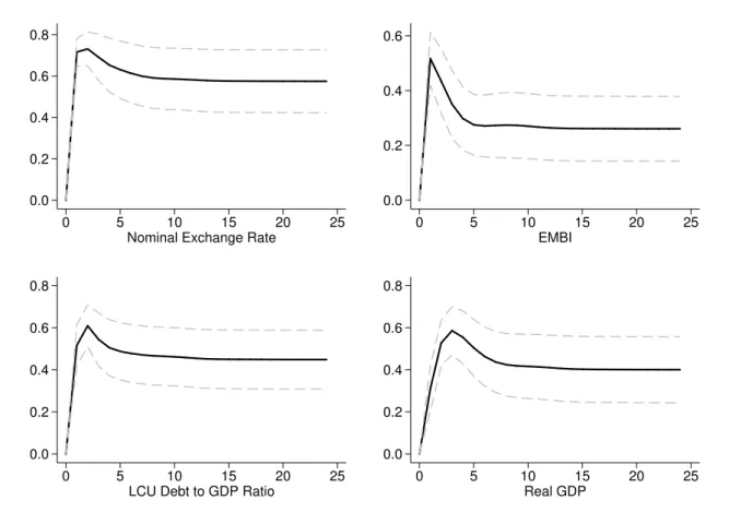
0.0 0.2 0.4 0.6 0.8

0.0 0.2 0.4 0.6

0 5 10 15 20 25 EMBI

0.0 0.2 0.4 0.6 0.8

0 5 10 15 20 25 Real GDP

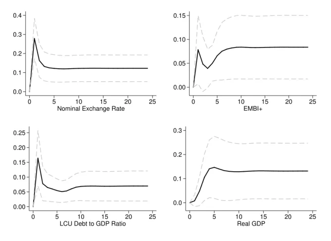
Finally, forecast error variance decomposition (FEVD) from this model is presented in

fig-ure 3. Based on this, one can conclude that around 60% of forecast error variance of nominal exchange rate is due to commodity price shocks. This proportion is approximately 30% for EMBI spread. Regarding to LCU Debt to GDP ratio and real GDP errors, it is clear that

com-modity price shocks explain roughly 40% of them.

According to these results, we conclude that commodity prices shocks do play an important role explaining the dynamics of the economic variables included, both in the region and the five

EMEs, excepting Chile. It is particularly interesting that external debt do react to changes in commodity prices. But, is this evidence enough to conclude that the balance sheet effect actu-ally exists? To answer this question, we estimate a VAR model restricting the external debt to

not respond to commodity prices shocks. The idea is to have a sort of counterfactual exercise that allows us to obtain the responses that would take place if the financial mechanism were

not relevant.

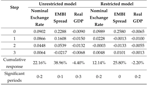
Table 3 displays the cumulative responses of the unrestricted model and the restricted

model. We compare significant cumulative responses in both models. In terms of nominal exchange rate, depreciation is 10% higher in the unrestricted model. It implies that, since

(16)

the exchange rate depreciation originally caused by commodity price fall.

Regarding EMBI spread, the unrestricted model again generates a higher response than the

restricted. This might be associated to the underlying financial accelerator. The intuition is that commodity price fall induces a first increase in EMBI spreads because economy is less attrac-tive for foreign lenders but, since entrepreneurs’ net worth is negaattrac-tively affected by the initial

shock, it provokes a further increase in risk premium.

Table 3: Impulse response function comparison: Unrestricted model vs. Restricted model -Negative shock in commodity price index of 20%

Step Unrestricted model Restricted model

Nominal

Exchange Rate

EMBI

Spread

Real

GDP

Nominal

EMBI

Spread

Real

GDP

0 0.0902 0.2288 -0.0090 0.0989 0.2580 -0.0065

1 0.0866 0.1608 -0.0150 0.0228 -0.0013 -0.0100

2 0.0448 0.0539 -0.0132 -0.0003 -0.0133 -0.0055

3 0.0064 -0.0217 -0.0068 0.0048 0.0101 -0.0013

Cumulative

response 22.16% 38.96% -4.40% 12.14% 25.80% -2.20%

Significant

periods 0-2 0-1 0-3 0-2 0 0-2

Lastly, the GDP contraction is higher in the unrestricted model. Here, again, we can

at-tribute this finding to the financial accelerator. First, the fall in commodity price reduces com-modity exports and, ceteris paribus, aggregate demand. Then, given the increase in debt

ser-vice payments, firms can not easily carry out investment projects. The increased risk premium hinders new debt acquisition to finance investment. Thus, the financial accelerator causes a

further contraction in aggregate demand and hence, in real GDP. Based on these results, we conclude that balance sheet effect does exist and it plays an important role deepening business cycles associated to commodity prices disturbances in EMEs.

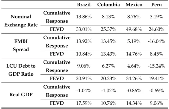
Finally, cumulative responses in impulse response functions and forecast error variance

de-composition for Brazil, Colombia, Mexico and Peru are displayed in table IV13. Since we are considering shocks of the same magnitude, these results are comparable. Brazil appears to be the most vulnerable economy to commodity prices disturbances: it has the highest increases

on exchange rate and risk premium, while having the deepest GDP contraction.

Disconcert-13_{Impulse Response Function and Forecast Error Variance Decomposition from the estimated model for each}

(17)

ingly, unlike its counterparts, in the Peruvian case, EMBI spread and LCU debt to GDP ratio

are countercyclical to commodity prices.

Table 4: Cumulative responses and Forecast Error Variance Decomposition - A one standard

deviation negative shock in country-specific commodity price.

Brazil Colombia Mexico Peru

Nominal Exchange Rate

Cumulative

Response 13.86% 8.13% 8.76% 3.19%

FEVD 33.01% 25.37% 49.68% 24.60%

EMBI Spread

Cumulative

Response 13.92% 13.45% 5.19% -16.04%

FEVD 10.84% 13.43% 14.76% 8.45%

LCU Debt to GDP Ratio

Cumulative

Response 9.06% 6.27% 4.64% -15.24%

FEVD 20.91% 20.23% 34.26% 19.41%

Real GDP

Cumulative

Response -1.04% -1.02% -0.86% -0.69%

FEVD 17.59% 10.76% 14.34% 9.06%

Chile

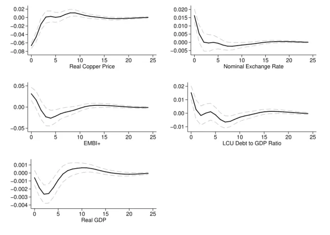
In the Chilean case, we run the model using real copper price, deflated using US consumer

price index. In this case, we estimate equation 7 withp=2. The impulse response function to a negative one standard deviation shock in real copper price is displayed in figure 4. Qualitative

behavior of endogenous variables is the same as in the region. Significance of these responses covers, at best, four quarters after the shock. For instance, the effect in nominal exchange rate, EMBI+ and LCU debt to GDP ratio is only significant on impact, after that, we can not reject

(18)

Figure 4: Impulse Response Function - One standard deviation shock in real copper price - 70% confidence intervals −0.08 −0.06 −0.04 −0.02 0.00 0.02

0 5 10 15 20 25

Real Copper Price

−0.005 0.000 0.005 0.010 0.015 0.020

0 5 10 15 20 25

Nominal Exchange Rate

−0.05 0.00 0.05

0 5 10 15 20 25

EMBI+

−0.01 0.00 0.01 0.02

0 5 10 15 20 25

LCU Debt to GDP Ratio

−0.004 −0.003 −0.002 −0.001 0.000 0.001

0 5 10 15 20 25

Real GDP

As can be seen in figure 8 in Appendix A, the last copper price fall, between periods 2014Q3

and 2016Q1 was not so prominent. In fact, from boom to bust, the copper price variated 23.48%, which in average represents a variation of 3.35% per quarter. Given this, cumulative responses

are calculated using a one standard deviation shock.

Table 5: Cumulative responses - Impulse Response Function to a one standard deviation

nega-tive shock in real copper price.

Step Nominal

Exchange Rate

EMBI Spread

LCU Debt

to GDP Ratio Real GDP

0 0.0163 0.0315 0.0153 -0.0006

1 0.0052 0.0168 0.0028 -0.0018

2 0.0001 -0.0072 -0.0017 -0.0026

3 -0.0004 -0.0231 0.0001 -0.0026

4 0.0000 -0.0263 0.0011 -0.0018

Cumulative

(19)

Table 5 displays the results of the cumulative response analysis. Since nominal exchange

rate, EMBI+ and LCU debt to GDP ratio are only significant on impact, the responses are, as can be seen in the third row of the table, 1.63%, 3.15% and 1.53%, respectively. In the case of GDP,

the cumulative response, corresponding to periods 1 to 4 after the shock is−0.89%. The Chilean case is remarkably different from its counterparts and the region. This can be attributable to the institutional structure characterizing this economy, that have allowed it to accomplish a good

credibility and reputation in the international markets. Besides, the existence of the economic and social stabilization fund (ESSF) may help to cushion the economy from the effects of copper

price volatility and hence, soften business cycles caused by it. In fact, as explained by Solimano and Calder ´on (2017), the role of the fund in dampening the effects of international copper price

volatility on Chilean economy, also brings stability to fiscal budget and policy.

0.0 0.1 0.2 0.3 0.4

0 5 10 15 20 25

0.00 0.05 0.10 0.15

0 5 10 15 20 25

EMBI+

0.00 0.05 0.10 0.15 0.20 0.25

0 5 10 15 20 25

0.0 0.1 0.2 0.3

0 5 10 15 20 25

Real GDP

Figure 5 exhibits the forecast error variance decomposition for the Chilean case. According to it, around 10% in nominal exchange rate and real GDP error variance is associated with

copper price shocks. The fraction of the error variance of both EMBI+ and LCU debt to GDP ratio explained by copper price innovations is below 10%. These are, again, timid numbers

(20)

V

Conclusions

Emerging market economies, particularly the commodity exporter ones, are exposed to world’s

dynamics through different channels. In this paper, we considered the role of (exogenous) com-modity prices shocks in explaining business cycles in EMEs. Mainstream economic literature

relates the commodity prices disturbances to business cycles through the traditional commer-cial channel, leaving behind the potential role played by financommer-cial variables.

We go further this approach by proposing a financial transmission mechanism of commod-ity prices shocks: the balance sheet effect. This effect is approached in economic literature as

being related to international interest rates shocks, without taking into account the commodity prices. We aim to connect the latter to the balance sheets of firms that possess debt denominated

in foreign currency. In this context, there is a currency mismatch between firm’s revenues and liabilities, hindering investment and hence, production when depreciation in exchange rate takes place.

Our hypothesis is that firm’s external debt dynamics are related to an exogenous

macroeco-nomic variable: commodity price. An increase in this variable reduces both nominal exchange rate and risk premium, facilitating external debt acquisition by domestic firms. But,

when-ever commodity prices fall, the opposite happens and hinders firm’s investment. In this sense, we propose that balance sheet effect acts a sort of financial accelerator that, when commodity prices are high exaggerates output’s expansion (through the increased investment), but when

commodity’s conditions are adverse, deepenes output’s contraction.

To test our hypothesis, we estimate a series of VAR models using data from Latin America and then, we focus on five particular economies: Brazil, Chile, Colombia, Mexico and Peru. We use corporate external debt, nominal exchange rate, EMBI+ spreads and real GDP data.

Besides, we construct the local currency value of external debt to nominal GDP ratio.

Our estimations allow us to conclude that Brazil, Colombia, Mexico and Peru emulate the observed qualitative behavior in the region. All variables comove as expected with

commodity-relevant price measures, i.e., nominal exchange rate, EMBI spread and the debt ratio are coun-tercyclical, while real GDP is procyclical. Chile constitutes a remarkable exception from its counterparts, where we found no evidence of copper price disturbances being a business cycle

driver. We attribute these findings to Chile’s ESSF and other institutional arrangements, such as fiscal policy rules. Moreover, in the Chilean case, the fact that this economy has the highest

external debt to GDP ratio seems not to be relevant.

(21)

be zero. By doing so, we try to answer how would the variables in the system respond if the

financial channel were not important.

Comparing impulse response functions and cumulative responses for the region and the economies (excepting Chile), we find that balance sheets do matter and they exacerbate the output’s contraction when the commodity price shock is negative. We find that, turning the

financial channel off, the real GDP cumulative response in Latin America is half smaller than in the unrestricted model. Nominal exchange rate and EMBI spread are approximately 10%

and 13% smaller, respectively. Again, Chile exhibits a different behavior from the region.

An implicit assumption we make in our paper is that companies do not cover from ex-change rate risk. This is a limitation that could be overcome in future works. It would also be important to propose a theoretical model that consideres the effects of commodity prices in

EMEs through both the traditional and financial channels. Furthermore, Structural VAR mod-els could be useful to capture contemporaneous relations between variables, which are also

(22)

Appendix A

Figure 6: Commodity Price Index - Latin America

−0.4 −0.2 0.0 0.2 0.4

Commodity Price Index Cyclical Component

2000−1 2005−1 2010−1 2015−1

Figure 7: Commodity Price Index - Brazil

−0.4 −0.2 0.0 0.2 0.4

(23)

Figure 8: Real Copper Price - Chile

−0.6 −0.4 −0.2 0.0 0.2 0.4

Real Copper Price Cyclical Component

2000−1 2004−3 2009−1 2013−3 2018−1

Figure 9: Real Oil Price - Colombia and Mexico

−0.6 −0.4 −0.2 0.0 0.2 0.4

Real Oil Price Cyclical Component

(24)

Figure 10: Commodity Price Index - Peru

−0.3 −0.2 −0.1 0.0 0.1 0.2

(25)

Appendix B: IRF and FEVD

I Impulse Response Functions

I.1 Brazil

Figure 11: Impulse Response Function - One standard deviation shock in commodity price

index - 70% confidence intervals

−0.08 −0.06 −0.04 −0.02 0.00 0.02

0 5 10 15 20 25

Commodity Price Index

0.00 0.01 0.02 0.03 0.04

0 5 10 15 20 25

−0.02 0.00 0.02 0.04 0.06

0 5 10 15 20 25

EMBI+

−0.01 0.00 0.01 0.02 0.03 0.04

0 5 10 15 20 25

−0.004 −0.002 0.000 0.002

0 5 10 15 20 25

(26)

I.2 Colombia

Figure 12: Impulse Response Function - One standard deviation shock in real oil price - 70%

confidence intervals

−0.15 −0.10 −0.05 0.00

0 5 10 15 20 25 Real Oil Price

0.00 0.01 0.02 0.03

−0.02 0.00 0.02 0.04 0.06

0 5 10 15 20 25 EMBI+

0.00 0.01 0.02 0.03 0.04

−0.0025 −0.0020 −0.0015 −0.0010 −0.0005 0.0000

(27)

I.3 Mexico

Figure 13: Impulse Response Function - One standard deviation shock in real oil price - 70%

confidence intervals

−0.15 −0.10 −0.05 0.00 0.05

0 5 10 15 20 25 Real Oil Price

−0.01 0.00 0.01 0.02 0.03

−0.05 0.00 0.05

0 5 10 15 20 25 EMBI+

−0.01 0.00 0.01 0.02 0.03

−0.004 −0.002 0.000 0.002 0.004

(28)

I.4 Peru

Figure 14: Impulse Response Function - One standard deviation shock in commodity price

index - 70% confidence intervals

−0.06 −0.04 −0.02 0.00 0.02

0 5 10 15 20 25

Commodity Price Index

−0.005 0.000 0.005 0.010

0 5 10 15 20 25

−0.04 −0.02 0.00 0.02

0 5 10 15 20 25

EMBI+

−0.04 −0.02 0.00 0.02

0 5 10 15 20 25

−0.003 −0.002 −0.001 0.000 0.001

0 5 10 15 20 25

(29)

II Forecast Error Variance Decomposition

II.1 Brazil

0.0 0.1 0.2 0.3 0.4 0.5

0 5 10 15 20 25

0.0 0.1 0.2 0.3

0 5 10 15 20 25

EMBI+

0.0 0.1 0.2 0.3 0.4

0 5 10 15 20 25

0.0 0.1 0.2 0.3

0 5 10 15 20 25

(30)

II.2 Colombia

0.0 0.1 0.2 0.3 0.4

0 5 10 15 20 25

0.00 0.05 0.10 0.15 0.20 0.25

0 5 10 15 20 25

EMBI+

0.0 0.1 0.2 0.3 0.4

0 5 10 15 20 25

0.00 0.05 0.10 0.15 0.20 0.25

0 5 10 15 20 25

(31)

II.3 Mexico

0.0 0.2 0.4 0.6 0.8

0.00 0.05 0.10 0.15 0.20 0.25

0 5 10 15 20 25 EMBI+

0.0 0.1 0.2 0.3 0.4 0.5

0.00 0.05 0.10 0.15 0.20 0.25

(32)

II.4 Peru

0.0 0.1 0.2 0.3 0.4

0 5 10 15 20 25

0.00 0.05 0.10 0.15 0.20

0 5 10 15 20 25

EMBI+

0.0 0.1 0.2 0.3

0 5 10 15 20 25

0.00 0.05 0.10 0.15 0.20

0 5 10 15 20 25

(33)

Appendix C: Estimated Balance Sheet Effects

Brazil

Table 6: Impulse response function comparison: Unrestricted model vs. Restricted model

-Negative shock in commodity price index of 20%

Step Unrestricted model Restricted model Nominal Exchange Rate EMBI Spread Real GDP Nominal Exchange Rate EMBI Spread Real GDP

0 0.0448 0.0349 0.0013 0.0729 0.0930 0.0016

1 0.0794 0.0591 -0.0068 0.0418 -0.0321 -0.0080

2 0.0815 0.0908 -0.0086 0.0217 0.0041 -0.0089

3 0.0682 0.1044 -0.0078 0.0215 0.0625 -0.0052

4 0.0521 0.1040 -0.0061 0.0246 0.0868 -0.0022

5 0.0382 0.0935 -0.0044 0.0208 0.0770 -0.0010

6 0.0270 0.0759 -0.0031 0.0123 0.0535 -0.0009

Cumulative

response 39.11% 46.87% -3.36% 21.56% 37.29% -2.22%

Significant

periods 0-6 2-6 1-5 0-6 0, 3-6 1-3

Chile

-Negative shock in real copper price of 20%

0 0.0490 0.0969 -0.0018 0.0637 0.1026 -0.0041

1 0.0153 0.0569 -0.0057 0.0152 0.0572 -0.0050

2 0.0001 -0.0138 -0.0082 0.0020 -0.0009 -0.0065

3 -0.0008 -0.0626 -0.0080 -0.0008 -0.0465 -0.0060

4 0.0006 -0.0741 -0.0058 0.0001 -0.0618 -0.0042

5 -0.0009 -0.0620 -0.0030 0.0016 -0.0525 -0.0022

6 -0.0041 -0.0465 -0.0007 0.0024 -0.0333 -0.0008

7 -0.0063 -0.0363 0.0006 0.0024 -0.0164 -0.0001

Cumulative

response 4.90% -12.19% -2.78% 7.89% -3.43% -2.80%

Significant

(34)

Colombia

-Negative shock in real oil price of 20%

0 0.0402 0.0734 -0.0014 0.0487 0.0888 -0.0014

1 0.0304 0.0643 -0.0021 0.0249 0.0543 -0.0022

2 0.0232 0.0508 -0.0025 0.0127 0.0312 -0.0024

3 0.0179 0.0367 -0.0025 0.0063 0.0151 -0.0022

4 0.0138 0.0240 -0.0024 0.0028 0.0040 -0.0018

5 0.0106 0.0139 -0.0021 0.0010 -0.0028 -0.0014

6 0.0081 0.0063 -0.0017 0.0000 -0.0064 -0.0010

7 0.0061 0.0013 -0.0014 -0.0004 -0.0077 -0.0007

8 0.0045 -0.0017 -0.0010 -0.0006 -0.0075 -0.0004

Cumulative

response 13.61% 22.51% -1.71% 9.25% 17.44% -1.11%

Significant

periods 0-5 0-3 1-8 0-3 0-2 1-6

Mexico

-Negative shock in real oil price of 20%

0 0.0254 0.0502 -0.0036 0.0303 0.0600 -0.0046

1 0.0331 0.0366 -0.0041 0.0259 0.0182 -0.0033

2 0.0313 0.0077 -0.0039 0.0202 -0.0096 -0.0021

3 0.0255 -0.0191 -0.0028 0.0151 -0.0256 -0.0011

4 0.0188 -0.0374 -0.0013 0.0110 -0.0328 -0.0002

5 0.0125 -0.0463 0.0002 0.0080 -0.0343 0.0005

6 0.0074 -0.0475 0.0014 0.0059 -0.0324 0.0010

7 0.0036 -0.0435 0.0022 0.0044 -0.0288 0.0012

8 0.0010 -0.0366 0.0026 0.0034 -0.0246 0.0013

9 -0.0006 -0.0285 0.0027 0.0027 -0.0206 0.0013

Cumulative

response 14.65% -15.29% -1.44% 12.07% -13.92% -1.01%

Significant

(35)

Peru

-Negative shock in commodity price index of 20%

Step Unrestricted model Restricted model Nominal

EMBI

Spread

Real

GDP

Nominal Exchange

Rate

EMBI

Spread

Real

GDP

0 0.0464 0.0112 0.0023 0.0843 0.0740 0.0027

1 0.0815 0.0212 -0.0056 0.0478 -0.0477 -0.0075

2 0.0850 0.0321 -0.0081 0.0281 -0.0226 -0.0084

3 0.0735 0.0391 -0.0088 0.0261 0.0078 -0.0063

4 0.0586 0.0394 -0.0079 0.0248 0.0149 -0.0038

5 0.0453 0.0335 -0.0063 0.0188 0.0073 -0.0019

6 0.0338 0.0231 -0.0045 0.0110 -0.0009 -0.0007

Cumulative

response 42.41% NA -4.12% 24.09% 7.40% -2.59%

Significant

(36)

References

Benavente, J. M., Johnson, C. A., and Morande, F. G. (2003). Debt composition and balance

sheet effects of exchange rate depreciations: a firm-level analysis for chile. Emerging Markets Review, 4(4):397–416.

Bernanke, B. S., Gertler, M., and Gilchrist, S. (1999). The financial accelerator in a quantitative

business cycle framework.Handbook of macroeconomics, 1:1341–1393.

Bonomo, M., Martins, B., and Pinto, R. (2003). Debt composition and exchange rate balance

sheet effect in brazil: a firm level analysis.Emerging Markets Review, 4(4):368–396.

Carranza, L. J., Cayo, J. M., and Gald ´on-S´anchez, J. E. (2003). Exchange rate volatility and economic performance in peru: a firm level analysis. Emerging Markets Review, 4(4):472–496.

C´espedes, L. F., Chang, R., and Velasco, A. (2004). Balance sheets and exchange rate policy. American Economic Review, 94(4):1183–1193.

Charnavoki, V. (2010). Commodity price shocks and real business cycles in a small

commodity-exporting economy.

Echeverry, J. C., Fergusson, L., Steiner, R., and Aguilar, C. (2003). ‘dollar’debt in colombian firms: are sinners punished during devaluations? Emerging Markets Review, 4(4):417–449.

Fern´andez, A., Gonz´alez, A., and Rodriguez, D. (2017a). Sharing a ride on the commodities roller coaster: common factors in business cycles of emerging economies. Journal of

Interna-tional Economics.

Fern´andez, A., Schmitt-Groh´e, S., and Uribe, M. (2017b). World shocks, world prices, and business cycles: An empirical investigation. Journal of International Economics, 108:S2–S14.

Gertler, M., Gilchrist, S., and Natalucci, F. M. (2007). External constraints on monetary policy and the financial accelerator. Journal of Money, Credit and Banking, 39(2-3):295–330.

Gruss, B. (2014). After the boom–commodity prices and economic growth in Latin America and the Caribbean. Number 14-154. International Monetary Fund.

Kose, M. A. (2002). Explaining business cycles in small open economies:‘how much do world

prices matter?’.Journal of International Economics, 56(2):299–327.

Lobato, I., Pratap, S., and Somuano, A. (2003). Debt composition and balance sheet effects of exchange rate volatility in mexico: a firm level analysis. Emerging Markets Review, 4(4):450–

471.

Malone, S. (2009). Balance sheet effects, external volatility, and emerging market spreads.

(37)

Mendoza, E. G. (1995). The terms of trade, the real exchange rate, and economic fluctuations.

International Economic Review, pages 101–137.

Reinhart, C. M., Reinhart, V., and Trebesch, C. (2016). Global cycles: Capital flows, commodi-ties, and sovereign defaults, 1815–2015.The American Economic Review, 106(5):574–580.

Shousha, S. (2016). Macroeconomic effects of commodity booms and busts: The role of financial frictions.Unpublished Manuscript.

Sims, C. A. and Zha, T. (1999). Error bands for impulse responses. Econometrica, 67(5):1113–

1155.

Sinnott, E., Nash, J., and De la Torre, A. (2010). Natural resources in Latin America and the

Caribbean: beyond booms and busts? World Bank Publications.

Solimano, A. and Calder ´on, D. (2017). The copper sector, fiscal rules, and stabilization funds in chile: Scope and limits. Technical report, WIDER Working Paper.

Tretvoll, H., Leibovici, F., and Kohn, D. (2017). Trade in Commodities and Emerging Market Business Cycles. Technical report.

Vegh, C., Morano, L., and Friedheim, D. (2017). LAC Semiannual Report October 2017: Between