Resumen:
El presente estudio analiza el impacto de las variaciones en el precio de las materias primas en el desempeño macroeconómico y en la política fiscal de ocho países de América Latina (AL) en el período 1998-2014. En particular, se analiza la relación existente entre las variaciones de precios en los commodities con los ciclos económicos que experimentan los países de la región y el canal de transmisión existente entre la política fiscal y el crecimiento económico. Para analizar estas variaciones, se construyó un índice de precios de las materias primas para cada país, basado en la metodología de Medina (2010). Para estimar el impacto de un shock en los precios, se estimó un modelo de Vectores Autorregresivos con datos de panel utilizando la descomposición de Cholesky. La reacción de las variables macroeconómicas y fiscales es también comparada con la respuesta de un conjunto de países desarrollados exportadores de materias primas. Los resultados del modelo indican que las fluctuaciones de los precios de las materias primas es un factor potencial de inestabilidad en el crecimiento económico de los países latinoamericanos así como de los países de altos ingresos exportadores de materias primas, aunque la magnitud y el canal de propagación de los choques tienden a ser mucho más altos en los países de AL. En la misma línea se identificó que existe una fuerte dependencia de los ingresos fiscales a las fluctuaciones de los precios de las materias primas para los dos grupos de países, no obstante la respuesta del gasto
ASSESSING THE EFFECT OF COMMODITY PRICE SHOCKS IN THE MACROECONOMIC PERFORMANCE AND FISCAL OUTCOMES IN LATIN AMERICA
COUNTRIES
Luis Alberto Páez Vallejo*
* Economista de la Pontifica Universidad Católica del Ecuador, Máster en Economía Aplicada por la Universidad Paris X (Francia). Funcionario de la Dirección Nacional de Riesgo Sistémico del Banco Central del Ecuador. Email: [email protected].
Las opiniones vertidas en este documento son de responsabilidad exclusiva del autor y no repre- sentan la posición oficial del Banco Central del Ecuador ni de sus autoridades.
Los Anexos de este articulo pueden ser solicitados al correo electrónico del autor.
público tiende a ser más procíclica en el caso de los países de AL, mientras que para los países desarrollados, la reacción de la política fiscal es anticíclica. Este resultado respaldaría la idea de que la política fiscal en los países de AL es un factor potencial que amplifica el mecanismo de transmisión de la volatilidad inherente en los precios de los commodities a los agregados macroeconómicos.
Palabras clave: Crecimiento económico, Commodities, PVAR, Política Fiscal Contracíclica, América Latina.
Clasificación JEL: O4, Q11, C3, E62, H62, N16 Abstract:
In this study we investigate the role of commodity price shocks in the macroeconomic performance and in fiscal outcomes in eight Latin American (LA) economies during the period 1998-2014. Particularly, we assess the role of the commodity cycles in driving the business cycle in LA economies and how it influences also the adjustment of the fiscal policy. To do it, we constructed a specific commodity index for each country based in Medina methodology (2010). To exploit this relationship, we analyzed the effect of index commodity prices shocks using a Panel Vector Auto Regression methodology (PVAR) and using the Cholesky identification. The macroeconomic effects and fiscal reactions of LA countries are compared with a set of high income commodity exporting countries. The results of the PVAR methodology indicate that commodity cycles is a potential cause of economic cycles in LA countries, and that the magnitude of the effect is more important in LA countries compared to high income commodity countries. In the same line, evaluating the direct effect of the commodity shock in primary expenditure, we found that in LA countries the fiscal policy is procyclical while high income commodity countries, despite having a significant impact on their fiscal incomes- windfall revenues, they show a counter cyclical fiscal policy. This result supports the idea that the fiscal policy in LA countries can be a potential factor that can amplify the transmission mechanism of the inherent volatility of commodity prices to macroeconomic aggregates.
Keywords: GDP growth, Commodity, PVAR, Counter cyclical Fiscal Policy, Latin America.
JEL Classification: O4, Q11, C3, E62, H62, N16
I. INTRODUCTION
A large number of studies have investigated the transmission channels in which the commodity price fluctuations have an impact on economic activity, focusing in particular on the response of economic growth and consumer price inflation.
One of the most important studies in this literature is Bruno and Sachs (1985), who were the firsts to analyze the macroeconomic effect of oil prices on output and inflation in the major industrialized countries during the 1970´s. More specifically, some studies as the one presented by Hamilton (1985), focused in the effect of oil shocks in US economy. Among its most significant findings he showed that most of U.S recessions were preceded by increases in the oil price, suggesting the essential role of oil price increases as one of the main causes of recessions. Few years later, these results were invalidated by Hooker (1996) whose principal findings suggested that the linear relationship between oil prices and output fluctuations was inconsistent after 1973.
In relation to this long debate, Blanchard and Galí (2007) discussed the macroeconomic effect of oil prices in different episodes, differentiating the oil price shock of the 70´s with the one experimented during the 2000´s. Their main results are that, the effects of a given variation in oil prices have changed substantially over time, the larger effects on inflation and economy activity where found in the first episodes in the 70´s, and after this period the effect has been muted over time.
However, most of these studies have focused on the impact of oil price shocks in developed countries such as the US or European countries (which in generally tend to be oil importing countries) and few studies have examined the effects of commodity price shocks in low or middle income commodity exporting countries.
In the group of studies that considers not just the oil price shock but a set of primary commodity prices and evaluates their effect in macroeconomic aggregates in low income exporter countries, we can find for example the study of Deaton and Miller (1995). They assess the impact of commodity prices shocks on Sub Sahara African countries and analyze whether poor macroeconomic results can be more attributed to the difficulty of these economies to predict commodity prices fluctuations or to create endogenous mechanisms to protect their economies from these external shocks. In relation to the mechanisms channels that the commodity shocks can affect the macroeconomic performance in emerging economies, in the literature we can found three main channels:
First, a positive shock of commodity prices, generates incomes windfall that come from the performance of the commodity exporting sectors due to a favorable terms of trade effect that has the potential to affect the entire aggregate economy (spillover effect). For instance, higher incomes in the economy increase domestic aggregate demand and thereby stimulate the domestic output. Following Da Silva (2011), the extent of this effect depends on the degree of interaction with other sectors, in the degree of diversification of their productive sector.
Second, if a country is a net importer of a specific commodity as oil, a positive shock in commodity prices can also have the potential effect to reduce the level of output through a negative supply effect. For example, considering the case of a net oil importer country, a higher increase in the oil prices produces a negative supply effect (as is commonly evaluated in the literature), because as being the oil an important input in firm productions, in largely all the sectors of an economy, an increase in the price will lead to an increase in the production cost, what consequently produces a reduction of potential output (reduces productivity) and increases the domestic prices.
Third, concerning the policy framework that can help to amplify or mitigate the commodity shock, authors as Aslam, Strom, Bems, Celasun (2016) have also noted that the reaction of fiscal policy to higher commodity revenues can also be a potential additional factor that affects the transmission channel.
However, there exist few studies in the literature that have explored in particular this relation between the impact of commodity prices in macroeconomic aggregates as well on fiscal outcomes.
Among the principal researches that concentrated their analysis on fiscal policy reactions to external adverse shocks in low income countries, Boccara (1994) suggests that typically when the government expenditure rises during the boom cycle, once the boom has ended, it is very difficult for governments to adjust them.
The author suggests that this difficulty can be explained by three main factors: the existence of a pressure to spend, because there are a lot of unmet needs, special interest groups or internal government pressure which produces a political economy cost.1
1 Also it could be by a limited disinvestment, as for example in investment spending in large projects or the size of the public force, where the government is trapped by a recurrent and inflexible expenditure or even irreversible.
There are also some studies that tend to link commodity prices shocks and GDP fluctuations, and their effects by an indirect approach in fiscal outcomes in Latin American (LA) countries. Gavin and Perotti (1997) identified that fiscal policy in these countries tend to be procyclical, even more in periods of low growth. More recently, Ilzetsky and Vegh (2008) using a large set of econometric tests (instrumental variables, simultaneous equations, times series methods) have similar conclusions, fiscal policy is procyclical and is expansionary.
As Medina (2011) suggests, typically all these studies focused on documenting the fiscal reaction to the economic cycle only in an indirect way (they linked the effect of commodity prices fluctuations with the fiscal results only through the channel of GDP fluctuations). In the same way, in order to evaluate the cyclicality of fiscal variables, a lot of studies use government consumption or overall fiscal balances.
While for the first variable specification, the fiscal reaction is underestimated because the public investment is missed (which is a large part of public spending), for the second specification, the overall balance is an adjusted variable that already considers the procyclical performance of revenues and spending, for instance it is difficult that this latter can potentially measure the direct impact of an external shock.
Considering all the literature discussed above, this study focuses in understanding the direct impact of commodity prices fluctuations on fiscal outcomes but also in macroeconomic performance in eight LA countries from 1998 to 2014.
To exploit this relationship, as Medina’s (2010) study, we analyzed the effect of index commodity prices shocks using a Panel Vector Autoregression methodology (PVAR) and using the Cholesky identification. The macroeconomic performance and fiscal reaction of LA countries are also compared with a set of high income commodity exporting countries. In order to avoid a wrong specification of fiscal variables, we consider the total primary public expenditure instead of using overall fiscal balances or the public consumption.
We also take some distance in relation to Medina’s methodology (2010) because we constructed a much simpler index of commodity prices (assuming constant weights). In the same way, we exploited the unobservable characteristics of each country and the heterogeneity of the economies within the region, in order to construct a panel VAR model.
The structure of this study is organized as follows: The next section, analyzes general facts about the evolution of the commodity prices in the last decade and its relation with the macroeconomic performance of the LA countries. The third
section discusses the methodologies that allow us to evaluate the responses of the macroeconomic aggregates and fiscal outcomes when we simulated a positive shock in the commodity prices. The last one concludes and presents also some limitations of our methodological approach.
II. GENERAL FACTS
2.1 Commodity prices cycles and LA macroeconomic performance The unprecedented commodity boom faced by LA countries in the period 2003-2008 coincided with two main factors: a positive cycle in world financial markets that allowed LA economies to receive exceptional external financing, and a sustained increase of commodity prices until 2008 (a positive term of trade shock).
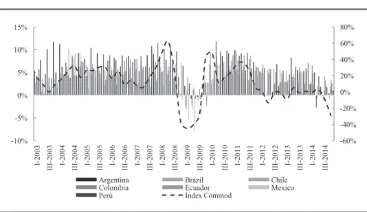
The graph 1 shows the strong relation between the annual growth rate of the commodity price index and LA economic growth. For example, from I-2003 to II- 2008, we can see that the index follows a positive growth, with an annual average growth of 20% approximately.
During the same period, the seven economies followed a positive cycle of sustained growth driven by higher disposable income revenues that stimulates the different components of the aggregate demand in terms of higher levels of private consumption, investment and public spending.
The decrease of the commodity prices once the financial crises emerged in the last quarter of 2008, have a direct impact in LA macroeconomic performance.
In the first quarter of 2009, there are only three LA economies that experimented a decrease in annual GDP growth, while for the third one, almost all registered negative growths (with the exception of Colombia). In the last quarter, there is an important recovery of the economic growth of the region that is driven largely by a retrieval of the commodity price index.
This new positive cycle of high growth in commodities prices is short and is more intensive during the period 2010-2012. In relation to this favorable environment, some LA economies experimented higher growth rates, specifically Peru, Ecuador, Chile and Argentina economies.
However, since 2013 the index began to slow down and recorded even some negative values, and with more intensity in the last semester of 2014, reaching a negative rate of 29% in the last quarter.
Graph 1: Annual GDP growth by country versus annual growth of the all commodity price index
-60%
-40%
-20%
0%
20%
40%
60%
80%
-10%
-5%
0%
5%
10%
15%
I-2003 III-2003 I-2004 III-2004 I-2005 III-2005 I-2006 III-2006 I-2007 III-2007 I-2008 III-2008 I-2009 III-2009 I-2010 III-2010 I-2011 III-2011 I-2012 III-2012 I-2013 III-2013 I-2014 III-2014
Argentina Brazil Chile
Colombia Ecuador Mexico
Perú Index Commod
Source: International Monetary Fund, Economic Commission for Latin America and the Caribbean.
This pattern affects also GDP performance in LA countries. As we can see in the graph 1, since 2013 the GDP of LA is still positive but the growth rates began to decelerate progressively, as the recessive cycle of the commodity prices is intensified.
2.2 Reprimarization symptom
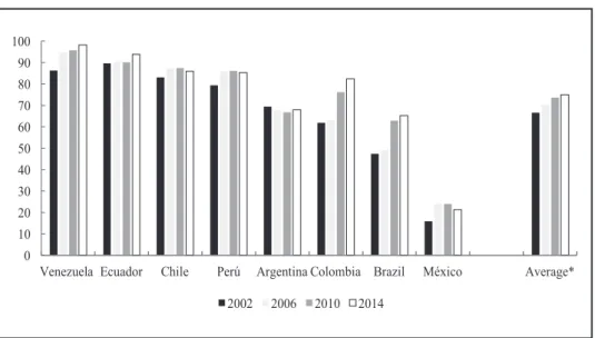
In first term, as Quenan and Velut (2014) remarked, the commodity boom of the eight LA economies is reflected by a “reprimarization symptom in their productive sectors”, especially in the agricultural sector and in primary extractive industries (see graph 2).
As we can see, in average, LA economies have done too little to diversify their economies, even more there is a potential tendency that their export sector have been more concentrated in primary products from 2002 to 2014. Actually, in average, in 2002 primary products represented about 67% of total exports value, while in 2014 they represented approximately 75%.
Among the economies in which their export concentration ratio is above the average we found for example Venezuela, where its export sector depends approximately 98% of primary product revenues, Ecuador and Chile depend in
about 93% and 85%, respectively. On the other hand, between the economies that have realized a major effort in diversifying their economies, we find for example Mexico, in which the primary products represent about 21% of total exports values in 2014. Actually, Mexico seems to be the outlier in the region. Brazil is the second one that tends to have a more diversified export sector.
Graph 2: Percentage of primary products in the total value of exports
0 10 20 30 40 50 60 70 80 90 100
Venezuela Ecuador Chile Perú Argentina Colombia Brazil México Average*
2002 2006 2010 2014
Source: Economic Commission for Latin America and the Caribbean.
This reprimarization symptom is critical because it generates an unbalanced growth and tends to slower the long term growth.
Commodity cycles and macroeconomic policies
Another important feature is to understand, giving the primary export structure and the macroeconomic policies adopted for each economy, how we can link the economic activity of LA region in the last years with the price commodity cycles.
Following Ocampo (2007), since 2000´s, after the different economic crises that emerged in the region, LA economies have implemented structural reforms in fiscal policies also in the way of managing the monetary policy and exchange rate markets. Nevertheless the opening of the capital account and a major integration of the financial markets have reduced the capacity of these economies to control the
monetary policy and the exchange autonomously.2 For instance, the only instrument policy in which LA economies have faced and can dispose autonomously is the fiscal policy.
In graph 3, we analyzed the annual average growth of some fiscal variables in relation with the commodity boom cycles, as also others variables of the external and real sector in the period 2003-2014.
Graph 3: Macroeconomic performance of the 8 LA economies (Mean value by periods)
-10%
0%
10%
20%
30%
40%
50%
CPI growth GDP growth Rev growth Expend.
growth % debt/GDP % overal
balance % current balance
2003-2008 2009 2010-2014
Source: Economic Commission for Latin America and the Caribbean.
The graph shows an important procyclicality of specific macroeconomic variables. As we already noted, during the boom cycle, the increases in terms of trade, rises the disposable revenues of household and firms, this contributes to stimulate the levels of private and public consumption, the level of investments and gives a high performance in private sector balances. This is the fundamental reason for having a higher average growth of GDP during the first period compared to other periods in the eight LA economies.
2 As for example, during the boom cycle, the monetary authority can be limited in implementing a countercyclical monetary policy (for example, an increase in interest rates) because the pressure of the external capitals, and if the government tend to avoid an appreciation in exchange rate.
In the same way, since some economies emerged from their worst economic crises (as in Argentina in 2002 and Ecuador in 1999-2000) and more general, from a decade of high macroeconomic instability (lost decade of the 90´s), this historical boom coincides also with the application of some structural reforms in their economies.
As a result, the macroeconomic performance during the boom, allowed these economies to reduce continuously the levels of inflation and the level of their public debt (see graph 3).
The favorable external conditions generated in average a positive balance in external sector from 2003 to 2008 compared with the other periods. The current account balance passed from a surplus in 2003-2008 of about 1.8% in relation with GDP to a surplus of 0.1% during the financial crises and to a deficit of -1.5% in the last five years.
The fiscal balances followed the same procyclicality behavior, the boom cycle generates buoyant fiscal resources during the first period, with more intensity in energy (oil sector) and metal exporter countries (copper sector). Actually, in this period, energy and metal exporter countries faced the largest volatilities in public revenues during the boom and the bust, because governments participate directly in the rent of oil sector and in copper (in terms of production or in royalties). In the first period, the average growth of total public revenues was about 21.3% versus -3.7% in the financial crises period and 15.5% in the last period (with a difference for about 5.5 points).
The primary public expenditure followed the same pattern but with less intensity, especially compared to the last period (2010-2014) in which the commodity prices tend to slow down. Actually, the public expenditure grew on average at a slower pace during this period (17% versus 20% respectively), but the magnitude of the reduction was proportionally less strong than the sharp slowdown in government revenues. Actually, it seems that in the lasts years, all LA economies apply a more procyclical behavior in fiscal policy compared to the first period.
In fact, while during the boom, there were only two economies -Ecuador and Venezuela- that expanded more than proportionally the primary expenditure in relation with the fiscal revenues; in the last period, almost all the economies in the region increased more the primary expenditure. In the same way, new governments appears in the political scenario (as Rafael Correa in Ecuador and Cristina Fernández
de Kirchner in Argentina, both governments assume the presidency in 2007), and reconvert their macroeconomic policies with a major presence of the public sector in the economic activity and not just as a regulatory role.
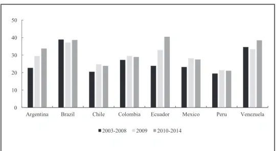
The graph 4, shows how the presence of the total public expenditure in economic activity has increased during the last years compared to the boom cycle, the public expenditure represents about 32% of the GDP in the last period whereas in the boom period it was approximately 26%.
Graph 4: Total Public Expenditure as a percentage of nominal GDP
0 10 20 30 40 50
Argentina Brazil Chile Colombia Ecuador Mexico Peru Venezuela 2003-2008 2009 2010-2014
Source: International Monetary Fund.
Indeed, the fundamental reasons of why some governments of the region didn’t adjust the public expenditure in the same dimension as revenues during these periods, can be explained by the political and social high cost of adjusting public expenditure, see (Boccara, 1994) and also by the idea that LA countries possess a relative easy access to external fundings, specially with a strategic partner that funded the region after the financial crises (China).
The result of this new panorama in the region during the period 2010-2014, is a sharp decline in fiscal buffers, a deteriorated external and fiscal balances and largest increases (at least during the 2000´s) of the public expenditure.
III. PANEL VAR METHODOLOGY 3.1 General approach
In order to evaluate the sensitivity of the macro fundamental variables and fiscal balances to commodities price changes, in this study we will use a structural panel vector autoregressive model (PVAR model). The panel VAR model combines two factors: in one hand, it combines the traditional VAR approach, that allows us to deal with the potential endogeneity issues that usually exist in macroeconomic models, treating all variables as endogenous, and on the other hand, panel data approach allow us to consider specific unobserved characteristics of each LA country.3
The reduced form of the panel VAR model can be written as follows:
(1)
Where is the vector of endogenous variables (ΔINDCOMit, ΔGDPit, ΔREVit, ΔEXPit, ΔCPIit) for country i in the quarterly t, is the vector of intercepts, is the coefficient matrix of the lagged variables p, denotes time invariant fixed effects and is the vector of innovations, which are assumed to be uncorrelated across i and t.
Since the fixed effects are supposed to be correlated with the dependent variables, one way to deal with the potential problem of endogeneity between variables is to transform the model in first differences or to consider the time demeaned approach.
Nevertheless, because VAR methodology deals in its structure with lagged dependent variables as regressors, the mean differencing procedure or the first difference methodology would create biased coefficients. To avoid this problem, Anderson and Hsiao (1982), Arellano and Bond (1991) propose the estimation of models with predetermined but not exogenous variables by implementing a two stage least square method (2SLS) using lagged variables of the predetermined variables as instruments for the equation only in first differences (Arellano and Bover (1995), p2). Nevertheless, regardless the robustness of this methodology, as Kohn (2013)
3 Causal endogeneity like for example the common relationship between GDP and fiscal variables, due to the reverse causality of these two variables.
affirms, the first differenced approach has the problem that it will magnify gaps in unbalanced panels. For instance, if yi, is missing in the data, then Δyi, and Δyi,t-1 are also missing in the transformed data.
Another useful alternative is proposed by Arellano and Bover (1995) using the Helmert´s Tranformation. This procedure, as the time demeaning procedure, subtract to each of the first observation, the mean of the remaining future observations available in the sample (Arellano, Bover, 1995, p13). For instance, the Helmert procedure subtracts the average of all the future observations and thus preserves the sample size in panels with gaps.
As Arellano and Bover (1995) explain in his study, it is possible to detail this transformation, as follows:
(2)
Where it denotes the means obtained from the future values of yi. An example of the transformed variable can be written as:
(3)
And is the weight used to equalize variances. The final PVAR model transformed takes the form as:
(4)
This transformation allows us to preserve the orthogonality between the transformed variables and the lagged regressors. Since, in the transformed model, we did not use the lagged observations for the different equations in levels, we can use them as instruments to estimate the GMM estimators.4
4 The panel VAR estimation in this paper is obtained using the Stata codes pvar developed by Inessa Love (2006). The standard procedure of estimation that I considered in this study is the same as the Love and Zicchino (2006). Therefore the model I considered is “just identified” (the number of regressors will equal the number of instruments), allowing that the system GMM has numerically equivalent to the equation-by-equation 2SLS (which is more simple and avoid using the weight matrix that is typically used in the GMM estimations).
In a panel VAR context, as the traditional VAR approach, they have the desirable property of focusing on the dynamic impact of different shocks. In order to exploit this property, as Medina suggests, (2010), it is important to first identify the relevant shock and then, the response of the system to shocks is described through the impulse response function methodology.
In this study, the main interest is to estimate the effect of the commodity prices shocks in the macroeconomic performance and fiscal outcomes of eight Latin American countries, and compare these results as Medina did (2010), with the response of three high income commodity-exporting countries.
To do this, we can simplify the notation of equation (4) and using the lag operator , we can express the reduction form of the panel VAR as follows:
(5)
The impulse response function can be computed once we invert the AR representation form to an infinite vector moving average (MA) and once we already test that the eigenvalues of the matrix are less than 1, satisfying the stability condition.
Since the innovations can be correlated contemporaneously, if we apply a specific shock to one variable -as in our case to the commodity prices index- it is likely to be accompanied by the shocks of another variables. In order to avoid this, we imposed orthogonality conditions to the innovations using as identification strategy, the Cholesky decomposition proposed by Sims (1980).
To do that, the ordering that we applied in this study followed the Medina study (2010) strategy: the country specific commodity index is ordered first, under the assumption that domestic variables as GDP, or fiscal variables or CPI index do not have a contemporaneous influence on commodity prices. This assumption can be reasonable because in this study we considered only Latin America countries which are traditionally small countries and do not have a direct influence in commodities world prices (they are price takers).
In the second position, we defined the GDP growth, by the fact that a large part of the literature in LA countries (see section I) claims that fiscal policy in LA is procyclical which implies that GDP fluctuations generate changes in fiscal
balances. In the third and fourth positions, after the GDP growth, we defined the fiscal variables -the total revenues of the government first and then the primary public expenditure-. In the last position we defined the CPI index, which depend by definition in the past values of all the variables defined previously -INDCOM,GDP, REV, EXP-. The last four variables are by definition contemporaneously affected by changes in the commodity prices.
As Medina (2010) commented, this ordering is consistent with the literature because it highlights the following mechanisms: the effects of how an external shock can affect macroeconomic aggregates, in how the fiscal policy is affected by changes in the business cycles (measure by the GDP fluctuations), the common nexus between public revenues and expenditures, also the response in domestic prices by the shocks of external prices and by changes in domestic conditions.
3.2 Sources of Data
In order to evaluate the effect of the commodity prices fluctuations on macroeconomic performance and fiscal balances, we used a quarterly data beginning as early as the first quarter of 1998 and end in the last quarter of 2014. The group of endogenous variables considered in the model is: a country specific commodity prices index (INDCOM), which is constructed for each country following Medina (2010) methodology. The real growth of Gross Domestic Product (GDP), the real growth of revenues and primary expenditure of the central government (REV and EXP) and finally the index of consumer prices (CPI).
Following Medina methodology (2010), the country specific commodity prices index (INDCOM) was constructed as follow: First, we collected the monthly historical information of the 5 main categories of the index primary commodity prices that are constructed by the IMF.5 These categories combine international historical prices of 55 commodities products. Once the data base is collected, we repeated the same index value for each sub category.6 We did this in order to link this matrix of index commodity prices with the weight values of commodity exports constructed by Medina in 2010 for eight LA countries and four developed countries.
His matrix takes into account the weights values of 52 products that represent actually between 80% or 90% of a given country’s total commodity exports in 2005.
5 Food price index, beverage price index, agricultural raw materials index, metals price index and Fuel Energy index.
6 As for example, for the historical index value of energy prices, I replicated the same value for the natural gas, coal and crude oil.
This study differs from his approach because we considered as hypothesis that these weights (that are constructed for 2005) are constant in all the periods, as in the study of Deaton and Miller (1995). Despite this restriction, the price index that we considered is important because it takes into account the different structure for each country of commodity exports, making for example countries as Ecuador or Venezuela more sensitive to the fluctuations of energy prices, or Argentina more sensitive to agricultural prices, instead of using the same index value for all the countries.
The sample includes the eight largest LA commodity exporting countries that represent in average 92% of LA GDP from 1998 to 2014. As in Medina study (2010), we decided to include three high income commodity exporting countries -Australia, Canada and Norway- in order to compare their different reactions to price commodity shocks and in this way, evaluate whether or not LA countries are more vulnerable to external shocks.
3.3 Unit root test
In order to work with vector autoregressive models, the data series need to be stationary. To test the presence of a unit root in the series, we apply two specific methodologies. First, we proceed with an individual standard unit root test apply to each variable (Augmented Dickey Fuller, Phillips-Perron and Kwiatkowski tests).
For the individual tests, the results of applying a sequential testing strategy are presented in table 1.7 In one hand, with all the series in level form, we can see, that the country specific commodity prices index is the only variable which appears to be non-stationary for all countries, in which the tendency and the constants are not significant (group of variables in which we apply the first difference filter in order to transform them to a stationary process). The results are closely the same for the CPI index and GDP growth with some exceptions in Brazil, Argentina, Colombia, Ecuador and Mexico series.8 The results of nonstationarity are corroborated by a graphical representation of the series in level form.9
7 We take a risk of critical value of 5%, but the results are the same for a risk of 1%.
8 As in difference with the index of commodities, the GDP series are stationary of order one around a constant.
9 The graphic representations of these series in logarithm form can be requested to the author at his email.
In the other hand, the fiscal variables -total revenues and the primary expenditures- present different results. The series of the total revenues of the central government of Australia, Brazil, Colombia, Ecuador and Mexico, seem to be stationary but around a deterministic trend process. For the primary expenditure variables, the results are almost the same for the latter group of countries, but including also the series of Norway and Peru.10
Verbeek (2004, p.279) noted that when a variable followed a nonstationary process, it can be caused because this variable is may be affected by the presence of a strong deterministic trend process, rather than the presence of a unit root process, or maybe both.
This could be a potential explanation of why in Augmented Dickey Fuller (ADF) and Phillips-Perron (PP) tests, the results of stationarity change radically when we decided to include or not the tendency in the group of the variables mentioned above.
One interesting and alternative methodology to transform a nonstationary variable with a deterministic trend process into a stationary process, is to remove the trend by regressing these group of variables upon a constant and a lineal trend variable, and then, considering just the residuals of this lineal regressions. Once the time trend is removed, there exist a more realistic consensus results between the three different tests. In general, we found that all these series seem to be stationary in levels, but in this case without a constant and tendency as it was expected.
Concerning these different restrictions and in order to have a more homogenous structure between all the variables, we decided finally to apply the first difference filter to all the variables of the model. The graphical representations and the results of the three tests applied to the variables in first difference form, allow us finally to conclude more consistently that they are following a stationary process.11
10 For the other countries, the fiscal variables are stationary but in first difference without a constant and tendency, what allowed us to conclude that they are integrated of order one.
11 Applying the sequential testing strategy to all the variables, we found also some exceptions. In ADF tests, we found that applying the first differences filter in the CPI of Venezuela, we fail to reject the null hypothesis that there exists the presence of a unit root process, while in the two other tests, we reject the null hypothesis but the tendency and the constant are significant, even taking a risk of 1%. In the same line, the KPSS results, shows also that almost all the variables of Ecuador in first differences, are stationary around a trend and a constant.
We also implemented a panel unit root test. The principal advantage of using panel tests, as Mignon and Lescaroux (2008) justified is that they increase the extension of data by including more information from various countries, and for instance raise the power of the standard unit root tests in finite samples. The panel tests are applied to all the variables of the model (that included also the transformed detrended variables). In general, we found approximately the same results as the standard unit root tests. In all the cases, when the series are in logarithmic first differences, the null hypothesis is rejected (taking a risk of 1%) and allow us to conclude that they can be treated as integrated of order one.
For instance, in the PVAR we are going to work with all the variables in first difference form. The optimal lag order for GMM models were defined using the MAIC criteria (the optimal lag structure was defined only in one lag).
IV. RESULTS
4.1 Granger Causality
Before analyzing the results of the PVAR model and in order to investigate the short term links between the commodity prices and the other variables, we proceed to apply a Granger causality test. Since the series are integrated in order one, the test is applied to series in first differences.
According to the results, the direction of the Granger causality generally runs from the commodity prices index to the other variables for the two groups of countries (LA economies and high income commodity countries)
With respect to LA countries, there is a Granger causality (we fail to reject the null hypothesis in 1%) from the index commodity prices to real GDP growth and fiscal outcomes in terms of government’s revenues and primary expenditures growths (these results are statistically significant even taking a risk of 1%).
Interestingly, we did not find a granger causality relation from the index commodity prices to the CPI index.
We found a Granger causality relationship that comes from the GDP to the primary expenditure; this may suggest a close relationship between the business cycle and the behavior of the public expenditure in LA economies. In the same line, we found a Granger causality relationship that comes from the public expenditure to the CPI index, this suggests that a more expansionary fiscal policy can affect domestic prices through the stimulus that it generates in domestic demand. Similarly,
the reversal relationship is also significant, the Granger causality relationship comes also from the CPI index to the public expenditure.
With respect to high income countries, there exists a Granger causality from the index commodity prices to real GDP growth, fiscal outcomes and also in the CPI index. For the last variable, this result may suggest that commodity prices can drive some variations in domestic average inflation in high income commodity countries (second round effect).
In difference with LA economies, there did not exist a Granger causality that came from GDP to primary expenditure or from primary expenditure to CPI.
4.2 Impulse response function
In order to analyze the effect of commodity price shocks in the macroeconomic performance of eight LA countries we used the impulse response function and the variance decomposition analysis. We compare the results with the response of three high income commodity export countries -Australia, Canada and Norway-.
The temporality used in the analysis is 20 quarters (five years) and the confidence intervals are constructed using a Monte Carlo simulation with 200 repetitions.
When the price shock is computed in the PVAR model, the size of one standard deviation shock in LA countries is very similar to the high income commodity export countries, in average for about 4.8% and 4.7%, respectively.
The results shows that for both, LA and high income countries, positive commodity price shocks have an expected positive and significant impact on public revenues and GDP growth.
For instance, every increase in the commodity prices allows these eleven economies to face a positive income effect that allows to stimulate the GDP growth and, at the same time, enables their government to face direct increases in their fiscal revenues, which contributes to a stronger macroeconomic performance and to improve its fiscal positions.
It is worth nothing that, although the magnitude of the shocks is the same for both groups, the magnitude of the response of the GDP and fiscal revenues in
LA countries is much higher than the group of the high income countries, which demonstrates that LA countries are more sensitive to commodity price shocks.
Thus, a one standard deviation shock to commodity prices in a quarter leads to an increase in real GDP growth for about 0.22% in LA countries, which for the three high income countries is about 0.15%. The propagation of the shock is realized in a very short term and reaches the pick value only one quarter after the shock and then dissipates over time, this shows us that commodity prices shocks tend to have a more temporal effect. In average, one year after the shock, there is almost a completely dissipation of the shock.
This first observation allows us to understand that although these two groups of economies are hit by the same commodity prices shocks, with the same intensity, there are some internal macro fundamentals or policies frameworks that contributes to amplify (as in the case of LA economies) or reduce the propagation of the shock in their economies.
For the fiscal revenues, the results are the same but the magnitude of the response is much higher in LA countries while for developed countries is more marginal. The same shock leads to an increase in fiscal revenues for about 1.3% in LA countries while for the three high income countries it is approximately 0.4%. As we can see, LA countries face a much higher impulse and the effect extends for two consecutive periods and then dissipates over time.
Similar to GDP performance, the propagation of the shock tends to endure one year and then dissipates over time. For the high income countries, the effect is just contemporaneous and then dissipates very quickly.
With respect to the behavior of the primary expenditures, as in Medina (2010), the results are very different. While both group of economies faced the same commodity shock, the primary expenditure reaction tends to be procyclical in LA countries, whereas for the high income countries, a one standard deviation shock generates no reaction in primary expenditure and even more we found a significantly marginal decrease, suggesting a form of countercyclical fiscal policy.
More specifically, a one standard deviation in commodity prices generates an important increase in primary expenditures and reaches the pick value one quarter after the shock, with an increase for about 0.4%. Similar to fiscal revenues, the positive effect is maintained until the first year after the shock and then tends to dissipate. For the high income countries, one quarter after the shock, the primary
expenditure decreases for about 0.3% and then after the first year tends also to dissipate over time.
This result is essential because it is in line with the literature and confirms our main hypothesis. Actually, the macroeconomic performance of LA countries measured by the real GDP growth and the fiscal policy, in general, tends to follow the same cycle of commodity prices in the short term, suggesting for instance, that when there is an external positive shock, the GDP growth is positively affected via income effect, this stimulates the level of consumption and investment of the private agents in the economy and by consequence, the level of output tends to increase. At the same time, because in LA economies the commodity revenues of the external sector are linked directly to fiscal revenues, the commodity shock allows governments to strengthen their fiscal position, and expand by the same proportion (for some economies even more) their public expenditure, which tends to exacerbate the business cycle.
This is important, because in relation with other studies that capture the reaction of fiscal policy by the GDP fluctuations, in this study we can directly capture the effect of the commodity price cycles in the fiscal outcomes as Medina (2010) did.
In the case of the high income commodity countries, we found a different reaction: they follow the same pattern in terms of GDP performance and in fiscal revenues but with less intensity, which allows the business cycle to move toward a less intense pattern and therefore let these economies follow a more stable growth horizon. One example of this reaction is the behavior of fiscal policy, clearly the impulse response function shows that the fiscal policy is countercyclical or have a slight reaction under an external positive shock in their economies, this demonstrates that in a certain way fiscal policy does not exacerbate the economic activity.
This is maybe the potential argument of why the effect of the commodity shocks tends to be larger in LA economies and smoother in higher income economies, the fiscal policy can be one of the macro policies in LA economies that tends to amplify the effect of the commodity shock in the economic activity via fiscal multiplier and the over consumption effect, while in high income countries, the effect is largely reduced via a countercyclical fiscal policy.
If we assume a symmetric effect in the case of a negative shock, with a more procyclical behavior in fiscal policy it results more difficult for governments to manage the bust cycles. Generally without savings and with the tightening of
the external liquidity conditions, it is harder for governments to drive the recovery impulse of what economic activity needs, and for instance, with a more limited action, they tend to amplify by this via the recession cycle.
In the same way, without considering fiscal rules in the region (with some exceptions such as Chile which established a strong fiscal rule since 2001), during the bust cycle, the lack of credibility from the agents in the reaction of the fiscal policy -for example the possibility to increase taxes-, can reinforce the uncertainty in the economy and makes the recovery more difficult.
We also present the results of the CPI index response in order to evaluate if there exist a second round effect when the commodity price increases as theory predicts. The results for LA economies are not very consistent in relation with theory, because in figure 6 we can see that a positive commodity shock produces an immediate and significant decrease in average inflation in -0.15% and then loses significance.12
For the CPI index response for high income countries, the results are more intuitive. We can see that there exists a significant second round effect of the commodity shock in domestic inflation in these economies. Indeed, one standard deviation produces an increase in average inflation for about 0.07% in the quarter after the shock but then it quickly dissipates. The main idea that the effect may lose significance in a very short term, can be explained because an immediate and effective reaction of the monetary policy in response to an increase in domestic prices forces, the monetary authorities in order to offset this effect, decides to apply a more tighten monetary policy after the shock.
The results also, shows us the indirect effect existing between the commodity shocks in fiscal performance via the stimulus of the GDP growth as is commonly evaluated in the literature. As it was expected, an increase of the GDP growth produces a contemporaneous effect that raises in the same proportion the total revenues and the primary expenditure in about 0.8% in LA economies and then loses statistical significance. In high income economies the impact is not significant (acyclical reaction) and dissipates in the second quarter after the shock.
12 This can be explained by the idea that there exists a significant and negative pass-through of the real exchange to domestic average inflation in LA economies. Actually, in response to a positive commodity price shock, there can be a relatively large real exchange rate appreciation, which tends to produce a decrease in domestic prices. Unfortunately, this hypothesis cannot be proved by the specification of the model (we don´t use the real exchange rate variable in the specification of our model).
4.3 Variance decomposition analysis
To quantify the contribution of the commodity price shocks to fluctuations in GDP growth and in fiscal outcomes, we estimate the variance decomposition of forecast errors. The variance decomposition suggests that the commodity prices shocks are an important source of volatility for many variables of our model.
Concerning the GDP growth, the commodity shock is the largest source of volatility other than the variable itself for both groups of economies. It contributes for both groups in average about 8% of total GDP fluctuations during the seven quarter. Interestingly, for both cases, the public expenditure fluctuations have a very marginal role in explaining the total variation of GDP growth.
Concerning to the total public revenues with the GDP growth, the commodity price fluctuations is again the largest source of volatility for both groups of economies. It explains about 8.6% of total variation in public revenues fluctuations in LA economies during the seven quarter, while in high income commodity exporting it represents only 2.7%. The other variables have just a very small participation in total variance.
Concerning to the primary public expenditures the results are much more different: for LA countries, after the variable itself, the GDP growth is the most important source of volatility whose contribution in the total variation is about 5%, followed by the public revenues with a participation of 4.5%. Curiously, the commodity price fluctuations are the last component and represent just 1.7% of the total public expenditure fluctuations.
For the high income revenues, the fiscal revenue fluctuations are the first source of volatility (after the variable itself), which explain about 12% of the total variation in primary expenditure, followed by the commodity price fluctuation with a participation of 1.8%. The GDP fluctuation is the last component and explains just 0.2% of the total variance.
Concerning to the CPI fluctuations, for high income countries, as with GDP growth and fiscal revenues, the commodity price fluctuations are the first source of fluctuation and explain about 7.6% of the total variation, followed by the primary expenditure with a participation of 4.5%. For LA countries, the first component that explains CPI fluctuations is the primary expenditure, which contributes with about 8.5% of the total variation, followed by GDP growth with a contribution of 4.2%.
The commodity prices appear in the last component with a marginal participation of 3%.
We confirm by this results, that the CPI index in high income countries are more sensitive to commodity prices shocks than LA economies, however the domestic inflation of this last group tends to be more affected by the volatility of the public expenditure, which tends to be more expansionist during the boom cycle.
V. CONCLUSIONS
In this study we investigated the role of commodity price shocks in the macroeconomic performance and in fiscal outcomes in LA economies. Particularly, we assessed the role of the commodity cycles in driving the business cycle in these economies and how it influences also the adjustment of the fiscal variables compared to the reaction of high income commodity exporting countries. To do it, we constructed a specific commodity index based in the specific weights of each commodity to the total value of primary commodity exports based in Medina methodology (2010) and we multiplied these constant weights to the individual prices of each commodity index during the period 1998-2014.
To exploit this relationship, we analyzed the effect of index commodity prices shocks using a Panel Vector Autoregression methodology (PVAR) and using the Cholesky identification. The macroeconomic effects and fiscal reactions of LA countries are also compared with a set of high income commodity exporting countries as in Medina (2010) study.
Using the PVAR methodology as the impulse response functions, the variance decomposition of forecast errors and a set of a pair granger causality tests, four classes of results are obtained:
According to the results of the Granger Causality Tests, usually the direction of the Granger causality runs from the index commodity price to the other macroeconomic and fiscal variables for the two groups of countries (LA economies and high income revenues). In LA countries we didn´t find a granger causality relation in the direction of the commodity prices to the domestic inflation, while for high income countries this relationship is significant and gives us already an idea of the possibility of the transmission effect of the commodity shocks to domestic average inflation.
According to the impulse response function in the PVAR methodology, as it was expected, giving the high dependence of LA countries as also the high income commodity countries to commodity related revenues, we found that a commodity price shock has a positive and significant impact on government revenues and
GDP growth. This result verifies the main argument that we found in section two, commodity cycles are indeed a potential cause of economic cycles in LA countries, and that the magnitude of the effect is more important in LA countries compared to high income commodity countries.
In the same line, evaluating the direct effect of the commodity shock in primary expenditure, we found that in LA countries the fiscal policy is procyclical while high income commodity countries, despite having a significant impact on their fiscal incomes-windfall revenues-, they show a countercyclical fiscal policy.
Considering the literature of the commodity shock effects in commodity exporting countries, this result supports the idea that the fiscal policy in LA countries can be a potential factor that can amplify the transmission mechanism of the inherent volatility of commodity prices to macroeconomic aggregates.
During the boom cycle, an unexpected positive term of trade shocks can allow governments to finance higher levels of spending, and by this way, can substantially affect and stimulate more the economic activity, which would make the adjustment more painful when the cycle could be negative.
Concerning the reaction of the CPI growth in LA countries to the commodity price shocks, shows that apparently there does not exist a significant pass-through of positive terms of trade to domestic inflation. While for the high income commodity countries this transmission seems to be significant and can maybe be another reason that justifies why the response of the GDP growth is less strong, because monetary authorities in order to control inflation expectations can adjust the effect of the demand shock with a tighter monetary policy.
This study also leaves a side many important aspects that are important. One could be for example to evaluate the asymmetric response of the VAR model to a negative shock. There are many studies in which authors suggested that the reaction of macroeconomic aggregates tend to be amplified when is simulated by a negative shock for example. In the same line, a very important restriction in the specification of the VAR model is that we did not specify the transmission mechanism and the reaction of the monetary policy. There are some studies that evaluated the transmission mechanism of commodity shocks to domestic inflation by considering also the reaction of the real exchange rate.
components. Journal of the American Statistical Association.
Arrellano, M. Bond, S. (1991). Some Tests of Specification for Panel Data: Monte Carlo Evidence and an Application to Employment Equations. The Review of Economic Studies.
Arrellano, M. Bover, O. (1995). Another look at the instrumental variable estimation of error-components models. Journal of Econometrics No. 68.
Aslam, A., Strom, S., Bems, R., Celasun, O. (2016). Trading on Their Terms?
Commodity Exporters in the Aftermath of the Commodity Boom. International Monetary Fund Working Paper.
Blanchard, O.J. and Gali, J. (2007). The macroeconomic effects of oil shocks: why are the 2000s so different from the 1970s? NBER Working Paper 13368.
Bloom, N. (2013). The impact of uncertainty shocks. Econometrica pp. 623—685.
Boccara, B. (1994). Why Higher Fiscal Spending Persists When a Boom in Primary Commodities Ends. Policy Research Working Paper No. 1295.
Bruno, M. and Sachs, J. (1985). Economics of Worldwide Stagflation. Harvard University Press, Cambridge, MA.
Da Silva, M. (2011). Commodity Price Shocks and Business Cycles in Emerging Economies. Universidade Federal de Pernambuco.
Deaton, A., Ron, M. (1995). International Commodity Prices, Macroeconomic Performance, and Politics in Sub-Saharan Africa. Princeton Studies in International Finance No. 79. Princeton University.
De Gregorio, J. (2012). Commodity Prices, Monetary Policy and Inflation.
University of Chile.
Ethan, I., Végh, C. (2008). Procyclical Fiscal Policy in Developing Countries: Truth or Fiction. NBER Working Paper No. 14191.
Gavin, M., Roberto P. (1997). Fiscal Policy in Latin America. NBER Macroeconomics Annual.
Hooker, M.A., (1996). What happened to the oil price macroeconomy relationship?.
Journal of Monetary Economics 38, 195–213.
International Monetary Fund. (2008). Regional Economic Outlook. World Economic and Financial Surveys.
International Monetary Fund. (2014). Regional Economic Outlook. World Economic and Financial Surveys.
International Monetary Fund. (2015). Regional Economic Outlook. World Economic and Financial Surveys.
James D. Hamilton (1985). Historical Causes of Postwar Oil Shocks and Recessions. The Energy Journal.
Koh, W. (2014). Oil Price Shocks and Macroeconomic Adjustments in Oil-exporting Countries. Crawford School of Public Policy.
Kubo, K. (2012). Real Exchange Rate Appreciation, Resource Boom, and Policy Reform in Myanmar. IDE Discussion Paper.
Love, I. Abrigo, M. (2015). Estimation of Panel Vector Autoregression in Stata: a Package of Programs.
Love, I. Zicchino, L. (2006). Financial development and dynamic investment behavior: Evidence from Panel VAR. Quarterly Review of Economics and Finance.
Medina, L. (2010). The Dynamic Effects of Commodity Prices on Fiscal Performance in Latin America. International Monetary Fund Working Paper.
Mignon, V. Lescaroux, F. (2008). On the influence of oil prices on economic activity and other macroeconomic and financial variables. CEPII. Working Paper.
Ocampo, J. (2007). La macroeconomía de la Bonanza Económica Latinoamericana.
Revista de la CEPAL.
Osterholm,P. Zettelmeyer, J. (2007). The Effect of External Conditions on Growth in Latin America. IMF Working Paper.
Page, S. Hewitt, A. (2001). World commodity prices: Still a problem for developing countries?. Overseas Development Institute. London.
Pérez, E. Vernengo, M. (2012). Toward an Understanding of Crises Episodes in Latin America: A Post-Keynesian Approach. Levy Economics Institute.
Working Paper.
Quenan, C. Velut, S. (2014). Los desafíos del desarrollo en América Latina. Institut des Amériques. Paris.
Raddatz, C. (2007). Are External Shocks Responsible for the Instability of Output in Low-Income Countries?. Journal of Development Economics, Vol. 84, No.
1. Netherlands.
Sims, C. (1980). Macroeconomics and Reality. Econometrica.
Tang, K. (2012). Index Investment and the Financialization of Commodities.
Financial Analysts Journal.
World Bank. (2005). Assessing the Impact of Higher Oil Prices in Latin America.
Washington D.C.
World Bank. (2014). Commodity Market Outlook. Washington D.C