Critical evaluation of a simple retention time predictor based on LogKow as a complementary tool in the identification of emerging contaminants in water

Texto completo

(1)Critical evaluation of a simple retention time predictor based on Log Kow as a complementary tool in the identification of emerging contaminants in water Richard Bade, Lubertus Bijlsma, Juan V. Sancho, Felix Hernández* Research Institute for Pesticides and Water, University Jaume I, Avda. Sos Baynat s/n, E-12071 Castellón, Spain. *. Corresponding author: [email protected] Tel.: +34 964 387366 Fax: +34 964 387368. Published in Talanta DOI: 10.1016/j.talanta.2015.02.055 Issue: 139 (2015), pages 143-149 Page 1 of 27 .

(2) Abstract: There has been great interest in environmental analytical chemistry in developing screening methods based on liquid chromatography-high resolution mass spectrometry (LC-HRMS) for emerging contaminants. Using HRMS, compound identification relies on the high mass resolving power and mass accuracy attainable by these analyzers. When dealing with wide-scope screening, retention time prediction can be a complementary tool for the identification of compounds, and can also reduce tedious data processing when several peaks appear in the extracted ion chromatograms. There are many in silico, Quantitative Structure-Retention Relationship methods available for the prediction of retention time for LC. However, most of these methods use commercial software to predict retention time based on various molecular descriptors. This paper explores the applicability and makes a critical discussion on a far simpler and cheaper approach to predict retention times by using LogKow. The predictor was based on a database of 595 compounds, their respective LogKow values and a chromatographic run time of 18 minutes. Approximately 95% of the compounds were found within 4.0 minutes of their actual retention times, and 70% within 2.0 minutes. A predictor based purely on pesticides was also made, enabling 80% of these compounds to be found within 2.0 minutes of their actual retention times. To demonstrate the utility of the predictors, they were successfully used as an additional tool in the identification of 30 commonly found emerging contaminants in water. Furthermore, a comparison was made by using different mass extraction windows to minimize the number of false positives obtained.. Keywords: Retention Time Prediction, Liquid Chromatography, Time-of-flight mass spectrometry, Water, Emerging Contaminants, Pesticides Page 2 of 27 .

(3) Introduction Many environmental chemists have focused their research on “emerging contaminants” in water, which encompass a wide-range of compounds including drugs for health and personal care, flame retardants, illicit drugs and all kinds of transformation or byproducts [1]. These compounds can have some detrimental effects on the environment [2] and it is therefore important to perform frequent monitoring on these compounds in order to know their concentrations and fate in water. High resolution mass spectrometry (HRMS), using analyzers such as Quadrupole Timeof-Flight (QTOF)-MS and Linear Ion Trap (LTQ) Orbitrap MS, has revolutionized screening of emerging contaminants [3–6]. It offers the possibility to investigate the presence of theoretically unlimited compounds once the analysis has been performed and data acquired, and considering their compatibility with the requirements of the chromatographic separation and MS ionization. Due to their high resolution, both hybrid instruments provide data with high mass accuracy and frequently allow tentative identification of compounds even without having reference standards [7,8]. Identification of the compounds detected is obviously facilitated when reference standards are available, as relevant information on retention time and fragment ions is included. However, it is also possible to perform screening without the need for reference standards, simply on the basis of a large database, where empirical formulae (i.e. exact mass) are the only information required. Post-target screening without standards (i.e. suspect) is becoming more and more common. Here, the exact mass of the compounds of interest are gathered, then searched and extracted from HRMS spectra, using a narrow mass window (20mDa), in order to find potential positives [5,7,9–11]. The increased resolving power of modern TOF and Orbitrap allows an even. Page 3 of 27 .

(4) narrower mass window, reducing matrix interferences, leading to a cleaner chromatogram. Ideally, there would be a single peak in the chromatogram, coming from the suspect. However, in more complex environmental matrices, it is likely that there is more than one peak in the eXtracted Ion Chromatogram (XIC), arising from various isobaric or isomeric compounds, complicating the identification of the compound of interest. A variety of techniques can be used to aid in the detection/identification process, such as mass window filtering, mass defect analysis or isotopic pattern fit. With the high quality data obtained by HRMS, compound separation by liquid chromatography (LC) is sometimes overlooked, while it is also an important parameter [12].. Retention time prediction does take this LC aspect into account in the. identification process and can therefore be a useful technique when performing a widescope screening. Reliable information on retention time can focus the identification process solely on those peaks that are in agreement with the predicted retention time, ignoring other false positives that may appear in complex matrix samples which do not correspond to the candidate under research. There are several in silico, Quantitative Structure-Retention Relationship (QSRR) methods available for the prediction of LC retention times, used in a variety of research [13,14]. The principal aim of QSRR is to predict retention data from the molecular structure, using descriptors such as molecular mass, polar surface area, Log P, molar polarisability and molar volume. Linear Solvation Energy Relationship (LSER) has been also proposed for retention time prediction. LSERs analyze any free energy related property by five fundamental solute parameters: the hydrogen bond acidity and hydrogen bond basicity, excess molar refraction, dipolarity/polarizability and the logarithm of the gas–hexadecane partition coefficient or the characteristic McGowan volume [14]. The major problem for LSERs is that all terms are needed and any missing Page 4 of 27 .

(5) value can be problematic [15]. While work with LSERs in this area is ongoing, Artificial Neural Networks (ANNs), a predictive computing technique, has shown itself as a promising retention time predictor [16]. In the presented work, a free and much simpler approach was tested using only Log Kow for retention time prediction. By utilizing this predictor, we show a way to reduce the amount of time spent poring through chromatograms, with many peaks in the chromatogram able to be disregarded. A critical discussion is made on this predictor, showing the advantages and drawbacks. The usefulness of mass window filtering as a complementary tool to eliminate peaks not arising from the compound of interest is also evaluated in order to facilitate the identification process of emerging contaminants in water in wide-scope screening procedures.. Page 5 of 27 .

(6) Experimental Reagents and Chemicals A total of 595 reference standards were used in the development of the retention time predictor. This combined retention times of 311 and 284 individual standards and their retention times from an in-house database and a Waters database (Waters, Milford, MA, USA), respectively. See Table S1 for a list of all compounds used, retention time and LogKow. There were some duplicates between the two sets of standards, which were used to ensure the consistency in retention time (see Development of Retention Time Predictor for more information). Details relating to the standards can be found elsewhere [17]. Retention times were obtained by injecting mixed working standard solutions (25 µg/L or 50 µg/L, diluted from mixed standard solutions in methanol or acetonitrile with water). Water samples Four influent wastewater samples (24h composite samples). were collected from. different wastewater treatment plants (WWTPs) of Spain and Germany, in March, 2013. In addition, grab samples were taken from 11 surface waters from several points located in Spain and Colombia between November, 2010 and May, 2013. All these samples had previously been used in different studies performed at our lab using UHPLC-QTOF MS for their analysis. Sample treatment was based on solid phase extraction using polymeric Oasis HLB cartridges, which are able to retain organic compounds within a wide range of polarity.. Page 6 of 27 .

(7) UHPLC-QTOF MS A Waters Acquity UPLC system (Waters, Milford, MA, USA) was interfaced to a hybrid quadrupole-orthogonal acceleration-TOF mass spectrometer (XEVO G2 QTOF, Waters Micromass, Manchester, UK), using a ESI (Z-Spray) interface operating in positive ion mode. The chromatographic separation was performed using an Acquity UPLC BEH C18 100 × 2.1 mm, 1.7 µm particle size column (Waters) at a flow rate of 300 µl/min. The mobile phases used were A = H2O and B = MeOH, both with 0.01% formic acid. The initial percentage of B was 10%, which was linearly increased to 90% in 14 min, followed by a 2 min isocratic period and, then, returned to initial conditions during 2 min. The total run time was 18 minutes. Nitrogen was used as drying gas and nebulizing gas. TOF-MS resolution was approximately 20.000 at full width half maximum at m/z 556. MS data were acquired over an m/z range of 50–1000,at 0.4 s scan time . A capillary voltage of 0.7 kV and cone voltage of 20 V were used. Collision gas was argon 99.995% (Praxair, Valencia, Spain). The desolvation temperature was set to 600 °C, and the source temperature to 135 °C. The column temperature was set to 40 °C. MS data was acquired in MSE mode, selecting a collision energy of 4eV for low energy (LE) and a ramp of 15-40eV for high energy (HE) [5,18]. Data Processing MS data processing was performed manually on MassLynx v 4.1 (Waters Corporation), looking at the raw data in chromatogram view, initially with a mass extraction window of 20mDa using the retention time predictor developed in this study. Later, different mass extraction windows (50mDa, 10mDa and 5mDa) were also evaluated (see. Page 7 of 27 .

(8) “Application of the retention time predictor to real water samples”). All peaks above an intensity of 3000 were counted.. Page 8 of 27 .

(9) Results and Discussion. Development of Retention Time Predictor A dataset of 595 compounds was used to initially prepare the retention time predictor. The retention times for the compounds from the “Waters” database were obtained using the same column but a slightly different gradient from the one described in this paper, however the 94 common compounds between the datasets were compared using a linear correlation on Excel (R2 = 0.9279). These compounds cover the Log Kow range of -1 to 8, thereby covering the entire Log Kow range of the compounds under investigation. The equation from this correlation was used to convert all the Waters retention times to fit our in-house retention times (Figure S1). The LogKow of each of these compounds was estimated using the freely available ALOGPS 2.1 software (VCCLAB, 2005 [19]). A linear correlation was again made to compare the LogKow and retention time (Figure 1). In a similar study, Nurmi et al. (2012) investigated the relationship between LogKow and retention time to help reduce the number of candidates in a post-target screening method, using calculated LogKow values. A linear regression for 88 compounds was made, giving an R2 of 0.63, and a retention time window of 5 minutes over the chromatographic run of 16 minutes was used. Likening this work to the current, in spite of having a far larger dataset, the correlation coefficient does not differ markedly. Kern et al. (2009) exploited this relationship in the analysis of transformation products (TPs) of organic contaminants. Specific compounds were used for the training set, with only standards that were estimated to be predominately neutral at an elution pH of 3 deemed acceptable, to reduce the number of false negatives for both neutral and ionic TPs as the latter are less retained than their corresponding neutral species. Nevertheless, the Page 9 of 27 .

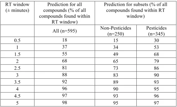
(10) correlation for the 92 reference standards was very good, with an R2 of 0.87. However, the current work is more wide-reaching, containing nearly 600 compounds of differing classes and physicochemical properties and is therefore expected to have a worse correlation. In order to improve this correlation, the 595 compounds were subdivided, not based on physicochemical parameters, solely on class, into two smaller subsets: pesticides and non-pesticides. The dataset initially contained pesticides, drugs of abuse, antibiotics, pharmaceuticals, veterinary drugs and mycotoxins. The vast majority of the compounds were pesticides (345 compounds), which made up one subgroup, while all the other compounds made up the other (250 compounds) (Figures S2 and S3). The “pesticides only” grouping did make for a scarcely better correlation (R2= 0.6947), while the “non-pesticides” had a slightly worse correlation (R2=0.6518), compared with the overall correlation (R2=0.6704). Although these correlations have rather large variability (especially for “non-pesticides”), it was thought to compare the predicted retention time (made from the equations, where “x” is the LogKow, in each of the figures) with the actual retention time for each compound. It was expected that there would be some deviation between the experimental and predicted retention times because it is difficult for the algorithm used by the LogKow predictor (ALOGPS 2.1) to cope with complex molecules, leading to some inaccurate LogKow values. Table 1 shows the differences between the predicted and actual retention times for the three cases. In spite of the variability of the data, the retention times of approximately 95% of the compounds were found within 4 minutes of their actual retention time. In the case of the. Page 10 of 27 .

(11) subsets, 79% of the pesticides can be found within 2 minutes of their actual retention time, which is 14% better than for non-pesticides. From these results, it was thought to use ± 2 minute window (± 11% of the chromatographic run) for use in real samples. The “pesticides only” predictor was selected for pesticides and “all compounds” for the other compounds, wherein approximately 80% and 70% of the compounds will be respectively found. This predictor was designed specifically for this precise chromatographic system, gradient and method. If applied to other separation systems, the correlation between LogKow and retention time for these particular compounds may differ widely. However, it is easy to adapt this retention time predictor to other systems using the methodology outlined in “Development of Retention Time Predictor”. Some groups have introduced a retention time index [6] to cope with this limitation. In order for a more complete predictor, training/validation sets comprising different compounds could be incorporated. Furthermore, the evaluation of different chromatographic conditions such as different columns and gradients could be carried out. Impact of experimental and predicted LogKow In an attempt to gain narrower retention time windows, a study was made on the impact of experimental versus predicted LogKow values. A study was made comparing the accuracy of predictive software, wherein ALOGPS 2.1 was shown to be quite accurate and only differed from the measured values by up to 0.5 Log units [15]. Software such as ALOGPS 2.1 is prone to systematic errors, especially for complex molecular structures, because correction factors for certain structural configurations might be missing [9]. To test the difference between experimental and predicted LogKow for the retention time predictors, “experimental” LogKow values were found for 280 of the. Page 11 of 27 .

(12) pesticides in the Pesticide Manual [20] and for 52 drugs of abuse, antibiotics, veterinary drugs and pharmaceuticals on DrugBank [21]. Figure 2 shows the difference between the experimental and predicted values for the 332 compounds at intervals of 0.1 Log units. As seen in the figure, fewer than 2% (corresponding to 5 of the 332 compounds) had the same experimental and predicted LogKow. Cumulatively, 77% of the compounds had an absolute difference within 1 Log unit; however 10% still had a difference greater than 2 Log units. These findings alone show that while predicted values give a good estimate, the fact that some compounds had a difference more than two Log values shows that experimentally derived values are preferable for any latter retention time predictions. The 36 compounds whose values of experimental and predicted LogKow differed by greater than 2 Log units were removed from the overall compound list to see the impact on the correlation coefficient. It was found that the R2 did not differ, with only a change from 0.6704 to 0.6737 following their removal (Figure S4). The difference between experimental and predicted LogKow values had such little impact on the correlation between LogKow and retention time, which gives credence to the use of predicted values. Furthermore, experimental values are not possible for all compounds and predicted values open up the possibility to work with new emerging contaminants and TPs, which is of particular relevance when investigating organic micropollutants in waters. Application of the retention time predictor to real water samples Fifteen influent wastewater and surface water samples were selected, representing different types of water sources, to test the retention time predictors. As stated previously, two predictors were used: one for pesticides only and one for nonPage 12 of 27 .

(13) pesticides. A set of 30 compounds were selected, based on their prevalence in environmental water samples [22–24] and their retention times were predicted using the aforementioned equations with the predicted LogKow of each of the compounds (Table S2). A retention time window of ± 2 minutes (from the predicted value) was given for each compound, and they were searched with a mass window of 20mDa. All peaks in the narrow window (nw)-XIC for each compound were counted manually (above intensity of 3000), while all peaks outside the prediction window were disregarded. All of the 30 compounds were detected in the water samples. Of these, 20 were found in the ± 2 minute retention time window (Figure 3). Remarkably, eight of the 20 compounds had only one peak inside the retention time window. In addition, the percentage of peaks outside the retention time window of ± 2 minutes (and therefore not pertaining to the compound of interest) was found to be 35%, meaning that over one third of the peaks in the XICs could be disregarded through retention time prediction. This retention time prediction shows a noticeable reduction in time spent processing data for potential positive samples.. Page 13 of 27 .

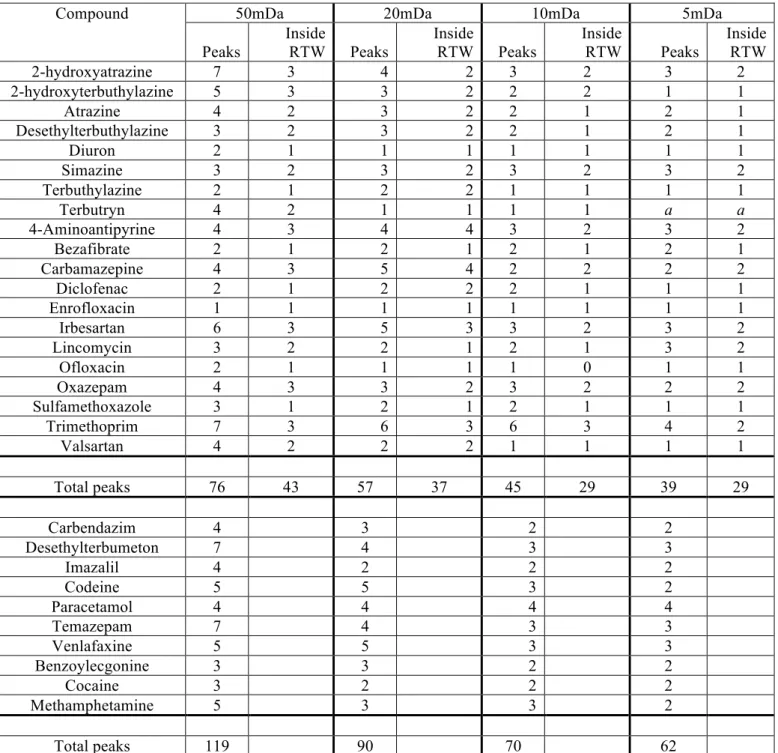
(14) Complementary use of mass chromatogram extraction window Using a mass window of 20mDa, four compounds only had one peak in the XIC (Figure 3). To complement the information and applicability of the retention time predictor, a comparison was made with three additional mass chromatogram extraction windows (50mDa, 10mDa and 5mDa). An extra window of 20mDa was used as a reference for these tests. The ten extra compounds, whose predicted retention time fell outside of the ± 2 minutes window, were also included in this test (see Table S2). The results of this comparison are shown in Table 2. As expected, the number of peaks observable in the XIC decreases as the extraction window decreases, from 119 (50 mDa) down to 62 peaks (5 mDa). However, it is of note that even at the 5mDa extraction window and within the retention time window, there were still unknown peaks not just pertaining to the compound of interest. In these situations, retention time prediction is very helpful in the reduction of false positive findings.. Page 14 of 27 .

(15) Figure 4 shows the influence of mass windows in XICs and the predicted retention time window for two compounds detected in surface water (benzoylecgonine, BE) and influent wastewater (trimethoprim). In the case of BE (major metabolite from cocaine), using a 50mDa XIC, several isobaric compounds are also seen; however, by decreasing the mass extraction window, all of these peaks disappear, leaving just the peak of BE at 4.53 minutes and a small spike at 6.5minutes. Although BE was able to be identified solely with a nw-XIC, the retention time fell just outside the predicted window (2.48 ± 2min). As stated above, the use of ± 2min retention time window led to a 70% success rate in the predictions for the “all compounds” group, where BE is included. Using a slightly wider window such as ± 2.5 min to get a success rate of 80%, similar to the pesticides group (see Table 1) would have led to BE being inside the prediction window. In any case, it seems that improvements are needed in the retention time prediction in order for it to be more useful in the identification process. In the case of the antibiotic trimethoprim, the peak is easily seen at 5mDa (3.66 minutes), however at a larger mass extraction window, two isobaric compounds are observed at a much higher intensity (2.5-3.0 minutes). With the retention time window (5.61 ± 2 min), these peaks, as well as the one at 7.6 minutes are removed, leaving just the two peaks at 3.66 and 4.6 minutes. The first one corresponded to trimethoprim, while the second was an unknown. This example shows the true utility of retention time prediction, especially in alliance with HRMS. While mass extraction windows can be narrowed to remove some interfering peaks, even at a 5mDa mass window, pseudoisobaric interferences remain. By incorporating retention time prediction, some of these false positive peaks can be removed.. Page 15 of 27 .

(16) Conclusions A critical evaluation has been made on the applicability of retention time prediction based on Log Kow to help in identification of suspect compounds in screening procedures. Two predictors were used; one based on pesticides only, and one for all other compounds (mainly licit and illicit drugs). Both were tested on 30 emerging contaminants commonly found in environmental and wastewater samples by retrospective analysis with QTOF-MS. In addition to help identify the compound of interest, the retention time predictors also allowed over one third of isobaric chromatographic peaks to be disregarded for further analysis as they were outside the retention time window, thereby enabling the reduction of tedious data processing. This is relevant when applying wide-scope screening for a large number of compounds (e.g. emerging contaminants and pesticides) or when investigating the presence transformation products, where many of the required reference standards are not available at the laboratory. In addition to the retention time prediction, the impact of extracted mass windows was investigated as a complementary tool for the screening. A smaller mass extraction window also removed unwanted peaks from the chromatogram. However, in some cases, even at a narrow mass extraction window of 5mDa, some isobaric peaks still appeared. The combination of this simple retention time predictor with extracted mass windows facilitated the removal of many false positives. In this work, 70-80% of compounds studied were able to be found in a ± 2 minute window, but a ±5 minute window was needed for ≥ 98% confidence. Our present research is focused on alternate and more sophisticated retention time predictors in order to improve the precision. This would allow the use of narrower time windows, thereby simplifying data processing due to fewer peaks needing to be investigated in the chromatograms. Page 16 of 27 .

(17) Acknowledgements The authors acknowledge the financial support provided by the Plan Nacional de I+D+I, Ministerio de Economía y Competitividad (Project ref CTQ2012-36189) and by Generalitat Valenciana (Group of Excellence Prometeo 2009/054, Prometeo II 2014/023; Collaborative Research on Environment and Food Safety ISIC/2012/016). Richard Bade acknowledges the European Union's Seventh Framework Programme for research, technological development and demonstration under Grant Agreement No. [Marie Curie-FP7-PEOPLE Grant #317205] for his Early Stage Researcher (ESR) contract.. Supplementary Information In this section, a table of the 595 compounds investigated, with their predicted LogKow values and empirical retention time is given (Table S1), as well as those compounds investigated in real samples, including their predicted and empirical retention time and precursor ion ([M+H]+) (Table S2). Furthermore, correlations of the Waters versus Inhouse compounds (Figure S1), pesticides only (n=345) with 95% confidence interval (Figure S2) and all other compounds (n=250) with 95% confidence interval (Figure S3) are included. Finally, a figure showing the impact on the removal of the compounds with an experimental Log Kow differing by more than 2 Log from the experimental value from the original LogKow-Retention time correlation is included (Figure S4) to provide supplementary information to the written text.. Page 17 of 27 .

(18) References [1]. S.D. Richardson, T.A. Ternes, Water analysis: emerging contaminants and current issues., Anal. Chem. 86 (2014) 2813–48. doi:10.1021/ac500508t.. [2]. B. Petrie, E.J. McAdam, M.D. Scrimshaw, J.N. Lester, E. Cartmell, M.E. J., Fate of drugs during wastewater treatment, TrAC Trends Anal. Chem. 49 (2013) 145– 159. doi:10.1016/j.trac.2013.05.007.. [3]. A. Agüera, M.J. Martínez Bueno, A.R. Fernández-Alba, New trends in the analytical determination of emerging contaminants and their transformation products in environmental waters., Environ. Sci. Pollut. Res. Int. 20 (2013) 3496–515. doi:10.1007/s11356-013-1586-0.. [4]. M.J. Gómez, M.M. Gómez-Ramos, O. Malato, M. Mezcua, A.R. FérnandezAlba, Rapid automated screening, identification and quantification of organic micro-contaminants and their main transformation products in wastewater and river waters using liquid chromatography-quadrupole-time-of-flight mass spectrometry with an accurate-mass , J. Chromatogr. A. 1217 (2010) 7038–54. doi:10.1016/j.chroma.2010.08.070.. [5]. F. Hernández, L. Bijlsma, J. V Sancho, R. Díaz, M. Ibáñez, Rapid wide-scope screening of drugs of abuse, prescription drugs with potential for abuse and their metabolites in influent and effluent urban wastewater by ultrahigh pressure liquid chromatography-quadrupole-time-of-flight-mass spectrometry., Anal. Chim. Acta. 684 (2011) 87–97. doi:10.1016/j.aca.2010.10.043.. [6]. A.C. Hogenboom, J.A. van Leerdam, P. de Voogt, Accurate mass screening and identification of emerging contaminants in environmental samples by liquid chromatography-hybrid linear ion trap Orbitrap mass spectrometry., J. Chromatogr. A. 1216 (2009) 510–9. doi:10.1016/j.chroma.2008.08.053.. [7]. M. Krauss, H. Singer, J. Hollender, LC-high resolution MS in environmental analysis: from target screening to the identification of unknowns, Anal. Bioanal. Chem. 397 (2010) 943–951. doi:10.1007/s00216-010-3608-9.. [8]. F. Hernández, M. Ibáñez, R. Bade, L. Bijlsma, J.V. Sancho, Investigation of pharmaceuticals and illicit drugs in waters by liquid chromatography-highresolution mass spectrometry, TrAC Trends Anal. Chem. 63(2014)140-157. doi:10.1016/j.trac.2014.08.003.. [9]. S. Kern, K. Fenner, H.P. Singer, R.P. Schwarzenbach, J. Hollender, Identification of transformation products of organic contaminants in natural waters by computer-aided prediction and high-resolution mass spectrometry, Environ. Sci. Technol. 43 (2009) 7039–7046. doi:10.1021/es901979h.. [10]. R. Díaz, M. Ibáñez, J. V Sancho, F. Hernández, Target and non-target screening strategies for organic contaminants, residues and illicit substances in food,. Page 18 of 27 .

(19) environmental and human biological samples by UHPLC-QTOF-MS, Anal. Methods. 4 (2012) 196–209. doi:10.1039/c1ay05385j. [11]. J. Nurmi, J. Pellinen, A.-L. Rantalainen, Critical evaluation of screening techniques for emerging environmental contaminants based on accurate mass measurements with time-of-flight mass spectrometry., J. Mass Spectrom. 47 (2012) 303–12. doi:10.1002/jms.2964.. [12]. T.R. Croley, K.D. White, J.H. Callahan, S.M. Musser, The chromatographic role in high resolution mass spectrometry for non-targeted analysis., J. Am. Soc. Mass Spectrom. 23 (2012) 1569–78. doi:10.1007/s13361-012-0392-0.. [13]. K. Héberger, Quantitative structure-(chromatographic) retention relationships., J. Chromatogr. A. 1158 (2007) 273–305. doi:10.1016/j.chroma.2007.03.108.. [14]. C. Giaginis, A. Tsantili-Kakoulidou, Quantitative Structure–Retention Relationships as Useful Tool to Characterize Chromatographic Systems and Their Potential to Simulate Biological Processes, Chromatographia. 76 (2012) 211–226. doi:10.1007/s10337-012-2374-6.. [15]. D. Livingstone, Theoretical Property Predictions, Curr. Top. Med. Chem. 3 (2003) 1171–1192. doi:10.2174/1568026033452078.. [16]. T.H. Miller, A. Musenga, D.A. Cowan, L.P. Barron, Prediction of chromatographic retention time in high-resolution anti-doping screening data using artificial neural networks., Anal. Chem. 85 (2013) 10330–7. doi:10.1021/ac4024878.. [17]. F. Hernández, M. Ibáñez, T. Portolés, M.I. Cervera, J. V Sancho, F.J. López, Advancing towards universal screening for organic pollutants in waters., J. Hazard. Mater. 282(2015) 86-95.doi:10.1016/j.jhazmat.2014.08.006.. [18]. M. Ibáñez, L. Bijlsma, A.L.N. van Nuijs, J. V Sancho, G. Haro, A. Covaci, et al., Quadrupole-time-of-flight mass spectrometry screening for synthetic cannabinoids in herbal blends., J. Mass Spectrom. 48 (2013) 685–94. doi:10.1002/jms.3217.. [19]. I. V Tetko, J. Gasteiger, R. Todeschini, A. Mauri, D. Livingstone, P. Ertl, et al., Virtual computational chemistry laboratory - design and description, J. Comput. Aided. Mol. Des. 19 (2005) 453–463. doi:10.1007/s10822-005-8694-y.. [20]. C.D.S. Tomlin, ed., The Pesticide Manual, Eleventh, British Crop Protection Council, Farnham, 1997.. [21]. D.S. Wishart, C. Knox, A.C. Guo, D. Cheng, S. Shrivastava, D. Tzur, et al., DrugBank: a knowledgebase for drugs, drug actions and drug targets, Nucleic Acids Res. 36 (2008) D901–6. doi:10.1093/nar/gkm958.. [22]. R. Díaz, M. Ibáñez, J. V Sancho, F. Hernández, Building an empirical mass spectra library for screening of organic pollutants by ultra-high-pressure liquid Page 19 of 27 . .

(20) chromatography/hybrid quadrupole time-of-flight mass spectrometry., Rapid Commun. Mass Spectrom. 25 (2011) 355–69. doi:10.1002/rcm.4860. [23]. E. Gracia-Lor, J. V Sancho, F. Hernandez, Multi-class determination of around 50 pharmaceuticals, including 26 antibiotics, in environmental and wastewater samples by ultra-high performance liquid chromatography-tandem mass spectrometry, J. Chromatogr. a. 1218 (2011) 2264–2275. doi:10.1016/j.chroma.2011.02.026.. [24]. N. 4/2011 Prescription data: IT del Sistema Nacional de Salud Volumen 35, Subgrupos ATC y Principios activos de mayor consumo en el Sistema Nacional de Salud en 2010, 2011.. Page 20 of 27 .

(21) Table 1: Comparisons between predicted and actual retention times RT window (± minutes). Prediction for all compounds (% of all compounds found within RT window) All (n=595). 0.5 1 1.5 2 2.5 3 3.5 4 4.5 5. 18 37 55 68 81 88 92 96 97 98. Prediction for subsets (% of all compounds found within RT window) Non-Pesticides (n=250) 15 34 49 65 73 83 89 90 93 95. Pesticides (n=345) 30 53 68 79 86 90 93 95 96 97. Page 21 of 27 .

(22) Table 2: Number of peaks found in the chromatograms (XICs) of 50mDa, 20mDa, 10mDa and 5mDa and inside the predicted retention time window. The lower compounds are those whose empirical retention times fall outside the ±2minute predicted retention time window Compound. 50mDa. 20mDa Inside RTW 3 3 2 2 1 2 1 2 3 1 3 1 1 3 2 1 3 1 3 2. 2-hydroxyatrazine 2-hydroxyterbuthylazine Atrazine Desethylterbuthylazine Diuron Simazine Terbuthylazine Terbutryn 4-Aminoantipyrine Bezafibrate Carbamazepine Diclofenac Enrofloxacin Irbesartan Lincomycin Ofloxacin Oxazepam Sulfamethoxazole Trimethoprim Valsartan. Peaks 7 5 4 3 2 3 2 4 4 2 4 2 1 6 3 2 4 3 7 4. Total peaks. 76. Carbendazim Desethylterbumeton Imazalil Codeine Paracetamol Temazepam Venlafaxine Benzoylecgonine Cocaine Methamphetamine. 4 7 4 5 4 7 5 3 3 5. 3 4 2 5 4 4 5 3 2 3. Total peaks. 119. 90. 43. Peaks 4 3 3 3 1 3 2 1 4 2 5 2 1 5 2 1 3 2 6 2 57. 10mDa Inside RTW 2 2 2 2 1 2 2 1 4 1 4 2 1 3 1 1 2 1 3 2. 37. Peaks 3 2 2 2 1 3 1 1 3 2 2 2 1 3 2 1 3 2 6 1 45 2 3 2 3 4 3 3 2 2 3 70. 5mDa Inside RTW 2 2 1 1 1 2 1 1 2 1 2 1 1 2 1 0 2 1 3 1. Peaks 3 1 2 2 1 3 1 a 3 2 2 1 1 3 3 1 2 1 4 1. 29. 39 2 3 2 2 4 3 3 2 2 2 62. a: not found in this mass extraction window. Page 22 of 27 . Inside RTW 2 1 1 1 1 2 1 a 2 1 2 1 1 2 2 1 2 1 2 1 29.

(23) Captions for Figures: Figure 1: Correlation between retention time and LogKow for all compounds, with 95% confidence interval Figure 2: Difference between experimental and predicted LogKow values and cumulative percentage of compounds within each differential interval. Figure 3: All 20 compounds found within the ± 2 minute retention time window and their associated peak data. The compounds on the left are all pesticides while those on the right are pharmaceuticals. The dark grey lines represent the average number of peaks found in the XIC of each compound and the light grey lines represent the average number of peaks inside the retention time window. Figure 4: TOP: XIC of Benzoylecgonine (m/z 290.139, 4.53 min) at 50mDa, 20mDa, 10mDa and 5mDa, with related predicted retention time window (2.48min ± 2 minutes) in surface water. BOTTOM: Trimethoprim (m/z 291.146, 3.64 min) and related retention time prediction window (Predicted retention time 5.61 min ± 2 minute window) at XICs of 50mDa, 20mDa, 10mDa and 5mD in influent wastewater. XICs at 10mDa, 20mDa and 50mDa all have been 5 times magnified (from 3 – 16 min) to highlight other peaks.. Page 23 of 27 .

(24) 25. y = 1.4957x + 4.7052 R² = 0.6704. Retention Time (min). 20 15 10 5 0 -‐4. -‐2. 0. 2. 4. 6. 8. 10. -‐5 -‐10. Log Kow. Figure 1. Page 24 of 27 .

(25) 100% 90%. Cumultive percentage of compounds. 80% 70% 60% 50% 40% 30%. 20% 10%. 0%. Difference between e xperimental and predicted values (Log units). Figure 2. Page 25 of 27 .

(26) 7 6. Number of peaks. 5 4. 20mDa (peaks in XIC) 20mDa (peaks inside RTW). 3 2 1. 0. Compound. Figure 3. Page 26 of 27 .

(27) . Figure 4 . Benzoylecgonine. %. ATTENAG_LC_008. 50 mDa. 4.53. 3 2.00 ATTENAG_LC_008. 4.00. 1: TOF MS ES+ 290.139 0.05Da 1.70e4. 6.00. 8.00. 10.00. 12.00. 14.00. 16.00. %. 1: TOF MS ES+ 290.139 0.02Da 1.68e4. 20 mDa. 4.53. 3 2.00 ATTENAG_LC_008. 4.00. 6.00. 8.00. 10.00. 12.00. 14.00. 16.00 1: TOF MS ES+ 290.139 0.01Da 6.03e3. 4.53. %. 10 mDa. 8 2.00 ATTENAG_LC_008. 4.00. 6.00. 8.00. 10.00. 12.00. 14.00. 16.00 1: TOF MS ES+ 290.139 0.00Da 5.99e3. 4.53. %. 5 mDa. 8. 2.00. 4.00. 2.48. 6.00. 8.00. 10.00. 12.00. 14.00. 16.00. Time. Trimethoprim EUDRUGS136. 1: TOF MS ES+ 291.146 0.05Da 9.79e5. x5. %. 50 mDa 3.66. 0. 2.00. 4.00. 6.00. 8.00. 10.00. 12.00. 14.00. 16.00. EUDRUGS136. 1: TOF MS ES+ 291.146 0.02Da 9.79e5. x5. %. 20 mDa 3.66. 0. 2.00. 4.00. 6.00. 8.00. 10.00. 12.00. 14.00. 16.00. EUDRUGS136. 1: TOF MS ES+ 291.146 0.01Da 9.78e5. x5. %. 10 mDa 3.66. 0. 2.00. 4.00. 6.00. 8.00. 10.00. 12.00. 14.00. 16.00. EUDRUGS136. 1: TOF MS ES+ 291.146 0.00Da 6.77e4. 5 mDa. %. 3.66. 1. 2.00. 4.00. 6.00. 5.61. 8.00. 10.00. 12.00. 14.00. 16.00. Time. . . Page 27 of 27 .

(28)