Measurement of the electroweak production of dijets in association with a Z boson and distributions sensitive to vector boson fusion in proton proton collisions at vs= 8 TeV using the ATLAS detector

Texto completo

(1)EUROPEAN ORGANISATION FOR NUCLEAR RESEARCH (CERN). CERN-PH-EP-2013-227. arXiv:1401.7610v2 [hep-ex] 15 Apr 2014. Submitted to: JHEP. Measurement of the electroweak production of dijets in association with a Z -boson and distributions sensitive to vector √ boson fusion in proton-proton collisions at s = 8 TeV using the ATLAS detector. The ATLAS Collaboration. Abstract Measurements of fiducial cross sections for the electroweak production of two jets in association with a Z -boson are presented. The measurements are performed using 20.3 fb−1 of proton-proton √ collision data collected at a centre-of-mass energy of s = 8 TeV by the ATLAS experiment at the Large Hadron Collider. The electroweak component is extracted by a fit to the dijet invariant mass distribution in a fiducial region chosen to enhance the electroweak contribution over the dominant background in which the jets are produced via the strong interaction. The electroweak cross sections measured in two fiducial regions are in good agreement with the Standard Model expectations and the background-only hypothesis is rejected with significance above the 5σ level. The electroweak process includes the vector boson fusion production of a Z -boson and the data are used to place limits on anomalous triple gauge boson couplings. In addition, measurements of cross sections and differential distributions for inclusive Z -boson-plus-dijet production are performed in five fiducial regions, each with different sensitivity to the electroweak contribution. The results are corrected for detector effects and compared to predictions from the Sherpa and Powheg event generators.. c 2014 CERN for the benefit of the ATLAS Collaboration. Reproduction of this article or parts of it is allowed as specified in the CC-BY-3.0 license..

(2) Prepared for submission to JHEP. Measurement of the electroweak production of dijets in association with a Z-boson and distributions sensitive to vector boson fusion in proton-proton √ collisions at s = 8 TeV using the ATLAS detector. ATLAS Collaboration. Abstract: Measurements of fiducial cross sections for the electroweak production of two jets in association with a Z-boson are presented. The measurements are performed using √ 20.3 fb−1 of proton-proton collision data collected at a centre-of-mass energy of s = 8 TeV by the ATLAS experiment at the Large Hadron Collider. The electroweak component is extracted by a fit to the dijet invariant mass distribution in a fiducial region chosen to enhance the electroweak contribution over the dominant background in which the jets are produced via the strong interaction. The electroweak cross sections measured in two fiducial regions are in good agreement with the Standard Model expectations and the background-only hypothesis is rejected with significance above the 5σ level. The electroweak process includes the vector boson fusion production of a Z-boson and the data are used to place limits on anomalous triple gauge boson couplings. In addition, measurements of cross sections and differential distributions for inclusive Z-boson-plus-dijet production are performed in five fiducial regions, each with different sensitivity to the electroweak contribution. The results are corrected for detector effects and compared to predictions from the Sherpa and Powheg event generators..

(3) Contents 1 Introduction. 1. 2 The ATLAS detector. 3. 3 Event reconstruction and selection. 4. 4 Theoretical predictions. 5. 5 Monte Carlo simulation. 6. 6 Fiducial cross-section measurements of inclusive Zjj production 6.1 Backgrounds 6.2 Systematic uncertainties 6.3 Comparison of data and simulation 6.4 Cross section determination. 7 9 9 11 11. 7 Differential distributions of inclusive Zjj production 7.1 Analysis methodology and unfolding to particle level 7.2 Systematic uncertainties 7.3 Unfolded differential distributions. 13 15 15 16. 8 Extraction of the electroweak Zjj fiducial cross section 8.1 Template construction and fit results 8.2 Validation of the control region constraint procedure 8.3 Systematic uncertainties on the fit procedure 8.4 Measurement of fiducial cross section 8.5 Estimate of signal significance 8.6 Limits on anomalous triple gauge couplings. 22 22 23 25 27 29 29. 9 Summary. 31. A Additional inclusive Zjj differential distributions. 32. 1. Introduction. The dominant production mechanism for a leptonically decaying Z/γ ∗ -boson1 in association with two jets (Zjj) at the Large Hadron Collider (LHC) is via the Drell–Yan process, with The contribution from γ ∗ production in association with two jets is substantially reduced in this analysis by an invariant mass cut on the Z/γ ∗ decay products. 1. –1–.

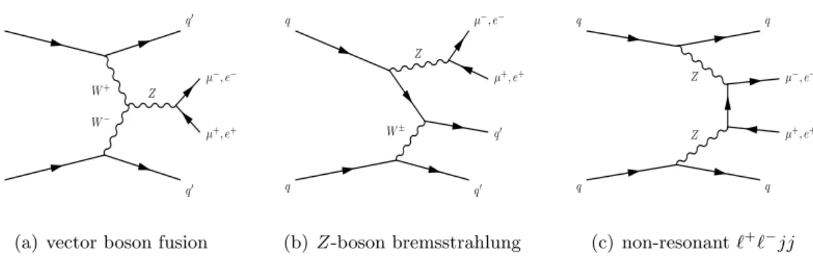
(4) q0. q. µ− , e−. q. q. q. Z W+. µ− , e−. W−. q. µ+ , e+. Z. µ− , e−. q0. Z. µ+ , e+. Z W±. µ+ , e+. q0. (a) vector boson fusion. q. q0. (b) Z-boson bremsstrahlung. q. q. (c) non-resonant `+ `− jj. Figure 1. Representative leading-order Feynman diagrams for electroweak Zjj production at the LHC: (a) vector boson fusion (b) Z-boson bremsstrahlung and (c) non-resonant `+ `− jj production.. the additional jets arising as a result of the strong interaction. Production of Zjj events via the t-channel exchange of an electroweak gauge boson is a purely electroweak process and is therefore much rarer. Electroweak Zjj production in the leptonic decay channel is defined to include all contributions to `+ `− jj production for which there is a t-channel exchange of an electroweak gauge boson [1, 2]. These contributions include Z-boson production via vector boson fusion (VBF), Z-boson bremsstrahlung and non-resonant production, as shown in figure 1. The VBF process is of particular interest because of the similarity to the VBF production of a Higgs boson and the sensitivity to anomalous W W Z triple gauge couplings.2 This paper presents two measurements of Zjj production using 20.3 fb−1 of protonproton collision data collected by the ATLAS experiment [3] at a centre-of-mass energy of √ s = 8 TeV: 1. Measurements of fiducial cross sections and differential distributions of inclusive Zjj production. These measurements are performed in five fiducial regions with different sensitivity to the electroweak component. Inclusive Zjj production is dominated by the strong production process, an example of which is shown in figure 2(a). The data therefore provide important constraints on the theoretical modelling of QCD-initiated processes that produce VBF-like topologies.3 2. Observation of electroweak Zjj production and measurements of the cross section in two fiducial regions. Limits are also placed on anomalous W W Z couplings. These measurements are performed using a combination of the Z → e+ e− and Z → µ+ µ− decay channels. Using electroweak Zjj production as a probe of colour-singlet exchange and as a validation of the vector boson fusion process has been discussed extensively in the literature [1, 4, 5]. A previous measurement by the CMS Collaboration showed evidence for 2. The VBF process cannot be isolated due to a large destructive interference with the electroweak Zboson bremsstrahlung process. The contribution to the electroweak cross section from non-resonant `+ `− jj production is less than 1% after applying the selection criteria used in this analysis. 3 Inclusive Zjj production contains a small (percent-level) contribution from diboson events (figure 2(b)).. –2–.

(5) q. q0. g. µ− , e− Z. µ− , e−. µ+ , e+. Z. q0 +. W±. +. µ ,e q. g. q. (a) strong Zjj production. q. q. (b) diboson-initiated. Figure 2. Examples of leading-order Feynman diagrams for (a) strong Zjj production and (b) diboson-initiated Zjj production.. √ electroweak Zjj production using proton-proton collisions at s = 7 TeV [6]. However, due to large experimental and theoretical uncertainties associated with the modelling of strong Zjj production, the background-only hypothesis could be rejected only at the 2.6σ level. The measurement presented in this paper constrains the modelling of strong Zjj production using a data-driven technique. This allows the background-only hypothesis to be rejected at greater than 5σ significance and leads to a more precise cross section measurement for electroweak Zjj production.. 2. The ATLAS detector. The ATLAS detector is described in detail in ref. [3]. Tracks and interaction vertices are reconstructed with the inner detector tracking system, which consists of a silicon pixel detector, a silicon microstrip detector and a transition radiation tracker, all immersed in a 2 T axial magnetic field, providing charged-particle tracking in the pseudorapidity range |η| < 2.5.4 The ATLAS calorimeter system provides fine-grained measurements of shower energy depositions over a wide range of η. An electromagnetic liquid-argon sampling calorimeter covers the region |η| < 3.2. It is divided into a barrel part (|η| < 1.475) and an endcap part (1.375 < |η| < 3.2). The hadronic barrel calorimeter (|η| < 1.7) consists of steel absorbers and active scintillator tiles. The hadronic endcap calorimeter (1.5 < |η| < 3.2) and forward electromagnetic and hadronic calorimeters (3.1 < |η| < 4.9) use liquid argon as the active medium. The muon spectrometer comprises separate trigger and high-precision tracking chambers measuring the deflection of muons in a magnetic field generated by superconducting air-core toroids. The precision chamber system covers the region |η| < 2.7 with three layers of monitored drift tube chambers, complemented by cathode strip chambers in the forward region, where the background is highest. The muon trigger system 4. ATLAS uses a right-handed coordinate system with its origin at the nominal interaction point (IP) in the centre of the detector and the z-axis along the beam pipe. The x-axis points from the IP to the centre of the LHC ring, and the y-axis points upward. Cylindrical coordinates (r, φ) are used in the transverse plane, φ being the azimuthal angle around the beam pipe. The pseudorapidity is defined in terms of the polar angle θ as η = − ln tan(θ/2). The rapidity is defined as y = 0.5 ln ((E + pz ) / (E − pz )), where E and pz refer to energy and longitudinal momentum, respectively.. –3–.

(6) covers the range |η| < 2.4 with resistive plate chambers in the barrel, and thin gap chambers in the endcap regions. A three-level trigger system is used to select interesting events [7]. The Level-1 trigger reduces the event rate to less than 75 kHz using hardware-based trigger algorithms acting on a subset of detector information. Two software-based trigger levels further reduce the event rate to about 400 Hz using the complete detector information.. 3. Event reconstruction and selection. √ The measurement is performed using proton-proton collision data recorded at s = 8 TeV. The data were collected between April and December 2012 and correspond to an integrated luminosity of 20.3 fb−1 . Events containing a Z-candidate in the µ+ µ− decay channel were retained for further analysis using a single-muon trigger, with muon transverse momentum, pT , greater than 24 GeV or 36 GeV (isolation criteria are applied at the lower threshold). Events containing a Z-candidate in the e+ e− decay channel were retained using a dielectron trigger with both electrons having pT > 12 GeV. In both decay channels, events are required to have a reconstructed collision vertex, defined by at least three associated inner detector tracks with pT > 400 MeV. The primary vertex for each event is then defined as the collision vertex with the highest sum of squared transverse momenta of associated inner detector tracks. Finally, the event is required to be in a data-taking period in which the detector was fully operational. Muon candidates are identified as tracks in the inner detector matched and combined with track segments in the muon spectrometer [8]. They are required to have pT > 25 GeV and |η| < 2.4. In order to suppress backgrounds, track quality requirements are imposed for muon identification, and impact parameter requirements ensure that the muon candidates originate from the primary vertex. The muon candidates are also required to be isolated: the scalar sum of the pT of tracks with ∆R < 0.2 around the muon track is required to be less than 10% of the pT of the muon. The radius parameter is defined as (∆R)2 = (∆η)2 + (∆φ)2 . Electron candidates are reconstructed from clusters of energy in the electromagnetic calorimeter matched to inner detector tracks. They are required to have pT > 25 GeV and |η| < 2.47, but excluding the transition regions between the barrel and endcap electromagnetic calorimeters, 1.37 < |η| < 1.52. The electron candidates must satisfy a set of ‘medium’ selection criteria [9] that have been reoptimised for the higher rate of protonproton collisions per beam crossing (pileup) observed in the 2012 data. Impact parameter requirements ensure the electron candidates originate from the primary vertex. Jets are reconstructed with the anti-kt jet algorithm [10] with a jet-radius parameter of 0.4. The input objects to the jet algorithm are three-dimensional topological clusters of energy in the calorimeter [11]. The resultant jet energies are initially corrected to account for soft energy arising from pileup [12]. The energy and direction of each jet is then corrected for calorimeter non-compensation, detector material and the transition between calorimeter regions, using a combination of MC-derived calibration constants and in situ data-driven calibration constants [13, 14]. Jets are required to have pT > 25 GeV and |y| < 4.4, where y is the rapidity. Additional data quality requirements are imposed to. –4–.

(7) minimise the effect of noisy calorimeter cells. To suppress jets from overlapping protonproton collisions, the jet vertex fraction (JVF) is used to identify jets from the primary interaction. Tracks are associated with jets using ghost-association [15], where tracks are assigned negligible momentum and clustered to the jet using the anti-kt algorithm. The JVF is subsequently defined as the scalar summed transverse momentum of associated tracks from the primary vertex divided by the summed transverse momentum of associated tracks from all vertices. Each jet with pT < 50 GeV and |η| < 2.4 is required to have JVF > 0.5. Finally, jets are required to be well separated from any of the selected leptons (jets within a cone of radius ∆R < 0.3 in η–φ space around any lepton are removed from the analysis).. 4. Theoretical predictions. Theoretical predictions for strong and electroweak Zjj production are obtained using the Powheg Box [16–18] and Sherpa v1.4.3 [19] event generators. The small contribution from diboson events is estimated using Sherpa. Sherpa is a matrix-element plus parton-shower generator that provides Z + n-parton predictions (n = 0, 1, 2...) at leading-order (LO) accuracy in perturbative QCD. The CKKW method is used to combine the various final-state topologies and match to the parton shower [20]. Electroweak Zjj production is accurate at LO for two and three partons in the final state. Strong Zjj production is accurate at LO for two, three and four partons in the final state, and the Z-boson plus zero and one parton configurations are also produced (at LO accuracy) to allow contributions from double parton scattering to be included. Diboson-initiated Zjj production (ZV ) is generated with up to three partons in addition to the partonically decaying boson. For all production channels, parton-shower, hadronisation and multiple parton interaction (MPI) algorithms create the fully hadronic final state. The Sherpa predictions are produced using the CT10 [21] parton distribution functions (PDFs) and the default generator tune for underlying event activity. The Powheg Box provides Zjj predictions at next-to-leading-order (NLO) accuracy in perturbative QCD for both electroweak and strong production [22–25]. The fully hadronic final state is produced by interfacing the Powheg Box to PYTHIA 6 [26], which provides parton showering, hadronisation and MPI. These particle level-predictions are referred to as Powheg in the remainder of this paper. The Powheg predictions are produced using the CT10 PDFs and the Perugia 2011 tune [27] for underlying event activity. The strong Zjj sample was generated with the MiNLO feature [28], which also produces Z plus zero and one jet events at LO accuracy and allows contributions to Zjj production from double parton scattering to be evaluated. Theoretical uncertainties are estimated for the strong and electroweak Zjj predictions from Sherpa and Powheg. Scale uncertainties on all theoretical predictions are estimated by varying the renormalisation and factorisation scales (separately) by a factor of 0.5 and 2.0. Additional modelling uncertainties in the Sherpa prediction arise from the choice of CKKW matching scale, the choice of parton-shower scheme, and the MPI-modelling.5 Similar 5. The uncertainty in the CKKW matching is determined by increasing the matching scale by a factor. –5–.

(8) modelling uncertainties in the Powheg prediction are estimated using the suite of Perugia 2011 tunes [27], with the largest effects coming from those tunes with increased/decreased parton-shower activity or increased MPI activity. The use of independent strong and electroweak Zjj samples relies on the fact that interference between the two processes is colour and kinematically suppressed, and therefore negligible. Interference between the strong and electroweak processes has been proven to be negligible for the production of the Higgs boson in association with two jets (Hjj) [32– 35]. Although no such studies have been performed for the electroweak production of a Zjj system, the interference effects arise from the same sources as Hjj production and should therefore be small. The assumption of negligible interference is checked for this measurement using a combined strong/electroweak Sherpa sample that is accurate to leading order for Zjj production. This combined sample includes electroweak and strong Zjj matrix elements at the amplitude level and thereby calculates the interference between them. The interference contribution is established by subtracting the strong-only and electroweak-only Zjj components. The impact of interference on inclusive Zjj cross sections and distributions is found to be negligible. The impact of interference on the extraction of the electroweak Zjj component is at the few-percent level and is discussed in more detail in section 8.. 5. Monte Carlo simulation. Event generator samples are passed through GEANT4 [36, 37] for a full simulation [38] of the ATLAS detector and reconstructed with the same analysis chain as used for the data. Pileup is simulated by overlaying inelastic proton-proton interactions produced with PYTHIA 8 [39], tune A2 [40] with the MSTW2008LO PDF set [41]. Strong and electroweak Zjj simulated events are produced using the Sherpa samples discussed in section 4. The samples are normalised to reproduce the NLO calculations for Zjj production obtained from Powheg; the NLO K-factors are 1.23 and 1.02 for the strong and electroweak samples, respectively. The contribution from ZV events is also produced using Sherpa. To cross-check aspects of the theoretical modelling of strong Zjj production at the detector level, a small simulated sample of Zjj events is produced using ALPGEN [42]. ALPGEN is a leading-order matrix-element generator that produces Z-boson events with up to five additional partons in the final state and is interfaced to HERWIG [43, 44] and JIMMY [45] to add the parton shower, hadronisation and MPI (AUET2 tune [46]). Background events stemming from tt̄ and single-top production are produced using MC@NLO v4.03 [47] interfaced to HERWIG and JIMMY (AUET2 tune). The generator modelling of tt̄ events is cross-checked with a simulated sample produced using the Powheg Box of two. Uncertainties associated with the parton shower are estimated by changing the recoil strategy for dipoles with initial-state emitter and final-state spectator, from the default [29] to that proposed in ref. [30]. The uncertainty due to a potential mismodelling of the underlying event is estimated by increasing the MPI activity uniformly by 10% [31], or changing the shape of the MPI spectrum such that more jets from double parton scattering are produced. The parameter variations for the latter are: SIGMA ND FACTOR=0.14 and SCALE MIN=4.0. –6–.

(9) interfaced to PYTHIA 6 (Perugia 2011 tune). The tt̄ samples are normalised to a next-tonext-to-leading-order (NNLO) calculation in QCD including resummation of next-to-nextto-leading-logarithmic (NNLL) soft gluon terms [48]. The backgrounds arising from W W and W +jets events are produced using Sherpa.. 6. Fiducial cross-section measurements of inclusive Zjj production. The cross section for inclusive Zjj production, σfid , is defined by Nobs − Nbkg σfid = R L dt · C. (6.1). where Nobs is the number of events observed in the data passing the reconstruction-level R selection criteria, Nbkg is the expected number of background events, L dt is the integrated luminosity and C is a correction factor accounting for differences in event yields at reconstruction and particle level due to detector inefficiencies and resolutions. The particle-level prediction is constructed using final-state particles with mean lifetime (cτ ) longer than 10 mm. Leptons are defined as objects constructed from the fourmomentum combination of an electron (or muon) and all nearby photons in a cone of radius ∆R = 0.1 in η–φ space centred on the lepton (so-called ‘dressed leptons’). Leptons are required to have pT > 25 GeV and |η| < 2.47. Jets are reconstructed using the anti-kt algorithm with a jet-radius parameter of 0.4. Jets are required to have pT > 25 GeV, |y| < 4.4 and ∆Rj,` ≥ 0.3, where ∆Rj,` is the distance in η–φ space between the jet and the selected leptons. The cross section for inclusive Zjj production is measured in five fiducial regions, each with different sensitivity to the electroweak component of Zjj production. A summary of the selection criteria for each fiducial region is given in table 1. The search region is chosen to optimise the expected significance when extracting the electroweak Zjj component, and is defined as: • A Z-boson candidate, defined as exactly two oppositely charged, same-flavour leptons with a dilepton invariant mass of 81 ≤ m`` < 101 GeV. • The transverse momentum of the dilepton pair must satisfy p`` T > 20 GeV. j1 • At least two jets that satisfy pT > 55 GeV, pjT2 > 45 GeV, where j1 and j2 label the highest and second highest transverse momentum jets in the event.. • The invariant mass of the two leading jets is required to satisfy mjj > 250 GeV. • No additional jets with pT > 25 GeV in the rapidity interval between the two leading jets. • The normalised transverse-momentum balance between the two leptons and the two highest transverse momentum jets, pbalance , is required to be less than 0.15. The T. –7–.

(10) Table 1. Summary of the selection criteria that define the fiducial regions. ‘Interval jets’ refer to the selection criteria applied to the jets that lie in the rapidity interval bounded by the dijet system. Object. baseline. high-mass. search. control. Leptons. |η ` | < 2.47, p`T > 25 GeV. Dilepton pair. 81 ≤ m`` ≤ 101 GeV p`` T > 20 GeV. —. —. |y j | < 4.4, ∆Rj,` ≥ 0.3. Jets. Dijet system. high-pT. pjT1 > 55 GeV. pjT1 > 85 GeV. pjT2 > 45 GeV. pjT2 > 75 GeV mjj > 250 GeV. mjj > 1 TeV. —. —. Interval jets. —. gap Njet =0. gap Njet ≥1. —. Zjj system. —. pbalance < 0.15 T. pbalance,3 < 0.15 T. —. pbalance is defined as T pbalance T. =. p~T`1 + p~T`2 + p~Tj1 + p~Tj2 p~T`1 + p~T`2 + p~Tj1 + p~Tj2. ,. (6.2). where p~Ti is the transverse momentum vector of object i, and `1 and `2 label the two leptons that define the Z-boson candidate. The tight cut on the dilepton invariant mass is chosen to suppress backgrounds from events that do not contain a Z-boson. The high-pT requirement on the two leading jets and the veto on additional jet activity preferentially suppress strong Zjj production with respect to electroweak Zjj production. The dijet invariant mass criterion removes a large fraction and p`` of diboson events. The pbalance T T requirements reduce the impact of those events containing jets that originate from pileup interactions or multiple parton interactions. Events with poorly measured jets are also removed by the pbalance requirement. T The control region criteria are chosen in order to suppress the electroweak Zjj contribution, allowing the theoretical modelling of strong Zjj production to be evaluated. The selection criteria are similar to the search region, with two modifications: (i) at least one additional jet with pT > 25 GeV must be present in the rapidity interval between the two leading jets. (ii) the transverse-momentum balancing variable is redefined to use the two leptons, the two highest transverse momentum jets, and the highest transverse momentum jet in the rapidity interval bounded by the two leading jets. This variable, pbalance,3 , is T balance defined in an analogous way to the pT variable in eq. (6.2), but incorporating the additional jet in the numerator and denominator. The remaining three fiducial regions are chosen with fewer selection criteria, in order to study inclusive Zjj production in simpler topologies. The baseline region is defined as. –8–.

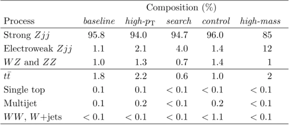
(11) containing a Z-boson candidate plus at least two jets with pjT1 > 55 GeV and pjT2 > 45 GeV. This is the most inclusive fiducial region examined and contains the events in all other fiducial regions. The high-mass region is chosen as the subset of these events that have mjj > 1 TeV. The high-pT region is defined as containing a Z-boson candidate plus at least two jets with pjT1 > 85 GeV and pjT2 > 75 GeV. The high-mass and high-pT regions are useful to probe the impact of the electroweak Zjj process, which produces a harder jet transverse momentum and harder dijet invariant mass than the strong Zjj process. The simulation-based correction factor (C) used to correct the measurement to the particle level is estimated using the Sherpa Zjj samples. The correction factor is found to lie between 0.80 and 0.92 in the muon channel, and between 0.64 and 0.71 in the electron channel, depending on the fiducial region. The difference between the channels arises primarily from the different efficiency in reconstructing and identifying electrons and muons in the detector. 6.1. Backgrounds. The contributions from the tt̄, W W , tW and W +jets background processes are obtained by applying the analysis chain to the dedicated simulated samples introduced in section 5. The multijet background contributes if two jets are misidentified as leptons or contain leptons from b- or c-hadron decays. A multijet sample is obtained from the data by reversing some of the electron identification criteria for the analysis in the electron channel, or reversing the muon isolation criteria for the analysis in the muon channel. The normalisation of the multijet sample in each fiducial region is then obtained by a two-component template fit to the dilepton invariant mass distributions, using the multijet template and a template formed from all other processes. Table 2 shows the composition by percentage of the predicted signal and background processes in each of the five fiducial regions. The event sample is dominated by processes producing a Z-boson in the final state. The dominant background to inclusive Zjj production is from tt̄ production. 6.2. Systematic uncertainties. The systematic uncertainties on the lepton reconstruction, identification, isolation and trigger efficiencies, as well as the lepton momentum scale and resolution, are defined in refs. [9, 49]. The total impact of the lepton-based systematic uncertainties on the crosssection measurement in each fiducial region is typically 3% in the electron channel and 2% in the muon channel. The uncertainty on the integrated luminosity is estimated to be 2.8%, using the methodology detailed in ref. [50] for beam-separation scans performed in November 2012. The jet energy scale (JES) and jet energy resolution (JER) uncertainties account for differences between the calorimeter response in simulation and data [13, 14, 51]. The JES uncertainty for 2012 data includes components for the soft-energy pileup corrections, the MC-based/data-driven calibration constants, the calibration of forward jets, and the. –9–.

(12) Table 2. Process composition (%) for each fiducial region for the combined muon and electron channels. The strong Zjj, electroweak Zjj, diboson, tt̄, W +jets and tW rates are estimated by running the analysis chain over MC samples fully simulated in the ATLAS detector. The multijet background is estimated using a data-driven technique.. Process Strong Zjj Electroweak Zjj W Z and ZZ tt̄ Single top Multijet W W , W +jets. baseline 95.8 1.1 1.0 1.8 0.1 0.1 < 0.1. Composition high-pT search 94.0 94.7 2.1 4.0 1.3 0.7 2.2 0.6 0.1 < 0.1 0.2 < 0.1 < 0.1 < 0.1. (%) control 96.0 1.4 1.4 1.0 < 0.1 0.2 < 1.1. high-mass 85 12 1 2 < 0.1 < 0.1 < 0.1. unknown jet flavour.6 The uncertainty due to JES is the dominant systematic uncertainty, ranging from 7.5% in the search region to 19% in the high-mass region. The uncertainty due to JER is much smaller, ranging from 0.1% in the high-pT region to 5% in the high-mass region. The JVF cut removes a fraction of the jets associated with the primary vertex in addition to the jets originating from pileup interactions. Any mismodelling of the JVF distribution therefore introduces a possible bias in the shape and normalisation of the distributions. A systematic uncertainty is determined after repeating the full analysis using modified JVF cuts that cover possible differences in efficiency between data and simulation. The JVF cuts are varied by ±0.03 and the uncertainty due to JVF modelling is found to be between 0.2% and 2.8% in the baseline and control regions, respectively. Hard jets originating from the additional (pileup) interactions are also reconstructed in the event and any mismodelling of pileup jets in the simulation is a source of systematic uncertainty. In the central calorimeter region, the JVF cut removes a large fraction of these jets. In the forward calorimeter regions (outside the inner detector acceptance), no track-based cut can be applied to remove these pileup jets. To estimate the impact of a possible mismodelling of the jets originating from pileup, the analysis is repeated using the simulated samples after removing pileup jets, defined as those reconstruction-level jets that are not matched (∆R ≤ 0.3) to a particle-level jet from the hard scattering process with pT > 10 GeV. The effect of pileup on each cross section measurement is then determined by comparing the reconstruction-level event yield obtained in simulation after applying jet matching to that obtained with no matching applied. Studies of the central jet transverse momentum in a pileup-enhanced sample (JVF < 0.1), and the transverse energy density in the forward region of the detector [52], indicate that the simulation could be mismodelling the number of pileup jets by up to 35%. The difference between the reconstruction-level 6. The jet flavour uncertainty refers to the different calorimeter response for quark-initiated and gluoninitiated jets.. – 10 –.

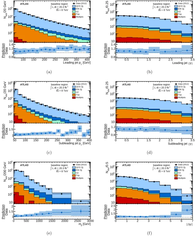
(13) event yields obtained with and without jet matching is therefore scaled by 0.35 and taken as a two-sided systematic uncertainty on the fiducial cross section. The impact on the final measurement is not large, ranging from less than 0.1% in the search region to 2.3% in the baseline region. In addition to the experimental uncertainties discussed above, systematic uncertainties on the correction factor, C, due to possible event generator mismodelling are evaluated. These generator modelling uncertainties are estimated by reweighting the events, at reconstruction level and particle level, such that the kinematic distributions in the simulation match those observed in the data. The reweighting is carried out for the two lepton transverse momenta and pseudorapidities, the two leading jet transverse momenta and pseudorapidities, and the variables used to define the fiducial regions. The correction factor is re-evaluated for each reweighting and the difference with respect to the nominal correction factor is taken as a theory modelling uncertainty. The uncertainty on the correction factor from theoretical modelling ranges from 1% in the baseline region to 6.6% in the high-mass region. The uncertainty due to background subtraction is found to be between 0.2% in the search region and 0.5% in the high-mass region. This accounts for the uncertainty in the normalisation of the inclusive tt̄ sample, generator modelling differences in tt̄ events predicted by MC@NLO and Powheg, and the uncertainty in the data-driven method used to determine the multijet background. The total systematic uncertainty on the inclusive Zjj cross-section measurement in each fiducial region is defined as the quadrature sum of all sources of experimental and theoretical uncertainty. 6.3. Comparison of data and simulation. Figure 3 shows data compared to MC simulation in the baseline region, as a function of the leading jet transverse momentum and rapidity, the subleading jet transverse momentum and rapidity, and the invariant mass and rapidity separation of the two leading jets. The uncertainty on the simulation due to the experimental systematic uncertainties is shown in the ratio as a hatched (blue) band. In general, the simulation gives an adequate description of the data, although there are indications of generator mismodelling at high jet transverse momentum and high dijet invariant mass. The contribution from tt̄ and multijet events remains small in each bin of the distributions. 6.4. Cross section determination. The cross sections are measured in the muon and electron decay channels separately. The cross-section measured in each fiducial region is found to be compatible between the two channels, with a maximum difference of 1.1σ after accounting for those uncertainties that are uncorrelated between channels. The results are then combined7 to obtain a weighted 7. The individual- and combined-channel cross sections are defined using dressed leptons as discussed in Section 6. Cross sections defined using ‘Born’ leptons (which originate directly from the Z-boson decay and before final state QED radiation) would differ by 2–3%.. – 11 –.

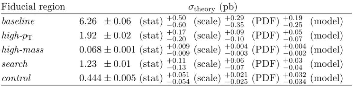
(14) baseline region. ∫ L dt = 20.3 fb. -1. s = 8 TeV. 4. 10. Nobs/0.25. Nobs/20 GeV. ATLAS. 105. Data (2012) QCD Zjj EW Zjj VZ Top Multijets. 106. -1. s = 8 TeV. 105. 10. 103. 102. 102. 10. 10 100. 150. 200. 250. 300. 350. 400. Prediction Data. 1.4 1.2 1 0.8. Leading jet p [GeV] T. 100. 150. 200. 250. 300 350 400 Leading jet pT [GeV]. 1.40 1.2 1 0.8 0. 0.5. 1. ATLAS. baseline region. ∫ L dt = 20.3 fb. -1. 5. 10. s = 8 TeV. 104. Data (2012) QCD Zjj EW Zjj VZ Top Multijets. 10. 3. 3.5. 0.5. 1. 1.5. 2. 2.5 3 3.5 Leading jet y. ATLAS. 106. baseline region. ∫ L dt = 20.3 fb. -1. s = 8 TeV. 105. Data (2012) QCD Zjj EW Zjj VZ Top Multijets. 103. 2. 10. 102. 10 50. 100. 150. 200. 250. 300. 350. 10. 400. Prediction Data. Prediction Data. 2.5. 104. 3. Subleading jet p [GeV]. 1.5. T. 1 50. 100. 150. 200. 0. 0.5. 1. 250 300 350 400 Subleading jet pT [GeV]. 0. ATLAS. baseline region. ∫ L dt = 20.3 fb. -1. 105. 2. 2.5. 3. 3.5. Subleading jet y. 0.5. 1. 1.5. 2. 2.5 3 3.5 Subleading jet y. (d). s = 8 TeV. 104. Nobs/0.5. 106. 1.5. 1.2 1 0.8. (c) Nobs/200 GeV. 2. (b) Nobs/0.25. Nobs/20 GeV. 106. 1.5. Leading jet y. (a). Data (2012) QCD Zjj EW Zjj VZ Top Multijets. 106. ATLAS. baseline region. ∫ L dt = 20.3 fb. -1. s = 8 TeV. 105. Data (2012) QCD Zjj EW Zjj VZ Top Multijets. 104. 103. 103. 2. 10. 102. 10 0. 2. 500. 1000. 1500. 2000. 3000. mjj [GeV]. 1.5 1 0. 2500. 500. 1000. 1500. 2000. 10. Prediction Data. Prediction Data. Data (2012) QCD Zjj EW Zjj VZ Top Multijets. baseline region. ∫ L dt = 20.3 fb. 104. 3. Prediction Data. ATLAS. 2500 3000 mjj [GeV]. (e). 2.50 2 1.5 1 0. 1. 2. 3. 4. 5. 6. 7. ∆y. 1. 2. 3. 4. 5. 6. ∆y. 7. (f). Figure 3. Comparison of data and simulation in the baseline region for (a,b) the leading jet transverse momentum and rapidity, (c,d) the subleading jet transverse momentum and rapidity, (e,f) the invariant mass and rapidity span of the dijet system. The simulated samples are normalised to the cross-section predictions discussed in section 5 and then stacked. The error bars reflect the statistical uncertainties of the data. The hatched band in the ratio reflects the total experimental systematic uncertainty on the simulation.. – 12 –.

(15) Table 3. Fiducial cross sections for inclusive Zjj production, measured in the Z → `+ `− decay channel.. Fiducial region baseline high-pT high-mass search control. 5.88 ± 0.01 1.82 ± 0.01 0.066 ± 0.001 1.10 ± 0.01 0.447 ± 0.004. (stat) (stat) (stat) (stat) (stat). σfid (pb) ±0.62 (syst) ±0.17 (syst) ±0.012 (syst) ±0.09 (syst) ±0.059 (syst). ±0.17 ±0.05 ±0.002 ±0.03 ±0.013. (lumi) (lumi) (lumi) (lumi) (lumi). Table 4. Theory predictions for inclusive Zjj production cross sections in the Z → `+ `− decay channel. The strong Zjj and electroweak Zjj events are produced using Powheg. A small contribution of ZV events, produced by Sherpa, is also included. The PDF uncertainty is estimated from the CT10 eigenvectors using the procedure described in ref. [21]. Scale and modelling uncertainties are each estimated from the envelope of Powheg sample variations discussed in section 4.. Fiducial region baseline high-pT high-mass search control. 6.26 ± 0.06 1.92 ± 0.02 0.068 ± 0.001 1.23 ± 0.01 0.444 ± 0.005. (stat) (stat) (stat) (stat) (stat). σtheory (pb) (scale) +0.29 −0.35 (scale) +0.09 −0.10 (scale) +0.004 −0.003 (scale) +0.06 −0.07 (scale) +0.021 −0.025. +0.50 −0.60 +0.17 −0.20 +0.009 −0.009 +0.11 −0.13 +0.051 −0.054. (PDF) (PDF) (PDF) (PDF) (PDF). +0.19 −0.25 +0.05 −0.07 +0.004 −0.002 +0.03 −0.04 +0.032 −0.034. (model) (model) (model) (model) (model). average, with each channel’s weight set to the inverse squared uncorrelated uncertainty. Table 3 presents the measured inclusive Zjj cross sections in the five fiducial regions together with their statistical and systematic uncertainties. Table 4 presents the Powheg prediction for strong and electroweak Zjj production, combined with the Sherpa prediction for the small contribution from diboson processes. Uncertainties on the theoretical predictions are broken down into statistical, scale, PDF and generator modelling uncertainties. Good agreement between data and theory is observed in all fiducial regions and a summary is shown in figure 4.. 7. Differential distributions of inclusive Zjj production. In this section, inclusive Zjj differential distributions are measured in the five fiducial regions presented in the previous section. The theoretical modelling of strong Zjj production is therefore confronted in regions with differing sensitivity to the electroweak Zjj component. The data are fully corrected for detector effects and are provided in HEPDATA [53] with full correlation information. The distributions sensitive to the kinematics of the two tagging jets are: •. 1 σ. dσ · dm : The normalised distribution of the dijet invariant mass of the two leading jj jets, mjj .. – 13 –.

(16) σZjj [pb]. 10. ∫. ATLAS L dt = 20.3 fb-1 s = 8 TeV. 1. Data 2012 10-1 σdata σtheory. 0.5. 1.1 1 0.9 0.8. Powheg (Zjj) + Sherpa (VZ) 1. baseline. 1.5. 2. 2.5. high p. T. 3. search. 3.5. 4. control. 4.5. 5. 5.5. high mass. Figure 4. Fiducial cross-section measurements for inclusive Zjj production in the Z → `+ `− decay channel, compared to the Powheg prediction for strong and electroweak Zjj production and the small contribution from ZV production predicted by Sherpa. The (black) circles represent the data and the associated error bar is the total uncertainty in the measurement. The (red) triangles represent the theoretical prediction, the associated error bar (or hatched band in the lower plot) is the total theoretical uncertainty on the prediction.. •. dσ · d|∆y| : The normalised distribution of the difference in rapidity between the two leading jets, |∆y|.. •. 1 dσ σ · d|∆φ(j,j)| :. 1 σ. The normalised distribution of the difference in azimuthal angle between the two leading jets, ∆φ(j, j).. The distributions sensitive to the difference in t-channel colour flow between electroweak and strong production of Zjj events include: •. 1 dσ gap : σ · dNjet. gap , with pT > 25 GeV The normalised distribution of the number of jets, Njet. in the rapidity interval bounded by the two highest-pT jets. •. 1 dσ : σ · dpbalance T. The normalised distribution of the pT -balancing distribution, pbalance (see T. eq. 6.2). • The fraction of events that contain no additional jets with pT > 25 GeV in the rapidity interval bounded by the two highest-pT jets (the jet veto efficiency) as a function of mjj and |∆y|. • The average number of jets with pT > 25 GeV in the rapidity interval bounded by gap the two highest-pT jets, hNjet i, as a function of mjj and |∆y|. • The fraction of events with pbalance < 0.15 (pbalance cut efficiency) as a function of T T mjj and |∆y|.. – 14 –.

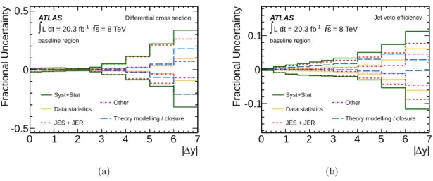
(17) 7.1. Analysis methodology and unfolding to particle level. The differential distributions are normalised to unity after subtracting the small background contributions from tt̄ and multijet events in each bin of the distributions. An iterative Bayesian unfolding procedure [54, 55] is then applied to the data to produce distributions at the particle level. This procedure uses a detector response matrix to reverse the bin migration caused by finite detector resolution. The response matrix is constructed from the strong and electroweak Zjj simulated samples for each distribution. Events that pass the reconstruction-level but not the particle-level selection criteria (or vice versa) are also corrected for as part of the unfolding procedure. The Bayesian unfolding procedure relies on knowledge of the underlying particle-level distribution. This ‘prior’ distribution is taken to be the particle-level prediction from Sherpa. After the first unfolding iteration, the input prior is replaced with the unfolded distribution from the data and the unfolding process is repeated. It is found that two iterations are sufficient to ensure convergence of the results. The statistical uncertainty on the data after unfolding is computed using pseudoexperiments. The statistical correlation between the numerator and the denominator in the jet veto distributions is retained by unfolding two-dimensional distributions constructed from the dijet observable (mjj , |∆y|) and information as to whether events passed or failed the efficiency criterion. The pbalance cut efficiency distribution is unfolded in a similar T gap way. Correlations in the hNjet i distributions are retained by unfolding a two-dimensional distribution constructed from the dijet observable and the number of jets in the rapidity interval between the two leading jets. Statistical correlations between bins from different unfolded distributions are estimated using a bootstrap method [56]. 7.2. Systematic uncertainties. The sources of experimental and theoretical uncertainty include all of those present in the measurement of the inclusive Zjj fiducial cross section (Sec. 6.2). The impact of leptonbased and luminosity systematic uncertainties on the measured distributions is negligible and the experimental systematic uncertainties therefore arise from JES, JER, JVF, as well as pileup jet modelling. The theoretical modelling uncertainties are again estimated by reweighting the simulation, such that the kinematic distributions of the variables used to define the fiducial regions match those observed in the data. An additional uncertainty associated with the closure of the Bayesian iterative procedure is estimated by reweighting the simulated events such that the reconstruction-level distribution being unfolded better matches the one observed in the data. The reweighting functions applied at the particle level are taken to be the ratio of the reconstruction-level distributions in data and simulation. For all sources of systematic uncertainty, the data are unfolded using a new response matrix constructed after shifting and smearing the MC events and objects. The shift in the unfolded spectrum is taken as the systematic uncertainty on the final result. The dominant uncertainties arise from the JES and JER, with small additional uncertainties from JVF, pileup modelling and theoretical modelling. The systematic uncertainties are presented in. – 15 –.

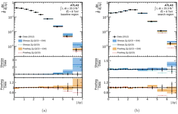
(18) ATLAS. ∫ L dt = 20.3 fb-1. Fractional Uncertainty. Fractional Uncertainty. 0.5. Differential cross section. s = 8 TeV. baseline region. 0 Syst+Stat Other Data statistics. -0.5 0. 2. 0.1. 3. 4. 5. 6. ∫ L dt = 20.3 fb-1. Jet veto efficiency. s = 8 TeV. baseline region. 0 Syst+Stat. -0.1. Theory modelling / closure. JES + JER. 1. ATLAS. Other Data statistics Theory modelling / closure. JES + JER. 7 |∆y|. 0. (a). 1. 2. 3. 4. 5. 6. 7 |∆y|. (b). dσ distribution and the jet veto Figure 5. Example systematic uncertainty breakdown for the σ1 · d|∆y| efficiency as a function of |∆y| in the baseline region. The effect of MC statistics, pileup modelling and JVF modelling are combined into one uncertainty labelled ‘other’.. dσ figure 5 for the σ1 · d|∆y| distribution and the jet veto efficiency as a function of |∆y|, in the baseline region. The total systematic uncertainty in each bin is defined as the quadrature sum of the individual sources of experimental and theoretical uncertainty. The unfolding procedure is cross-checked using the simulated ALPGEN sample in place of the Sherpa strong Zjj sample. The data are unfolded using the new response matrix formed from these simulated events. The data unfolded using the ALPGEN- and Sherpabased response matrices are found to agree, after accounting for the larger statistical uncertainty in the ALPGEN sample in addition to the theory modelling and closure uncertainties assigned to the nominal result.. 7.3. Unfolded differential distributions. The unfolded data are compared to particle-level predictions from Powheg and Sherpa in figures 6–10. The theoretical predictions are shown for combined electroweak and strong Zjj production and for strong Zjj production only. The theoretical uncertainty on the combined electroweak and strong Zjj prediction is estimated using the envelope of theory modelling uncertainties discussed in section 4. The contribution from diboson production is neglected for the theoretical predictions as the impact on the distributions is negligible. dσ dσ The unfolded σ1 · dm and σ1 · d|∆y| distributions are shown in figure 6 and 7, respecjj tively, for the baseline and search regions (corresponding distributions in the high-pT and control regions are provided in appendix A). Both of these distributions are sensitive to the difference between electroweak and strong production of Zjj events, especially at large mjj or |∆y|. In the electroweak process, the masses of the exchanged electroweak bosons lead to jets produced preferentially at large rapidities with sizeable transverse momentum. Furthermore, strong Zjj production typically involves the t-channel exchange of a spin-1/2 quark, which leads to steeper mjj and |∆y| spectra than the spin-1 exchange that is present. – 16 –.

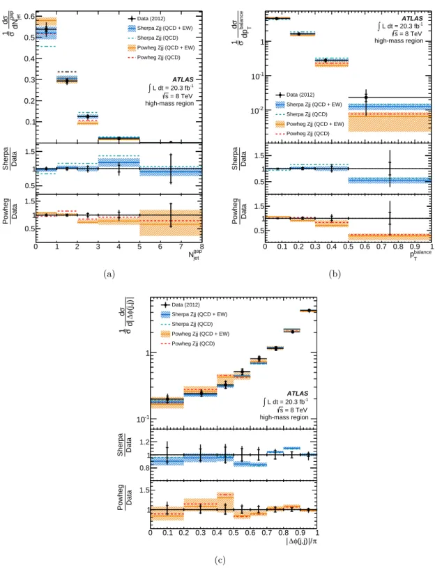
(19) jj. 1 dσ σ dm. jj. 1 dσ σ dm. Data (2012). 10-3. Sherpa Zjj (QCD + EW). Data (2012). 10-3. Sherpa Zjj (QCD + EW). Sherpa Zjj (QCD). Sherpa Zjj (QCD). Powheg Zjj (QCD + EW). 10-4. Powheg Zjj (QCD + EW). 10-4. Powheg Zjj (QCD). 10-5. 10-5 ATLAS. 10-6. 10-6. ∫ L dt = 20.3 fb. -1. s = 8 TeV baseline region. -1. 10-7 0. 500. 1000. 1500. 2000. 2500. 3000. 2 1.5. Sherpa Data. Sherpa Data. ATLAS. ∫ L dt = 20.3 fb s = 8 TeV search region. 10-7. 500. 1000. 1500. 2000. 2500. 1000. 1500. 2000. 2500. 3000. 500. 1000. 1500. 2000. 2500. 3000. 500. 1000. 1500. 2000. 1. 3000. Powheg Data. 0. 500. 1.2. 0.8. 1. Powheg Data. Powheg Zjj (QCD). 1.5 1. 1.2 1 0.8. 0. 500. 1000. 1500. 2000. 2500 3000 mjj [GeV]. (a). 2500 3000 mjj [GeV]. (b). dσ distribution in the (a) baseline and (b) search regions. The data Figure 6. Unfolded σ1 · dm jj are shown as filled (black) circles. The vertical error bars show the size of the total uncertainty on the measurement, with tick marks used to reflect the size of the statistical uncertainty only. Particle-level predictions from Sherpa and Powheg are shown for combined strong and electroweak Zjj production (labelled as QCD+EW) by hatched bands, denoting the model uncertainty, around the central prediction, which is shown as a solid line. The predictions from Sherpa and Powheg for strong Zjj production (labelled QCD) are shown as dashed lines.. in electroweak Zjj production. In the baseline region, the Powheg prediction is accurate to NLO in perturbative QCD and better describes the data at the highest values of mjj and |∆y| than Sherpa, which is accurate to LO. In particular, Sherpa predicts too large a fraction of events at large mjj and |∆y|, a feature also seen in previous measurements at the LHC and Tevatron [57, 58]. In the search region, the veto on additional jet activity means that both Sherpa and Powheg are accurate only to LO. Despite this, both predictions give a satisfactory description of the data if both strong and electroweak Zjj production are included. The contribution from electroweak Zjj production is evident at high mjj and high |∆y| in the search region for both event generators. dσ dσ The unfolded σ1 · dNdσgap , σ1 · dpbalance and σ1 · d|∆φ(j,j)| distributions are shown in the jet. T. high-mass region in figure 8. Quark/gluon radiation from the electroweak Zjj process is much less likely than in the strong Zjj process because there is no colour flow between the two jets. The contribution from electroweak Zjj production is clear in the low-multiplicity region of the σ1 · dNdσgap distribution for both Powheg and Sherpa, demonstrating the efjet. – 17 –.

(20) 1 dσ σ d ∆y. 1 dσ σ d ∆y. 1. ATLAS. ∫ L dt = 20.3 fb. -1. s = 8 TeV baseline region. 10-1. 1. -1. s = 8 TeV search region. 10-1. 10-2. 10-2 Data (2012). Data (2012). Sherpa Zjj (QCD + EW). Sherpa Zjj (QCD + EW). Sherpa Zjj (QCD). 10-3. Sherpa Zjj (QCD). 10-3. Powheg Zjj (QCD + EW). Powheg Zjj (QCD + EW). 0. 3. 1. 2. Powheg Zjj (QCD). 3. 4. 5. 6. 7. 2. Sherpa Data. Powheg Zjj (QCD). Sherpa Data. ATLAS. ∫ L dt = 20.3 fb. 0. 1. 2. 3. 4. 5. 6. 7. 1. 2. 3. 4. 5. 6. 7. 1. 2. 3. 4. 5. 6. 1.5 1. 1 1. 2. 3. 4. 5. 6. 7. 0. Powheg Data. Powheg Data. 0. 1.2 1 0.8 0. 1.2 1 0.8. 1. 2. 3. 4. 5. 6. ∆y. 7. 0. (a). ∆y. 7. (b). dσ Figure 7. Unfolded σ1 · d|∆y| distribution in the (a) baseline and (b) search regions. The data and theoretical predictions are presented in the same way as in figure 6.. fectiveness of the jet veto at separating the strong and electroweak components of Zjj dσ production. Both Powheg and Sherpa adequately describe the data for the σ1 · dpbalance and T. dσ · d|∆φ(j,j)| distributions; the latter distribution has little sensitivity to the electroweak 8 process. gap i distributions as a function Figure 9 shows the unfolded jet veto efficiency and hNjet of mjj and |∆y| in the baseline region (corresponding distributions in the high-pT region are provided in appendix A). These variables probe the theoretical description of wideangle quark and gluon radiation in strong Zjj events as a function of the energy scale of the dijet system. For the electroweak process, quark and gluon radiation into the rapidity interval is suppressed and little jet activity is expected. This is evident at medium-tohigh values of mjj , for which the strong Zjj prediction has more jet activity than the combined strong and electroweak Zjj prediction. In general, both theoretical predictions give a good description of the data (for combined strong and electroweak Zjj production), although Sherpa gives a slightly better description than Powheg when compared across both the mjj and |∆y| distributions. Sherpa and Powheg have previously provided a good description of the jet activity in the rapidity interval bounded by a dijet system in purely 1 σ. 8. Although the azimuthal angle between the jets is not sensitive to the differences between strong and electroweak Zjj production, it is of interest in Higgs-plus-two-jet studies, as the vector boson fusion and gluon fusion production channels have very different azimuthal structure [59–61].. – 18 –.

(21) 0.5. -1. T. dσ. ATLAS. ∫ L dt = 20.3 fb. dp. Sherpa Zjj (QCD + EW). balance. Data (2012). Sherpa Zjj (QCD). s = 8 TeV high-mass region. 1. 1 σ. jet. 1 dσ σ dNgap. 0.6. Powheg Zjj (QCD + EW) Powheg Zjj (QCD). 0.4 0.3. 10-1. ATLAS -1 ∫ L dt = 20.3 fb s = 8 TeV high-mass region. 0.2. Data (2012) Sherpa Zjj (QCD + EW). 10-2. Sherpa Zjj (QCD). 0.1. Powheg Zjj (QCD + EW). 1.5. 1. 2. 3. 4. 5. 6. 7. 8. 0. Sherpa Data. Sherpa Data. Powheg Zjj (QCD). 0. 1. 0.2. 0.3. 0.4. 0.5. 0.6. 0.7. 0.8. 0.9. 1. 0.1. 0.2. 0.3. 0.4. 0.5. 0.6. 0.7. 0.8. 0.9. 1. 1.5 1 0.5. 0.5 1. 2. 3. 4. 5. 6. 7. 8. 0. Powheg Data. 0. Powheg Data. 0.1. 1.5 1. 1.5 1. 0.5 0. 0.5 1. 2. 3. 4. 5. 6. 7. 8. 0. gap. Njet. 0.1 0.2 0.3 0.4 0.5 0.6 0.7 0.8 0.9 1 pbalance T. (b) dσ 1 σ d ∆φ(j,j). (a). Data (2012) Sherpa Zjj (QCD + EW) Sherpa Zjj (QCD) Powheg Zjj (QCD + EW) Powheg Zjj (QCD). 1. ATLAS. ∫ L dt = 20.3 fb. -1. s = 8 TeV high-mass region. Sherpa Data. 10-1 0. 0.1. 0.2. 0.3. 0.4. 0.5. 0.6. 0.7. 0.8. 0.9. 1. 0.1. 0.2. 0.3. 0.4. 0.5. 0.6. 0.7. 0.8. 0.9. 1. 1.2 1 0.8. Powheg Data. 0. 1.5 1 0. 0.1 0.2 0.3 0.4 0.5 0.6 0.7 0.8 0.9 1 ∆φ(j,j) / π. (c) dσ dσ Figure 8. Unfolded (a) σ1 · dNdσgap , (b) σ1 · dpbalance distributions in the high-mass and (c) σ1 · d|∆φ(j,j)| jet T region. The data and theoretical predictions are presented in the same way as in figure 6.. – 19 –.

(22) Jet veto efficiency. Jet veto efficiency. 1. Data (2012) Sherpa Zjj (QCD + EW). 0.9. Sherpa Zjj (QCD). 0.8. Powheg Zjj (QCD + EW) Powheg Zjj (QCD). 0.7 0.6. -1. s = 8 TeV baseline region. 0.9 0.8. Data (2012). 0.6. 0.4 0.3. ATLAS -1 ∫ L dt = 20.3 fb s = 8 TeV baseline region. Sherpa Zjj (QCD + EW) Sherpa Zjj (QCD). 0.5. Powheg Zjj (QCD + EW) Powheg Zjj (QCD). 0.4. 0. 500. 1000. 1500. 2000. 2500. 3000. 1.2 1. Sherpa Data. 0.2 Sherpa Data. ∫ L dt = 20.3 fb. 0.7. 0.5. 1.20. 1. 2. 3. 4. 5. 6. 7. 1. 2. 3. 4. 5. 6. 7. 1. 2. 3. 4. 5. 6. 1 0.8. 0.8. 0.6 500. 1000. 1500. 2000. 2500. 3000. 0. Powheg Data. 0. Powheg Data. ATLAS. 1. 1.5 1. 1.2 1 0.8. 0. 500. 1000. 1500. 2000. 2500 3000 mjj [GeV]. 0. gap. Data (2012). 1.2. Sherpa Zjj (QCD + EW). 1. Powheg Zjj (QCD + EW). Sherpa Zjj (QCD) Powheg Zjj (QCD + EW) Powheg Zjj (QCD). 0.5 0.4 0.3. 0.4. ATLAS -1 ∫ L dt = 20.3 fb s = 8 TeV baseline region. 0. 500. 1000. 1500. 2000. 2500. ATLAS. 0.2. ∫ L dt = 20.3 fb. -1. s = 8 TeV baseline region. 0.1 3000. 1.2 1. Sherpa Data. 0.2 Sherpa Data. Sherpa Zjj (QCD + EW). 0.6. 0.6. 0.8. 0. 1. 2. 3. 4. 5. 6. 7. 1. 2. 3. 4. 5. 6. 7. 1. 2. 3. 4. 5. 6. 1.2 1 0.8. 500. 1000. 1500. 2000. 2500. 3000. 0. Powheg Data. 0. Powheg Data. Data (2012). 0.8 0.7. Sherpa Zjj (QCD). Powheg Zjj (QCD). 0.8. 7. (b) ⟨Njet ⟩. gap. ⟨Njet ⟩. (a). ∆y. 1. 1 0.8. 0.5 0. 1.2. 500. 1000. 1500. 2000. 2500 3000 mjj [GeV]. (c). 0. ∆y. 7. (d). gap i versus (c) Figure 9. Unfolded jet veto efficiency versus (a) mjj and (b) |∆y|, and unfolded hNjet mjj and (d) |∆y|. All distributions are measured in the baseline region. The data and theoretical predictions are presented in the same way as in figure 6.. – 20 –.

(23) 0.95. ATLAS. Data (2012). ∫ L dt = 20.3 fb. -1. Sherpa Zjj (QCD + EW). s = 8 TeV baseline region. Sherpa Zjj (QCD). 0.9. pbalance < 0.15 cut efficiency. Powheg Zjj (QCD + EW) Powheg Zjj (QCD). 0.85 0.8 0.75. 1. ATLAS. Data (2012). ∫ L dt = 20.3 fb. -1. Sherpa Zjj (QCD + EW). 0.9. s = 8 TeV baseline region. Sherpa Zjj (QCD) Powheg Zjj (QCD + EW) Powheg Zjj (QCD). 0.8 0.7. T. T. pbalance < 0.15 cut efficiency. 1. 0.7. 0.6. 0.65 0.5 1000. 1500. 2000. 2500. 3000. 1 0.8 1.2. 0. Powheg Data. 500. 500. 1000. 1500. 2000. 2500. 3000. 500. 1000. 1500. 2000. 1.20. 2500 3000 mjj [GeV]. (a). 1. 2. 3. 4. 5. 6. 7. 1. 2. 3. 4. 5. 6. 7. 1. 2. 3. 4. 5. 6. 1 0.8 1.2. 0. 1 0.8 0. Sherpa Data. 1.20. Powheg Data. Sherpa Data. 0.6. 1 0.8 0. ∆y. 7. (b). Figure 10. Unfolded pbalance cut efficiency versus (a) mjj and (b) |∆y| in the baseline region. The T data and theoretical predictions are presented in the same way as in figure 6.. dijet topologies [31, 62]. The unfolded pbalance cut efficiency as a function of mjj and |∆y| in the baseline region T is shown in figure 10 (the corresponding distribution in the high-pT region is provided in appendix A). Again, with less quark/gluon radiation from the electroweak process, it is expected that the two jets are better balanced against the Z-boson for the electroweak Zjj process than for the strong Zjj process. This is apparent at high mjj and high |∆y|, where the strong Zjj prediction falls below the data. For this distribution, Powheg describes the data poorly at low values of mjj or |∆y|, whereas Sherpa gives a good description of the data over the full range of the distributions. In general, neither Sherpa nor Powheg is able to fully reproduce the data for all distributions in all fiducial regions. Powheg gives a better description of the data than Sherpa for the mjj and |∆y| distributions, with Sherpa predicting too large a cross section at the highest values of mjj or |∆y|. However, Sherpa gives a better description for variables sensitive to the additional jet activity in the event, with Powheg predicting too little jet activity in the rapidity interval bounded by the dijet system. The unfolded data can be used to constrain the modelling of Zjj production in the extreme phase-space regions probed in this measurement. The unfolded data are provided in HEPDATA with statistical and systematic uncertainties. Furthermore, the correlation between bins of different distributions is provided, allowing the quantitative comparison of all distributions simultaneously.. – 21 –.

(24) 8. Extraction of the electroweak Zjj fiducial cross section. The electroweak Zjj component is extracted by fitting the dijet invariant mass reconstructed in the search region. Templates are formed for the signal and background processes and a fit to the dijet invariant mass distribution in the data is performed, allowing the normalisation of each template to float. The fit is performed using a log-likelihood maximisation [63] and the number of signal and background events is extracted. The number of signal events is then converted into a fiducial cross section, using a correction factor to convert from the reconstruction-level event selection to the particle-level event selection. 8.1. Template construction and fit results. The signal template is obtained from the Sherpa electroweak Zjj sample. The background template is constructed from the Sherpa strong Zjj sample plus the small contribution from the diboson and tt̄ samples (the other background sources are found to have negligible impact on the results). The background template is then constrained using the following data-driven technique. The dijet invariant mass distributions are constructed for data and MC simulation in the control region and a reweighting function is defined by fitting the ratio of the data to MC simulation with a second-order polynomial. This reweighting function is then applied directly to the background template in the search region. The data are therefore used to constrain the generator modelling of the background mjj shape, and the MC simulation is used only to extrapolate this constraint between the control and search regions. This procedure has the advantage of minimising both the experimental and theoretical systematic uncertainties on the background template. Figure 11(a) shows the dijet invariant mass distribution in the control region for the data and the MC simulation for the electron and muon channels combined. The reweighting function is shown in the lower panel. The use of the control region to constrain the background template is validated in section 8.2 and corresponding systematic uncertainties are presented in section 8.3. Figure 11(b) shows the dijet invariant mass distribution in the search region for the electron and muon channels combined. The signal and background templates are normalised to the values obtained from the fit. The background template is presented after the datadriven reweighting using the second-order polynomial in figure 11 (a). The unconstrained background template is also compared to the data in the lowest panel, demonstrating that the background-only prediction always falls below the data at high-mjj . Table 5 summarises the fit results, giving the number of signal (NEW ) and background (Nbkg ) events expected by the MC simulation and the number obtained from the fit, together with the statistical uncertainties from the data (first uncertainty) and MC templates (second uncertainty). The results are shown for electrons and muons separately and also with both channels combined, where the latter result is obtained by combining the two channels for the data and for the MC templates before fitting. For the purpose of measuring the fiducial cross section, the yields from the fits to electrons and muons are used. For the purpose of determining systematic uncertainties on NEW , which are correlated between the two channels, the fractional shift in the number of events obtained from the fit combining both channels is used.. – 22 –.

(25) Nobs / 250 GeV. Nobs / 250 GeV. 104. ATLAS. ∫ L dt = 20.3 fb. -1. s = 8 TeV control region. 103. ATLAS. ∫ L dt = 20.3 fb. 104. -1. s = 8 TeV search region. 103 102. 102. 10 Data (2012). 10. Data (2012). Background. 1000. 1500. 2000. 2500. 3000. p + p mjj + p m2jj 0. 1. 3500. 2. p + p mjj 0. 1. 1 0.5 500. BKG BKG + EW Data Data. Data MC. 500. 1.5. Background. 1. Background + EW Zjj. 1.5. 500. 1000. 1500. 2000. 2500. 3000. 500. 1000. 1500. 2000. 2500. 3000. 3500. 1 0.5 1 0.5 0. 1000 1500 2000 2500 3000 3500 mjj [GeV]. Background + EW Zjj. 3500 mjj [GeV]. constrained unconstrained. 500. 1000 1500 2000 2500 3000 3500 mjj [GeV]. (a). (b). Figure 11. (a) The dijet invariant mass distribution in the control region. The simulation has been normalised to match the number of events observed in the data. The lower panel shows the reweighting function used to constrain the shape of the background template. (b) The dijet invariant mass distribution in the search region. The signal and (constrained) background templates are scaled to match the number of events obtained in the fit. The lowest panel shows the ratio of constrained and unconstrained background templates to the data.. Table 5. The number of strong (Nbkg ) and electroweak (NEW ) Zjj events as predicted by the MC simulation and obtained from a fit to the data. The number of events in data is also given. The first and second uncertainties on the fitted yields are due to statistical uncertainties in data and simulation, respectively. The first and second uncertainties in the MC prediction are the experimental and theoretical systematic uncertainties, respectively.. Data MC predicted Nbkg MC predicted NEW Fitted Nbkg Fitted NEW. 8.2. Electron 14248 13700 ± 1200 +1400 −1700 602 ± 27 ± 18 13351 ± 144 ± 29 897 ± 92 ± 27. Muon 17938 18600 ± 1500 +1900 −2300 731 ± 29 ± 22 17201 ± 161 ± 31 737 ± 98 ± 28. Electron+muon 32186 32600 ± 2600 +3400 −4000 1333 ± 50 ± 40 30530 ± 216 ± 40 1657 ± 134 ± 40. Validation of the control region constraint procedure. The data-driven background constraint derived in the control region is an important component of the analysis as it improves the modelling of the background mjj spectrum and constrains the impact of experimental and theoretical uncertainties. Several cross-checks are performed to validate the method.. – 23 –.

(26) The choice of polynomial used to describe the reweighting function is investigated by using a first-order polynomial instead of a second-order polynomial. The lower panel of figure 11(a) shows that both choices of polynomial give very similar reweighting functions at low mjj and differ only at the highest values of mjj . The change in NEW is less than 2% if the first-order polynomial is used to reweight the background template in place of the second-order polynomial. The choice of event generator is examined by reweighting the simulated dijet invariant mass distribution for strong Zjj production using the ratio of the Powheg and Sherpa particle-level predictions. This reweighting is carried out in the search and control regions separately. Powheg has been shown to give a much better description of the data for the dijet invariant mass in figure 6 for all fiducial regions. The reweighting to Powheg improves the description of the data in the control region. The data-driven reweighting function then becomes much flatter and repeating the full analysis procedure with the new templates produces a result consistent at 0.8% with the analysis based on the Sherpa samples alone. The choice of control region is studied by splitting it into six subregions that probe the additional jet activity in the rapidity interval between the two leading jets. The control and search regions are distinguished by this additional jet activity and these subregions allow the impact of any mismodelling in the simulation to be explored. Two subregions are defined by the transverse momentum of the leading jet in the rapidity interval (25 < pT ≤ 38 GeV and pT > 38 GeV), two subregions are defined by the rapidity of the jet (|y| ≤ 0.8 and |y| > 0.8), and two subregions are defined by the number of jets in the rapidity interval (Njet = 1 and Njet ≥ 2). In addition to these six regions, an MPI-suppressed subregion jj is defined by the requirements |∆φ(j, j)/π| < 0.9 and pjj T > 20 GeV, where pT is the transverse momentum of the dijet system. This region allows the impact of MPI on the control region constraint to be examined. Figure 12(a) shows the background reweighting functions obtained from these subregions, compared to the default function obtained from the default control region. The extraction of the electroweak signal is cross-checked using each of these constraints. The values of NEW are consistent, with a maximum 5% spread between subregions. This spread is likely to be statistical in origin, as the values of NEW obtained from reweighting functions derived in orthogonal subregions are found to agree to better than 1σ when considering only the statistical uncertainty associated with the reweighting functions. Although the spread of reweighting functions in figure 12(a) is large at high mjj , the background modelling in this region has only a small impact on the extracted number of electroweak Zjj events. The background modelling shape has most impact at values of mjj around 1–1.5 TeV, for which the spread of reweighting functions is just a few percent. The orthogonal subregions are also used to test the agreement between data and the corrected simulation directly. The reweighting function derived in the pT > 38 GeV subregion is used to correct the simulation in the 25 < pT ≤ 38 GeV subregion, as shown in figure 12(b). The corrected simulation gives a better description of the data than the uncorrected simulation. Similar tests are performed for the subregions split by jet rapidity or jet multiplicity. In all cases, the corrected simulation gives a better description of data. – 24 –.

(27) 0.9 0.8 0.7 0.6. Data MC. Data MC. ATLAS control region s = 8 TeV. 1. control region with 25 < p ≤ 38 GeV T s = 8 TeV. 1.1. default y ≤ 0.8 y > 0.8 Njet = 1 Njet ≥ 2 p > 38 GeV T 25 < p ≤ 38 GeV. 1 0.9 0.8 0.7. T. 0.5. ATLAS. 1.2. ∆φ(j,j)/π < 0.9, jj p > 20 GeV. 0.6. T. 500 1000 1500 2000 2500 3000 3500. uncorrected MC: χ2/Ndf = 10.9/5 corrected MC: χ2/Ndf = 3.3/5. 500. 1000. mjj [GeV] (a). 1500 2000 mjj [GeV]. (b). Figure 12. (a) Background reweighting functions obtained for different choices of control region. (b) The agreement between data and simulation in the 25 < pT ≤ 38 GeV subregion both before and after applying a background reweighting function derived in the pT > 38 GeV subregion.. than the uncorrected simulation. 8.3. Systematic uncertainties on the fit procedure. Systematic uncertainties on NEW arise from the background template reweighting function, the jet-based experimental systematic uncertainties, and the theoretical modelling uncertainties on the Zjj samples. The uncertainty due to the lepton-based systematic uncertainties is negligible. A summary of the systematic uncertainties discussed in this section is presented in table 6. The systematic uncertainty due to the limited number of events in the control region is obtained using pseudo-experiments, and is found to be 8.9% and 11.2% in the electron and muon channels, respectively. The remaining experimental systematic uncertainties affect the extracted value of NEW by changing the shape of the signal template and/or the shape of the background template. The experimental systematic uncertainties that change the template shape are due to JES, JER, JVF, as well as pileup jet modelling, as discussed in section 6.2. The effect on the number of fitted events due to each source of uncertainty is evaluated simultaneously for signal and background templates in order to account for correlations. Systematic variations in the signal template are evaluated by taking the ratio of the template formed with a systematic shift to the nominal template, fitting that ratio with a second-order polynomial, applying that polynomial as a reweighting function to the signal template, and repeating the fit for the number of electroweak events. The use of the polynomial to estimate the systematic shift reduces the impact of statistical fluctuations. – 25 –.

(28) at large mjj . For the systematic variations in the background template, the data provide a constraint in the control region, meaning that only the effect of each systematic variation on the extrapolation between the control and search regions needs to be evaluated. A double ratio is formed from the systematic-shifted to nominal ratios in the search and control regions and fitted with a first-order polynomial function. If the gradient of the fitted function is statistically significant, defined as the parameter value being greater than 1.64 times the parameter uncertainty, then this component is considered as a significant source of systematic uncertainty. This significance requirement is chosen to remove 90% of statistical fluctuations and avoid double counting statistical uncertainties in the simulated samples.9 For each significant source of systematic uncertainty, the first-order polynomial is applied as an additional reweighting to the background template in the search region and the fit is repeated. The dominant systematic uncertainty on the extracted value of NEW from experimental sources is from the JES (5.6%). This uncertainty comes almost entirely from the uncertainty on the signal template shape, because the shape of the background template is constrained using the control region. The uncertainty due to the JVF is modest (1.1%), whereas the uncertainty from JER and pileup modelling is effectively negligible (0.4% and 0.3%, respectively). Additional uncertainties on the extraction of the electroweak component arise from the theoretical modelling in the MC generators. Again, these affect the signal template as well as the extrapolation between the control and search region for the background template. The uncertainties due to theoretical modelling are split into two components: PDF modelling and generator modelling. Uncertainties due to PDF modelling are obtained as follows. The nominal value of NEW is obtained using the CT10 PDF set. The full analysis is then repeated using simulated samples created using (i) the CT10 uncertainties and (ii) the central values and uncertainties of two other PDF sets, MSTW2008nlo [41] and NNPDF2.3 [64]. Each PDF variation is applied to the signal and background simultaneously. For each PDF set, the uncertainty on NEW is then calculated using the recommended procedure from each collaboration [65, 66], with the CT10 results scaled to reflect 68% probability. The αs uncertainty is found to be negligible. The overall uncertainty due to PDF modelling is found to be +1.5 −3.9 % from the envelope of uncertainties obtained from each PDF set. The generator modelling uncertainties are determined using the dedicated Sherpa sample variations discussed in section 4, by varying the factorisation and renormalisation scale, varying the activity from multiple parton interactions (MPI), and changing the partonshower scheme or CKKW matching parameters. To evaluate the generator modelling uncertainty, the analysis is repeated for each sample variation independently to obtain a shift in NEW . The standard deviation in the shifted values for each sample variation is obtained using a pseudo-experiment approach. The effect of the signal modelling uncertainty on 9. The choice of significance requirement was investigated by changing the requirement to 1.0 or 2.0. The resultant systematic uncertainties were unchanged from the nominal choice of 1.64.. – 26 –.