Tecnol´ogico de Costa Rica Escuela de Ingenier´ıa Electr´onica
Static Hand Pose Recognition
on Depth Images
(Reconocimiento de pose est´atica de manos en im´agenes de profundidad)
Documento de tesis sometido a consideraci´on para optar por el grado acad´emico de Maestr´ıa en Electr´onica con ´Enfasis en Procesamiento Digital de Se˜nales
Declaro que el presente documento de tesis ha sido realizado enteramente por mi per-sona, utilizando y aplicando literatura referente al tema e introduciendo conocimientos y resultados experimentales propios.
Resumen
Con el aumento del uso de nuevas tecnolog´ıas en actividades diarias, la demanda de sistemas de interacci´on humano-m´aquina (HCI por sus siglas en Ingl´es) ha incrementado. Sistemas de reconocimiento de pose de manos han sido ampliamente explorados para dicha tarea debido a su operaci´on intuitiva para usuarios inexpertos. Sin embargo, el reconocimiento de pose de manos basados en visi´on es un problema extremadamente desafiante debido a la din´amica de la mano, la cual posee un gran n´umero de grados de libertad que la hacen dif´ıcil de estimar y conlleva a problemas adicionales como la auto oclusi´on. Con el desarrollo se sistemas de visi´on confiables y asequibles para el usuario com´un como el Microsoft Kinect©, las im´agenes de profundidad se han convertido en una herramienta ´util para el reconocimiento de partes del cuerpo y por tanto, para el reconocimiento de manos.
Abstract
With the increasing usage of new technologies in common daily activities, the demand of efficient human-computer interaction (HCI) systems increases. Hand pose recognition systems have been widely explored for such task due to its intuitive operation for non experienced users. However, vision-based hand pose recognition is a extremely challenging problem due to the dynamics of the hand, which poses a large amount of degrees of freedom that makes it difficult to estimate and carries out additional problems such as self occlusion. With the development of reliable and consumer affordable vision systems such as the Microsoft Kinect©, depth imaging has become a useful tool on body parts recognition and thus, for hand recognition.
Acknowledgements
First of all, I thank my family and friends for all the support given in those years, I would never have made it without them.
Additionally, I would like to thank my supervisor Dr. Pablo Alvarado Moya and the Dr. Alexander Singh Alvarado for their guidance and advice during the development of my thesis, providing me a valuable experience and knowledge.
Contents
List of Figures iii
List of Tables v
Glossary vii
1 Introduction 1
1.1 Objective and Thesis Organization . . . 3
2 Related works 5 3 Foundations 7 3.1 Decision Trees . . . 7
3.1.1 Training Process . . . 8
3.1.2 Prediction Process . . . 11
3.2 Random Decision Forests . . . 12
3.2.1 Randomness Model . . . 12
3.3 Support Vector Machines . . . 13
3.4 Hu Moments in Image Processing . . . 15
3.4.1 Geometric Moments . . . 16
3.4.2 Moment Invariants . . . 16
4 Recognition of Static Hand Poses from a Top View 19 4.1 System Architecture . . . 19
4.2 The Data Set . . . 20
4.3 Phase 1: Pixel Segmentation using RDF . . . 22
4.4 Visual Features for Hand Pose Classification . . . 23
4.5 Phase 2: Gesture Classification . . . 27
ii Contents
5.4.2 Classification Using SVM . . . 39
5.4.3 Classification of Ideal Predicted Blobs using RDF . . . 40
6 Conclusions 43
6.1 Future Work . . . 44
List of Figures
1.1 General diagram of global concept . . . 2
3.1 Graphical description of a binary decision tree . . . 8
3.2 Decision tree training algorithms . . . 10
3.3 Prediction process for a decision tree . . . 11
3.4 Graphical description of random decision forest . . . 12
3.5 Features space separation using hyperplanes. . . 14
3.6 Feature space mapping using kernels . . . 15
4.1 General diagram of the system developed . . . 20
4.2 Generated depth image without shadow (left) and with shadows (right) . . 21
4.3 Example of Curfil’s feature calculation in a depth image . . . 22
4.4 Features extraction process for hand pose classification . . . 24
4.5 Location of the hand’s wrist . . . 25
4.6 Hand ROI for histogram calculation . . . 25
4.7 Hand ROI quadrants for histogram calculation . . . 26
4.8 Hand regions extraction and Hu moments calculation from rotated image . 27 5.1 Classification error vs RDF configuration for different features . . . 36
5.2 Classification error vs RDF size for different depth values using the entire features set . . . 37
5.3 Misclassification of pointing class pixels . . . 38
List of Tables
3.1 Common kernel functions used for SVM . . . 15
3.2 Geometric properties of a two-dimensional digital image based on its moments 17 4.1 Hand classes, depth image and ground truth masks . . . 21
4.2 Data sets (50% images with shadow) . . . 22
4.3 Features for hand pose classification . . . 27
5.1 Data sets used for experimental results (50% images with shadow) . . . 29
5.2 Hand pose samples at different location/rotation values . . . 30
5.3 RDF configuration for hand segmentation . . . 31
5.4 Confusion matrix for RDF A trained with depth images without noise . . . 31
5.5 Confusion matrix for RDF B trained with noisy depth images . . . 32
5.6 Confusion matrix for RDF C trained with mixed depth images . . . 32
5.7 Class accuracy omitting background class prediction statistics . . . 32
5.8 Experimental hand segmentation results for RDF A, B and C . . . 33
5.9 Relative wrist point distance measurements for RDF predicted images . . . 34
5.10 Relative wrist point distance for xand y coordinates . . . 34
5.11 Experimental visual features used for hand pose classification . . . 35
5.12 RDF configuration used for hand pose classification . . . 35
5.13 Best classification error and average per-class accuracy using all features . 36 5.14 Best classification error and average per-class accuracy using all features . 37 5.15 Confusion matrix for hand classification using the complete set of features 38 5.16 Features importance percentage for an RDF trained with all the features sets . . . 39
5.17 Parameters range used for SVM grid analysis . . . 40
5.18 Classification error and average per-class accuracy for SVM classifier (γ = 0.0001,C = 5.275) . . . 40
Glossary
Abreviaciones
IR Infrared
RDF Random Decision Forest
RNO Randomized Node Optimization ROI Region Of Interest
Chapter 1
Introduction
Human-computer interaction (HCI) has taken a key role in the modern society due to the latest technology advances that have increased the usage of computer based systems in common daily activities. Within the whole range of applications using vision based systems, hand controlled systems are widely extended due to their easy use and intuitive nature. Hands provide a dexterous functionality in communication and manipulation that makes them a perfect tool for any interactive application[11] compared with other approaches such as face or voice control. The usage of hand recognition-based systems covers a wide range of applications such as virtual reality and simulation [3, 29], mobile devices [30], sign language recognition [29], musical gestures recognition [7], among others. Despite hands are acknowledged as an effective interaction tool, they carry out a set of challenges in regards with their detection using computer vision systems[11]:
• Dimensionality: With approximately 27 degrees of freedom, the hand pose is highly difficult to estimate compared with simpler recognition systems such as body pose recognition [8, 21, 11].
• Self-occlusion: Due to the amount of degrees of freedom, the hand suffers of self-occlusion, i.e., on a variety of positions and points of view from the camera, some sections of the hand are occluded by others avoiding its direct estimation with vision computer systems[26, 17, 8].
• Noise: The range sensors available nowadays present a relatively high level of noise in the depth information (e.g. Gaussian noise with standard deviation of 1cm at 1m distance for PrimeSense sensors)[26,11, 8].
2
processing frame rates over 20fps. However most of the available proposals for hand recognition require a powerful system to run on such timing conditions, making them infeasible for the market.
With the introduction of the depth sensor at an accessible cost for the common user, most of those challenges discussed above have been resolved or treated on a simpler way providing a new field of research for hand recognition. Despite all the improvements provided by depth sensors for image processing application and more specific for hand recognition, usually they are used together with color sensors for complementary image processing[23, 10, 22]. Additionally, some common assumptions such as distance to the camera and location constrains are usually taken when dealing with depth images, to simplify the whole processing pipeline.
This thesis is part of a global concept to approach the estimation of hand joints of multiple hands in a single scene from a top view, using depth images only. The general proposal is divided in three major processing stages as depicted in figure1.1: the first stage aims to the detection of one or more hands on a depth image scene and provide the approximated location. The second stage uses the input information to segment the hand region and predict the intended hand posture. Finally, the third stage processes the depth blob and the posture information to estimate the joints of the hand within the depth image.
Hand detector Hand pose
estimator
Figure 1.1: General diagram of global concept
1 Introduction 3
1.1
Objective and Thesis Organization
Chapter 2
Related works
There is a plethora of research work aiming the analysis and recognition of hands using computer vision, due to the range of possible applications. With the development of depth sensors at low cost such as the Microsoft Kinect© or the Intel Creative Gesture Camera©, the field of research involving depth images for hand analysis has gained momentum. Several approaches have been proposed for hand gesture and pose recognition using depth images. Keskin et al. [17] present a pose estimation algorithm for commonly used hand postures. They use a random decision forest (RDF) for per pixel classification and the mean shift algorithm is used to estimate the position of the joints. Their results are demostrated with a American Sign Language (ASL) digits classifier using the joints esti-mation.
Kuznetsova et al. [18] use a multi-layered random forest (MLRF) and ensemble of shape (ESF) to classify 24 hand postures from ASL depth images. They extract the point cloud from the 2D images and use the MLRF to cluster it in the first layer. The second layer in the MLRF is used to assign the corresponding hand pose to the data set. In [9] a different approach is taken to estimate the hand shape from depth data. In this case a sequence of widths is extracted from the hand contour and axis of elongation in order to be compared with a pre-defined synthetic data set using several similarity measurements. The hand segmentation is done under the premise that the hand is the closest object to the camera, so a simple threshold function can be applied.
6
vector machine (SVM) is then used to classify the features.
Pugeault and Bowden [22] use random decision trees to classify 24 hand postures of the ASL captured with a Microsoft Kinect. They use OpenNI[1] to localize the hand position and establish a region of interest around it on the depth and color images. Then a Garbor filter is used to get a feature vector from depth and intensity data that is going to be used to train an RDF for classification.
Chapter 3
Foundations
This master’s thesis focuses on the recognition of static hand poses from a top view using depth images. Some specific topics such as random decision forests, support vector ma-chines among others are used in the implementation. This chapter aims to the description of those methods.
Section 3.1 provides a brief introduction to decision trees for classification, including the training and prediction processes. In section 3.2 the concept of decision tree is extended to random decision forest. Section3.3 provides an insight in the theory of support vector machines. Finally section 3.4explains the basics of geometric moments to present the Hu moments.
3.1
Decision Trees
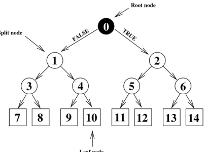
As stated in [6], a decision tree can be defined as a special type of graph composed of nodes and edges as shown in figure 3.1for a binary tree. A tree starts from an upper root node and splits up downwards into several internal nodes until it ends up at the terminal nodes commonly called leaf nodes in the N th-level (where N is the tree’s depth). The simplest arrangement of nodes for a decision tree is called binary decision tree, where each node splits up in at most two children: left and right.
8 3.1 Decision Trees
Figure 3.1: Graphical description of a binary decision tree (depth = 4)
3.1.1
Training Process
As described previously, a decision tree starts its training process from the root node splitting up the incoming data set into two groups: left and right. This splitting process continues on each node until it reaches a terminal node. This way each leaf node li allocates a distribution function p(c|li(x)) for each class label c and the input data x. Different estimators can be implemented in order to interpret such distribution function, being the most common method to select the class with the highest probability.
The training process can be summarized as an iterative process, executed for each node in the tree as follows[28, 6]:
1. Select a set ofdata points. Each data point corresponds to an specific sample within the entire data set.
2. Compute a set of features v = {x1, x2, ..., xd} on each data point with v ∈ Rd. Ideally the dimensiond for each feature space can be infinite, however in practice a subset of the whole features space is used instead.
3. Once the features are calculated for the data points, a test functionτ(θ) withθ ∈Θ is used to split the set in left and right samples. θ represents the parameter set of the test function belonging to the entire parameter space Θ.
3 Foundations 9
5. Once the best split function has been selected the resulting left and right data sets are passed to the next layer nodes and the process is applied recursively.
6. Each leaf node stores a probability distribution p(c|v), based on the total of data points that reach the node and the corresponding label. This way each leaf provides a measure of the probability for a data point with a features set v to belong to an specific class c.
7. The training finishes until a stop criterion is met.
From the algorithm described above four key concepts have direct impact in the training process:
a) Feature function: the features used commonly for decision trees have the pecu-liarity of being weak compared with the complexity of the classification performed by the entire structure. They are completely dependent of the application and the data set used. For example Shotton et al. in [25] use the difference between two pixels in the neighborhood of the current point as the feature function for body parts detection in depth images. Waldvogel in [28] uses the difference of two regions in the neighborhood of the pixel as the feature function in order to create a per-pixel classifier using depth and color images.
b) Split function: The test functionτ works on the computed features based on a set of split parameters θ and takes a decision about which branch the sample belongs to, such that
τ(v, θt)→ {true, f alse} ∀θt ∈Θ (3.1) Commonly the test function is a simple threshold value that can be set on advance or can be randomly selected.
c) Objective function: Also called score function, it evaluates each test function and helps to determinate the best split criteria for the current node. One of the most frequently used objective functions is the information gain. For a binary decision tree the information gain is defined as[6]
I =H(S)− X S
i
10 3.1 Decision Trees
In short, the analysis of the objective function I can be seen as a maximization problem at each note jth for the data points in the node Sj and the specific split parameters set θ as follows
θj = argmax θ
I(Sk, θ) (3.3)
d) Stop criteria: Growing full trees can be possible but impractical since it leads to over-fitted trees with low or zero generalization capability. Is for this reason that having an adequate stop criterion is a critical aspect of the training process. Diverse stopping criteria can be applied to a decision tree, being the most common the depth or number of levels of the tree. Alternatively other criteria can be used such as establishing a threshold for the objective function, determining the level of entropy in the leaf nodes. On the other hand the number of samples per node can be limited as a stop criterion avoiding the tree to overfit.
An interesting property of decision trees is that the chronological order of calculating node splits does not influence the decision tree structure[28], this gives rise to variants in the training process in regards with the order of nodes generation. Two main algorithms are widely used: depth-first training and breadth-first training. The former grows each child recursively until the stop criterion hold before it moves to the next adjacent node. In the case of breadth-first method all nodes on the same level are trained before moving to the next level. Figure3.2 depicts both training methods, where numbers represent the order on which the algorithm processes the nodes and the dashed nodes represent future nodes to be processed.
Figure 3.2: Decision tree training algorithms. (a) Depth-first method. (b) Breadth-first method.
When the training process has finished, three data sets are obtained that describe the tree entirely:
1. The best split functions for each node. 2. The tree structure.
3 Foundations 11
The major drawback of decision trees is its training time, which can be considerable when dealing with big data sets. This disadvantage has encouraged the research of acceleration methods for the training process such as in [28].
3.1.2
Prediction Process
The prediction process starts in the same way as the training, splitting up the data set from the root node downwards to reach the leaf nodes.
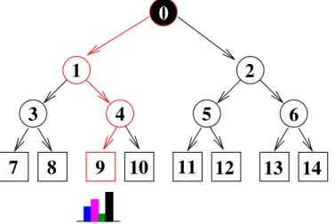
From the training process each node was associated with an specific test function that minimize the entropy. When predicting new unseen data, the tree computes the corre-sponding features and splits it according to the training information. Since this process is only executed on the nodes involved on each split calculation the algorithm does not have to got through all the nodes within the tree. Figure 3.3 exemplifies the prediction path (in red) for a data point within a decision tree, it only requires the calculation of three nodes to reach a terminal node (represented with squares).
4
7
8
9
2
6
5
0
1
3
10
11
12
13
14
Figure 3.3: Prediction process for a decision tree. The processing path of a data point is marked in red.
12 3.2 Random Decision Forests
3.2
Random Decision Forests
A Random Decision Forest (RDF) is an ensemble learning method constructed by a set of random decision trees as shown in figure3.4 for an RDF comprised of 3 decision trees with 4 levels each one.
p1 p3
Tree 1 Tree 2 Tree 3
p2
Figure 3.4: Graphical description of random decision forest (T = 3 anddepth= 4). The 3 prediction paths are marked in red, blue and green producing 3 corresponding probability distributions.
In an RDF each tree is trained independently as described in section3.1.1. The prediction is computed for each data point in all trees producing a set of T different probability distributions (where T is the forest size) as depicted in figure3.4.
Several prediction models are used to determinate the final output of the forest, being the most common the calculation of the average probability distribution as follows[6]
p(c|v) = 1
The training and testing process in an RDF is achieved independently for each tree within the forest. This characteristic provides high parallelism leading to very efficient software implementations.
3.2.1
Randomness Model
Randomization is done in the training phase with the goal to improve the generalization capability of the classifier. There are two commonly used methods to inject randomness[6]:
1. Bagging
2. Randomized node optimization
3 Foundations 13
chosen from the original data set for each treet. Having a different random training set for each tree leads to the generation of different training parameter avoiding specialization. Randomized node optimization (RNO) consists of training each node with a different random subset of split parameters Θt taken from the whole parameter space Θ, varying the set of possible tests performed on the features for each node. The more data points in Θ are contained in Θt (such that Θt ≈ Θ), the more similar become the trees in the ensemble and the lower randomness is achieved, decreasing the generalization of the forest. Randomness methods are not mutual exclusive which means that they can be implemented together in regards to the application requirements.
Summarizing, a set of six key parameters have a direct effect over the RDF training process as well as its prediction capabilities[6]:
1. The tree depthD
2. The size of the forestT
3. The objective function I for the training process 4. The feature function
5. The test functionτ
6. The randomness methods injected
3.3
Support Vector Machines
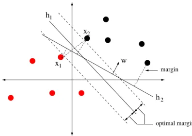
Support Vector Machines (SVM), also known as support vector networks, are super-vised learning methods for pattern recognition commonly used for binary classification applications[2, 16]. SVMs start from the basic concept of hyperplane separation. Con-sider a feature set S ={x1, . . . ,xi} with xi ∈ Rd (where d is the dimension of each data point); it may be possible to find an hyperplane w·x+b= 0 that splits the data points in regards to their class labels.
Figure 3.5 shows an example of plane separation for two different hyperplanes h1, h2. In
14 3.3 Support Vector Machines
Figure 3.5: Features space separation using hyperplanes.
feature space correctly, h1 provides the maximal margin between feature points x1, x2.
Due to the roll ofx1 and x2 in defining the optimal hyperplane for the feature separation
they are calledsupport vectors.
The split function is based on the hyperplane parameters and defined as
f(x) = (x·w) +b (3.6)
such thatf(x)∈ {−1,1}, separating each class based on its sign.
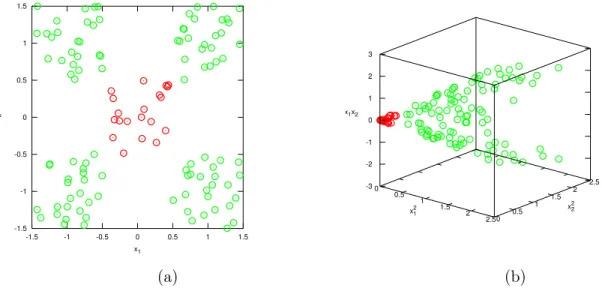
At this point it has been assumed that the feature set used is linearly separable; however this is not true in most of the cases. For example consider the features set in figure
3.6(a). There is not hyperplane capable to divide the feature set successfully. In those cases a nonlinear mapping φ :Rd→ F is applied, mapping the original features setS to a potentially much higher dimensional feature space F. Increasing the dimensionality of the feature space will increase the probability of a linear separation of the feature set. As an example, let the mapping functionφ be defined for the feature set in figure 3.6(a) as
φ(x) := (x2i, x2j, xixj) ∀ x= (xi, xj) (3.7) Figure3.6(b) shows the resulting feature space F. The feature space dimensionality has increased tod = 3 but now the feature set is easily separable using an hyperplane. Computing higher dimensional feature spaces provides a computational challenge due to the addition of complexity to the algorithm in real applications where the feature spaceF
can be highly dimensional. In such cases explicitly computing scalar product operations between elements within the feature space becomes unfeasible. In order to overcome this limitation the use ofkernel functions is widely extended.
3 Foundations 15
Figure 3.6: Feature space mapping using kernels. a) Original 2D data set not directly separable through an hyperplane. b) Mapped data set using φ(x) =z={x2
i, x2j, xixj}for x={xi, xj}.
k(xi,xj) = hφ(xi), φ(xj)i (3.8) so that there is not need to compute the mapping function φ(x) to calculate the scalar product between two feature points.
Different specific kernel functions have been defined such that (3.8) is met. Some of the most common kernels are shown in table 3.1[20]. The correct kernel function to use depends of the feature set and the final application.
Table 3.1: Common kernel functions used for SVM
Kernel Definition
16 3.4 Hu Moments in Image Processing
3.4.1
Geometric Moments
The geometric momentM of order (p+q) for a two-dimensional functionf(x, y) is defined as[19] tuples. In the case of digital images (3.9) is replaced by[13]
mpq =
The entire moments sequence {mpq}uniquely describes an image f(x, y) and in the same way, an image f(x, y) is uniquely determined by an specific moments sequence. However this fact requires the computation of an infinite number of moments which is impossible in practice. It is possible to select an specific subset of moments that describes in an unambiguous manner an image for a specific application.
The lower order moments describe a set of fundamental geometric properties of the image function f(x, y). Some of them are summarized in the table 3.2.
3.4.2
Moment Invariants
First introduced by Hu in [15], there are seven moment invariants or Hu moments useful to describe a two-dimensional image as follows:
3 Foundations 17
Table 3.2: Geometric properties of a two-dimensional digital image based on its moments
Property Definition Description
being the coordinates of the center of mass for a 2D im-age. The central moments of an image are invariant to translation. mass of an image with co-ordinates (¯x,y¯).
Orientations {m02, m11, m20}
Chapter 4
Recognition of Static Hand Poses
from a Top View
The main aim of this thesis is to identify a specific set of poses of a hand from a top view using depth images. Various visual features and classifiers are tested and its performance is compared.
This chapter presents the proposed system. Section 4.1 provides a general description of the algorithm implemented. Section 4.2 describes the data set used in the training process. A brief overview of the segmentation algorithm using RDF follows in Section
4.3. Section 4.4 introduces the visual features used for the pose classification stage and Section 4.5 provides a detailed description of the classifiers for pose recognition.
4.1
System Architecture
Figure 4.1 shows the general diagram of the system. The implementation is split in two processing phases:
1. PHASE 1: This phase is intended to the recognition of the hand and its main components (arm, palm and fingers) from a noisy environment such as a table with multiple objects. For this stage a modified version of Curfil [28] is used to train a random decision forest (RDF) based on depth images only. The resulting labeled blobs provide an estimation of the hand location and are feed to the next stage for the hand pose recognition.
20 4.2 The Data Set
Figure 4.1: General diagram of the system developed
Additionally the hand wrist is located as part of the process as a key point for further stages of hand pose analysis.
4.2
The Data Set
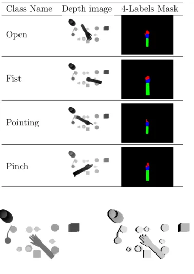
The dataset is based on a series of images synthetically generated simulating the Kinect© depth sensor. For this thesis four hand poses were used as shown in table 4.1. Alongside the depth information, ground truth masks are generated that label the arm (green), palm (blue) and the fingers (red).
The camera is set from a top view. In all training sets, several background objects are added to the scene in order to let the RDF identify the hand correctly among noisy ele-ments as shown in table4.1. The objects are randomly located within the scene removing any location constrains, i.e., objects within the scene can be closer to the front plane than the hand and can be partially occluded behind it. The scene sets the background plane at 1882 mm and the hand Z position varies from 900 mm to 1500 mm rotating in its XYZ dimensions in predefined ranges ensuring the generated poses are physically possible, leading to a total of 13728 images per class.
The images are rendered based on a model of LibHand [27] but modified to include objects in the background as well as shadows within the image.
Each hand is rendered with and without simulated IR shadow to allow the RDF to ignore the shadows caused by the displacement between the source of the IR pattern and the IR camera. Figure4.2 shows an example of the images generated.
4 Recognition of Static Hand Poses from a Top View 21
Table 4.1: Hand classes, depth image and ground truth masks Class Name Depth image 4-Labels Mask
Open
Fist
Pointing
Pinch
Figure 4.2: Generated depth image without shadow (left) and with shadows (right)
variants of the training set are generated: a first data set contains the synthetic images described above and the second has added noise in the depth images as encountered in the real depth sensors. The noise is added using the noise model given in [4] for Z dimension only as follows:
22 4.3 Phase 1: Pixel Segmentation using RDF
Table 4.2: Data sets (50% images with shadow)
Data Set # Noise (% images within the set) # Images per Class
1 100% 13728
2 0% 13728
3 50% 27456
4.3
Phase 1: Pixel Segmentation using RDF
In order to detect the hand in the data set a segmentation process is required. For this reason an RDF is used to learn the hand components in the training data and perform a per pixel classification process.
The training process is achieved using a modified version of Curfil[28], removing any dependencies to RGB information and using exclusively the depth images. Each tree is independently trained using breadth-first order. The feature implemented is based on the difference of the average value between two regions on the image in the neighborhood of the pixel that is being treated. Figure4.3 shows the feature calculation for a pixelq and offsets o1 and o2. Each region is defined by its wi and hi values corresponding to the width and height dimensions respectively.
1
o
q
o
2w
1h
1Figure 4.3: Example of Curfil’s feature calculation in a depth image
4 Recognition of Static Hand Poses from a Top View 23 parameters wi, hi normalized by the depth of the query pixeld(q) as follows:
Ri(q) :=R Curfil implements the information gain as its objective function for impurity estimation. The information gain is defined as the difference of Shannon entropy of the class distribu-tionDin the parent node and the weighted sum of Shannon entropies in class distribution in each child over the set of classes C[28] as follows
IC(D, DLEF T, DRIGHT) :=HC(D)−
|DLEF T|HC(DLEF T) +|DRIGHT|HC(DRIGHT)
|D|
(4.4) where the entropy over the classes HC for the current distribution D is defined as
HC(D) :=−
X
c∈C
p(c|D) log2(p(c|D)) (4.5)
Each tree is trained using randomly selected images from the data set, preserving the same class occurrence rate to avoid training bias.
The resulting RDFs generated from the training process are used to classify any incoming images and localize the hand and its components, such labeled images are feed to the next stage for the hand pose estimation.
4.4
Visual Features for Hand Pose Classification
In order to classify the labeled blob a set of visual features are extracted. Figure 4.4
shows the general preprocessing flow.
24 4.4 Visual Features for Hand Pose Classification
Hand mask Main axis
(rotation)
Figure 4.4: Features extraction process for hand pose classification
The hand position is then normalized by rotating its main axis at 90◦. The hand is always rotated with the fingers at the top of the image based on the colors histogram at the ends of the main axis.
Once the hand position is normalized, the next step computes the features for the classi-fication. Four features are used:
1. Entire mask labels histogram: The first feature corresponds to the labels his-togram of the entire blob based on the mask region, ignoring any information about background pixels:
Each bin cin the histogram h is calculated as the sum of all the pixels assigned to such class c in the points of the blob S. Two different values for the parameter N
are used for testing: N ∈ {1,P
c∈Ch(c)}.
2. Hand ROI histogram: For this feature additional information is extracted from the labeled images: the location of the hand’s wrist, found by the analysis of the main axis histogram and its boundary between the palm and the arm as shown in the figure 4.5.
4 Recognition of Static Hand Poses from a Top View 25
Wrist point Main axis
Figure 4.5: Location of the hand’s wrist
000
111
Wrist point
End of main axis
Hand ROI minor axis
1 std. dev.
Figure 4.6: Hand ROI for histogram calculation
Arm labels doesn’t provide any additional information about the shape of the hand since they belong to the arm itself which is independent of any hand’s pose. The background pixels on the other side provide information about the hand pose in a similar way to a convex hull calculation. This way the histogram is calculated as follows
h(c) = 1
N
X
i∈SR
pc(i) , c ∈C:={f ingers, palm, background} (4.10)
where SR corresponds to the points of all the pixels that belongs to the rectangular
26 4.4 Visual Features for Hand Pose Classification
1
3 4
2
Figure 4.7: Hand ROI quadrants for histogram calculation
of the hand pose on each quadrant independently, being able to capture discrimi-native patterns for each hand region.
Two variants of the feature are calculated for testing, the first one calculates a three element histogram for each quadrant qj, j ∈ {1,2,3,4} as follows:
where SQ corresponds to the points of all the pixels that belongs to the quadrant area and N =P
c∈Chqj(c).
The second variant of the feature unifies the background labels count into a single entry for the entire histogram, reducing the feature’s dimension from 12 to 9. This way the histogram calculation is expressed as
4. Hu Moments: Hu moments are used as features in a similar way than in [5] but considering each hand region independently. The first step is to separate the hand palm and fingers regions from the rotated image as shown in figure 4.8. The hand regions are extracted using a region growing algorithm and then passed to the Hu calculator.
4 Recognition of Static Hand Poses from a Top View 27
Rotated hand
Fingers (red label)
Palm (blue label)
Hu Moments
calculator
calculator Hu Moments
Figure 4.8: Hand regions extraction and Hu moments calculation from rotated image Table 4.3: Features for hand pose classification
# Feature # dimensions
1 Full image histogram 3
2 ROI histogram 3
3 ROI histogram (denormalized) 3
4 ROI quadrants histogram 12
5 ROI quadrants histogram (reduced) 9
6 Hu moments 14
4.5
Phase 2: Gesture Classification
Chapter 5
Experimental results
In this chapter a set of experimental results on the proposed system are shown. Section5.1
describes the different data sets used in the experiments. Section5.2 provides a summary of the segmentation results produced by the RDF classifier in the first stage of the system. A brief analysis of the wrist location results is provided in section 5.3 as a key point for further stages of the system. Finally, section5.4 provides a detailed analysis of the results from the second stage of the system, aimed to the classification of the hand pose. An RDF classifier is tested and its prediction capability is compared against a classic SVM classifier. At last, the RDF classifier for pose estimation is exposed to ideally labeled hand blobs in order to determinate the classification performance of the second stage assuming an ideal segmentation.
5.1
Data set
The generation process of the data set in use was provided in chapter4.2. The experiments along this chapter are based on a set of three different data sets presented in section 4.2
and shown in table 5.1 for convenience. Each data set differs on the amount of images with noise within the entire set. All data sets contain images rendered with shadows and without them, to improve shadows immunity. A total of 4 hand poses are used: open, pointing, fist and pinch, as depicted in table 5.2 for several rendering location/rotation variations.
Table 5.1: Data sets used for experimental results (50% images with shadow) Data Set # Noise (% images within the set) # Images per Class
30 5.2 Segmentation of Hand Regions
set used on each experiment.
Table 5.2: Hand pose samples at different location/rotation values
Class Name Sample 1 Sample 2 Sample 3 Sample 4 Sample 5
Open
Fist
Pointing
Pinch
A total of 10000 randomly selected images from each data set are used to train the first stage of the system aimed to the hand segmentation. An additional batch of 10000 are then used for testing that stage and feed to the hand pose classification stage to train the RDF and SVM classifiers. Finally a 5000 images set is used to validate the classifiers of such stage.
5.2
Segmentation of Hand Regions
This section presents a set of experimental results aimed to the analysis of the hand segmentation stage of the system presented in section 4.3. Three RDF classifiers are trained with the data sets introduced in section 5.1 in order to validate the effect of the noise within the training images. These results correspond to the classification output for each individual pixel, where no information of neighbor classifications is taken into account. Furthermore, detailed analysis on the prediction capabilities of the RDF is performed.
Each RDF is trained with the set of parameters listed in table 5.3. No parameters optimization has been performed since such topic is out of the temporal scope of this thesis.
The classifiers are identified as follows:
5 Experimental results 31
Table 5.3: RDF configuration for hand segmentation
Parameter Value
Feature max box edge size (region size) 10 Feature max box offset (box radius) 30
Train set size 10000
Test set size 10000
• RDF B: RDF trained with data set 2, specially focused on the effect of noise in the prediction capability.
• RDF C: RDF trained with data set 3. This test is aimed to test the effect of training the classifier with samples with noise and without noise.
The accuracy of each classifier has been measured quantitatively and summarized in tables
5.4, 5.5 and 5.6, which correspond to the confusion matrices for the classifiers A, B and C respectively. C0, C1, C2 and C3 are the background, fingers, arm and palm classes,
respectively. The prediction results between the three random forests is very similar, with only a maximum variation of 7% around the mean. Since the background pixels comprise the majority of the region on each blob its accuracy in each matrix is near the 100%; however the classification of the pixels belonging to the hand parts presents more confusion, being the fingers the class with the larger confusion, classifying around 46% of the samples as background and palm.
Table 5.4: Confusion matrix for RDF A trained with depth images without noise. (Data set size = 10000 with 0% images without noise )
Predictions Confussion
Matrix C0 C1 C2 C3
32 5.2 Segmentation of Hand Regions
Table 5.5: Confusion matrix for RDF B trained with noisy depth images. (Data set size = 10000 with 100% images with noise)
Predictions Confussion
Matrix C0 C1 C2 C3
C0 0.997 0.001 0.002 0.000 C1 0.191 0.473 0.037 0.300 C2 0.076 0.002 0.904 0.018 Classes
C3 0.073 0.028 0.054 0.845
Table 5.6: Confusion matrix for RDF C trained with mixed depth images. (Data set size = 10000 with 100% images with noise)
Predictions Confussion
Matrix C0 C1 C2 C3
C0 0.997 0.001 0.002 0.000 C1 0.197 0.513 0.030 0.261 C2 0.080 0.004 0.897 0.019 Classes
C3 0.077 0.041 0.043 0.839
of the confusion matrix[24] and omitting thebackground predictions leads to the results in table 5.7 for the accuracy rates for the classes C1, C2 and C3 and the total per-class
accuracy. It is possible to notice an slight reduction in the prediction accuracy when noise is injected, decreasing in up to 4.6% the average prediction for the classifier B and 2.8% for the classifier C.
Table 5.7: Class accuracy omitting background class prediction statistics Classifier C1 accuracy C2 accuracy C3 accuracy Average accuracy
A 0.680 0.984 0.930 0.865
B 0.584 0.978 0.912 0.825
C 0.638 0.975 0.910 0.841
The average classification accuracy for arm is 97.9% and 91.7% for the palm, being the fingers the class with the lower average prediction with 63.4%, which coincides with the results obtained from the confusion matrices. The fingers class presents its lower prediction accuracy for the RDF B with 58.4%.
Two interesting results are obtained from the confusion matrices in tables5.4,5.5and5.6
5 Experimental results 33
Second, the better accuracy of the RDF C compared with the RDF B. Training the RDF with 50% of noisy images helped the forest to increase its accuracy in around 1.8%, improving the RDF immunity to the noise.
Since the RDF C presents the best average accuracy with noisy images, improving con-siderably the pixel prediction for the fingers, it is selected as the reference classifier along the remaining sections of this thesis.
Table 5.8 shows an example of the prediction results for each classifier.
Table 5.8: Experimental hand segmentation results for RDF A, B and C (Using training parameters from table 5.3 )
Class Name Depth image Ideal
prediction RDF A RDF B RDF C
Open
Fist
Pointing
Pinch
5.3
Wrist Location
One of the key processing stages within the system is the estimation of the wrist point in the labeled blobs provided by the segmentation phase.
34 5.3 Wrist Location
difference between the ideal and estimated wrist points lies within a circle with center (xideal, yideal) and with radius σarmminor.
Table5.9 shows the relative wrist distance measurements for each class and for the entire data set, providing the mean and standard deviation. Additionally, the percentage of samples with a relative wrist distance lower than 1 is provided. The average mean relative distance is 0.509 with standard deviation values around 0.337, this means that most of the wrist points calculated provide a good estimation of the real wrist point location. This result is confirmed by looking at the percentage of samples within the radius σarmminor
which in average corresponds to 93.63%.
Table 5.9: Relative wrist point distance measurements for RDF predicted images (Data set size = 10000)
Measument Open Pointing Fist Pinch Average
Mean 0.517 0.508 0.501 0.509 0.509
Std. Dev. 0.366 0.315 0.336 0.330 0.337
Samples within radius (%) 92.84 93.56 94.48 93.64 93.63
In order to determinate whether the wrist estimation is out of the hand region, the relative distance has been calculated for thexand ycoordinates separately as listed in table5.10. The x coordinates have an average relative distance of 0.284 with 99.95% of the samples within the radius. In the other hand theycoordinates present an average relative distance of 0.426 with 94.32% of the samples within the radius.
Table 5.10: Relative wrist point distance forxandycoordinates (Data set size = 10000) Measument Open Pointing Fist Pinch Average
Mean X 0.272 0.289 0.284 0.292 0.284
Std. Dev. X 0.198 0.216 0.199 0.202 0.204
% Samples Rel∆X <1 100 99.86 100 99.95 99.95
Mean Y 0.449 0.425 0.421 0.411 0.426
Std. Dev. Y 0.389 0.328 0.357 0.357 0.359
% Samples Rel∆Y <1 93.35 94.67 94.77 94.49 94.32
5 Experimental results 35
5.4
Hand Pose Classification
This section presents the analysis of the hand pose classification stage of the system. The RDF and SVM classifiers are tested and their performance is discussed alongside with the experimental results.
The features used for the hand pose estimation are listed in table 5.11 (for more details about their definition see section 4.4). Feature 7 has been included for analysis purposes and it is composed as the union of all the previous features, the main goal of this feature is to evaluate the discriminatory capabilities of each classifier among all the range of possible features to use.
Table 5.11: Experimental visual features used for hand pose classification
# Feature # dimensions
1 Full image histogram 3
2 ROI histogram 3
3 ROI histogram (denormalized) 3
4 ROI quadrants histogram 12
5 ROI quadrants histogram (reduced) 9
6 Hu moments 14
7 Complete feature set 45
5.4.1
Classification Using RDF
The training parameters used for the RDF are shown in table 5.12.
Table 5.12: RDF configuration used for hand pose classification
Parameter Value
Max depth [10,25]
36 5.4 Hand Pose Classification
lower classification error, close to 10%. The ROI quadrants histogram and its option with dimensions reduced present a classification error close to 20%, being it the isolated feature that provide best classification results. On the other hand the Hu moments provide the worst classification error for all the RDF configurations.
0
Hand pose classification error for different RDF configurations
All features
Figure 5.1: Classification error vs RDF configuration for different features
Table 5.13 shows the minimum classification error (i.e. the maximum average per-class accuracy) for each feature and the corresponding depth and size values. The best result is emphasized with a gray shadow, provided by the entire set of features using an RDF of depth 15 and size 150, with an average per-class accuracy of 91%.
Table 5.13: Best classification error and average per-class accuracy using all features
Feature RDF Depth RDF Size (trees) Min. Classifica-tion Error (%)
Average Per-class accuracy
All Features 15 150 8.680 0.91
General histogram 15 110 30.280 0.70
ROI Quadrants hist. (red.) 25 90 16.720 0.83
ROI Quadrants hist. 25 140 15.960 0.84
ROI hist. (denormalized) 15 100 34.060 0.66
ROI histogram 15 100 37.760 0.62
5 Experimental results 37
Figure5.2shows the classification error curves for the RDF trained with the entire features set at a constant depth value and varying the RDF size. Depth values above 15 levels behave in a similar way with a minimum classification error around 8.87%. This fact is presented in more detail in table 5.14 which presents the best classification error and average per-class accuracy values for each RDF depth. For depth values above 15 levels the best average per-class accuracy is 91% and it only varies on the number of trees used.
8 9 10 11 12 13 14
0 50 100 150 200
Classification Error (%)
RDF Size (trees)
Hand pose classification error vs RDF size
Depth = 10 Depth = 15 Depth = 20 Depth = 25
Figure 5.2: Classification error vs RDF size for different depth values using the entire features set
Table 5.14: Best classification error and average per-class accuracy using all features RDF Depth RDF Size (trees) Min. Classification Error (%) Average Per-class accuracy
10 90 10.040 0.90
15 150 8.680 0.91
38 5.4 Hand Pose Classification
among the others. Additionally, fist and pinch classes present an accuracy rate higher than 91% leaving the pointing class at last with 84%. As it is expected the pinch and pointing classes present a mutual confusion of around 7% due to their physical similarity. An interesting result is the confusion presented between the pointing and fist labels, probably caused by the misclassification of the index finger pixels, leading to a segmented blob similar to a fist, as shown in the experimental results in figure 5.3. Despite the segmentation of the blob in figure5.3a) provides a correct pixel assignment for the index finger, in the figure 5.3 b) the index pixels were classified to thearm class which leads to a poor set of visual descriptors for the pose estimator.
Table 5.15: Confusion matrix for hand classification using the complete set of features (depth = 25, RDF size = 130)
Predictions Confussion
Matrix Open Pointing Fist Pinch
Open 0.968 0.013 0.00 0.019
Pointing 0.008 0.839 0.081 0.072 Fist 0.002 0.074 0.918 0.007 Classes
Pinch 0013 0.070 0.002 0.916
(a) (b)
Figure 5.3: Misclassification of pointing class pixels. a) Index finger correctly segmented. b) Index finger misclassified pixels
Similar to boosting, random decision forests provide useful information about the im-portance of each feature component within the training process. This is a interesting feature commonly used to select and reduce the size of a feature set. Table5.16 provides a summary of the features importance rates obtained from the RDF analysed. Features based on the ROI quadrants analysis presents the higher importance percentage within the range of 23-33%. Features such as the Hu moments with 14 components provides only a 9.501% of importance, with 10 components with a 0%; being the first moment for palm and the first and second moments for the fingers the ones with higher importance. Additionally, in all the histogram based features thefinger component provides the higher percentage of information for the pose classification, which can be related to the fact that this visual feature is the most dynamic between different hand postures.
5 Experimental results 39
used to reduce the size of the feature set, removing all the components that provide 0% of information or close and just computing the main components.
Table 5.16: Features importance percentage for an RDF trained with all the features sets (depth = 15, size = 120)
In the next section SVM classification is analysed in order provide a comparison point of the result presented with a classic ensemble.
5.4.2
Classification Using SVM
40 5.4 Hand Pose Classification
Table 5.17: Parameters range used for SVM grid analysis Parameter Range
γ [0.1, 0.0002]
C [1, 2000000]
Table 5.18 summarizes the classification error and average per-class accuracy for each feature. As expected from the result obtained from the RDF analysis, the SVM presented the best classification accuracy when the entire set of features is used as input to the classifier. However, classification accuracy is much lower for the SVM than the obtained using RDF with a minimum classification error of 24.94%. It is interesting to see how the Hu moments present the worst classification accuracy among the features set, coinciding with the results obtained for the RDF classifier.
Table 5.18: Classification error and average per-class accuracy for SVM classifier (γ = 0.0001,C = 5.275)
ROI Quadrants hist. (red.) 50.14 0.50
ROI Quadrants hist. 50.08 0.50
ROI hist. (denormalized) 39.26 0.61
ROI histogram 56.96 0.43
Hu Moments 72.28 0.28
5.4.3
Classification of Ideal Predicted Blobs using RDF
It has been demonstrated the superiority of the random forests for the hand pose classi-fication compared with support vector machines classifiers, for the features set proposed. In this section it is analysed the classification capability of the proposed features using random forests and an ideal set of predicted blob labels. Separating the hand blob segmen-tation error from the classification process allows to measure the prediction capabilities of the system in a controlled environment.
The RDF is trained with the same parameters shown in table5.12 for each of the features proposed. Figure 5.4 depicts the classification error based on different depth and size settings for the RDF on each feature. In contrast with the results obtained in figure
5.1, all the features but the Hu moments got a classification error under 5%. Table 5.19
5 Experimental results 41
forests presented an average per-class accuracy above 90% with the Hu moments based RDF being the less accurate with 91%.
0
Hand pose classification error for different RDF configurations
All features
Figure 5.4: Classification error vs RDF configuration for different features with ideal segmentation of hand blobs
Table 5.19: Best classification error and average per-class accuracy using all features
Feature RDF Depth RDF Size (trees) Min. Classifica-tion Error (%)
Average Per-class accuracy
All Features 15 100 0.00 1.00
General histogram 20 110 0.090 1.00
ROI Quadrants hist. (red.) 20 100 0.000 1.00
ROI Quadrants hist. 20 100 0.000 1.00
ROI hist. (denormalized) 25 120 0.510 0.99
ROI histogram 25 130 0.400 1.00
42 5.4 Hand Pose Classification
Table 5.20: Features importance percentage for an RDF trained with all the features sets with ideal segmentation (depth = 15, size = 100)
Feature Component
Chapter 6
Conclusions
This thesis presents a two staged architecture for the hand pose recognition of four hand postures (open, pointing, fist and pinch), using depth images in a top view perspective without any color information. The proposed design removes some of the classic constrains in hand recognition with depth sensors such as the hand relative position to other objects and verticality with respect to the camera. Additionally the proposed solution addresses some common error sources in IR sensors such as Gaussian noise and shadows.
Along the entire project a synthetic data set was used to perform the training and verifi-cation test. Such data set was generated based on LibHand hand model[27] and allowed the analysis of various characteristics of depth images independently, such as the effect of the depth noise in the training process.
The first processing stage was implemented using a modified version of Curfil[28] to train an RDF for per-pixel classification, identifying the arm, palm and fingers in the depth images. It was found that the addition of Gaussian noise in the depth images (based on Kinect’s noise model[4] for Z direction) causes a decrement of just 4.6% in the classification accuracy, exposing a high level of immunity to Gaussian noise. Also, using a combination of depth images with 50% of the samples with noise for training increments the pixel classification accuracy of the RDF in about 1.8%, increasing the RDF immunity to noise. It was possible to get a classification accuracy for the segmentation stage up to 84.1%, being the fingers the most difficult region to estimate with a 26% of confusion with the palm.
44 6.1 Future Work
was proved the higher capability of the random forests to learn from a set of features and provide an acceptable prediction rate compared with SVM, providing up to a 91% of average per-class accuracy against 75% of the SVM. Additionally it was demonstrated that pixel based features calculated from the ROI quadrants around the hand provide the higher discriminative information in the classification process. The Hu moments of the palm and fingers provide the lowers discriminative information presenting meaningful metrics only on their first and second moments.
In general it has been proved the capability of random decision forests for hand pose classification from depth images where no hand location constrains or color information is used. Additionally it has been possible to identify a set of simple visual features that provide high discriminatory information for hand pose estimation for hand blobs.
6.1
Future Work
It is left for future work to test the proposed solution under real conditions using real depth images for the prediction process. On the other hand, the major disadvantage of RDF is the required training times, which considerably limit the amount of points in the parameter space that can be explored. Tuning of such parameters is a task still to be performed to optimize the results obtained. Additionally, other RDF ensembles variants can be used in order to improve the classification accuracy and overall performance, such as the usage of multi-layered random forests (MLRF)[18] that improves memory usage and speed.
Bibliography
[1] OpenNI. URL http://www.openni.org.
[2] Dustin Boswell. Introduction to Support Vector Machines. pages 1–15, 2002. URL
http://videolectures.net/epsrcws08_campbell_isvm/.
[3] CR Cameron. Hand tracking and visualization in a virtual reality simulation. (SIEDS), 2011 IEEE, 22904:127–132, 2011. URL http://ieeexplore.ieee.org/
xpls/abs_all.jsp?arnumber=5876867.
[4] Benjamin Choo, Michael Landau, Michael DeVore, and Peter Beling. Statistical Analysis-Based Error Models for the Microsoft KinectTM Depth Sensor. Sensors, 14(9):17430–17450, 2014. URL http://www.mdpi.com/1424-8220/14/9/17430/. [5] S Conseil, S Bourennane, and L Martin. Comparison of Fourier Descriptors and Hu
Moments for Hand Posture Recognition . EURASIP, page 20, 2007.
[6] A. Criminisi and J. Shotton. Decision Forests for Computer Vision and Medical Image Analysis. 2013.
[7] Arnaud Dapogny, Raoul De Charette, and Sotiris Manitsaris. Towards a Hand Skeletal Model for Depth Images Applied to Capture Music-like Finger Gestures. 10th Int. Symposium on Computer Music Multidisciplinary Research (CMMR’2013), 2013. URL http://hal-ensmp.archives-ouvertes.fr/hal-00875721$\
delimiter"026E30F$nhttp://hal.archives-ouvertes.fr/hal-00875721/.
[8] Martin de La Gorce, David J Fleet, and Nikos Paragios. Model-Based 3D Hand Pose Estimation from Monocular Video. IEEE transactions on pattern analysis and machine intelligence, 33(9):1793–1805, February 2011. URLhttp://www.ncbi.nlm.
nih.gov/pubmed/21339527.
46 Bibliography
[11] Ali Erol, George Bebis, Mircea Nicolescu, Richard D. Boyle, and Xan-der Twombly. Vision-based hand pose estimation: A review. Computer Vision and Image Understanding, 108(1-2):52–73, October 2007. URL
http://linkinghub.elsevier.com/retrieve/pii/S1077314206002281http: //citeseerx.ist.psu.edu/viewdoc/download?doi=10.1.1.76.6351&rep=
rep1&type=pdf.
[12] Yoav Freund, Robert E Schapire, Park Avenue, and Florham Park. A Short Intro-duction to Boosting. 14(5):771–780, 1999.
[13] Rafael C. Gonzalez and Richard E. Woods. Digital Image Processing (3rd Edition). Prentice-Hall, Inc., Upper Saddle River, NJ, USA, 2006.
[14] Trevor Hastie, Robert Tibshirani, and Jerome Friedman. The Elements of Statistical Learning. Springer Series in Statistics. Springer New York Inc., 2001.
[15] Ming-Kuei Hu. Visual pattern recognition by moment invariants. Information The-ory, IRE Transactions on, 8(2):179–187, 1962.
[16] Christian Igel. Machine Learning: Kernel-based Methods. pages 21–23, 2014. URL
http://image.diku.dk/igel/teaching/KernelBasedMachineLearning.pdf.
[17] Cem Keskin, Furkan Kırac, Yunus Emre Kara, and Lale Akarun. Real Time Hand Pose Estimation using Depth Sensors. IEEE International Conference on Computer Vision Workshops, pages 1228–1234, 2011.
[18] Alina Kuznetsova, Laura Leal-Taixe, and Bodo Rosenhahn. Real-Time Sign Lan-guage Recognition Using a Consumer Depth Camera. 2013 IEEE International Conference on Computer Vision Workshops, pages 83–90, December 2013. URL
http://ieeexplore.ieee.org/lpdocs/epic03/wrapper.htm?arnumber=6755883.
[19] Simon Xinmeng Liao. Image Analysis by Moments. Technical report, University of Manitoba, 1993.
[20] Klaus Robert M¨uller, Sebastian Mika, Gunnar R¨atsch, Koji Tsuda, and Bernhard Sch¨olkopf. IEEE Transactions on Neural Networks.
[21] Iason Oikonomidis, Nikolaos Kyriazis, and Antonis Argyros. Efficient model-based 3D tracking of hand articulations using Kinect. Procedings of the British Machine Vision Conference 2011, pages 101.1–101.11, 2011. URL http://www.bmva. org/bmvc/2011/proceedings/paper101/index.htmlhttp://www.researchgate. net/publication/233950932_Efficient_model-based_3D_tracking_of_hand_
articulations_using_Kinect/file/9fcfd50d72d96c01ca.pdf.
Bibliography 47
[23] Zhou Ren, Junsong Yuan, and Zhengyou Zhang. Robust hand gesture recognition based on finger-earth mover’s distance with a commodity depth camera. Proceedings of the 19th ACM international conference on Multimedia - MM ’11, page 1093, 2011.
URL http://dl.acm.org/citation.cfm?doid=2072298.2071946.
[24] By Jamie Shotton, Toby Sharp, Alex Kipman, Andrew Fitzgibbon, Mark Finocchio, Andrew Blake, Mat Cook, and Richard Moore. Real-Time Human Pose Recognition in Parts from Single Depth Images. 2011.
[25] Jamie Shotton, Andrew Fitzgibbon, Mat Cook, Toby Sharp, Mark Finocchio, Richard Moore, Alex Kipman, and Andrew Blake. Real-time human pose recog-nition in parts from a single depth image. In CVPR. IEEE, June 2011. URL
http://research.microsoft.com/apps/pubs/default.aspx?id=145347.
[26] Danhang Tang, Tae-kyun Kim, and Tsz-Ho Yu. Real-time Articulated Hand Pose Estimation using Semi-supervised Transductive Regression Forests. 2013.
[27] Marin ˇSari´c. Libhand: A library for hand articulation, 2011. URL http://www.
libhand.org/. Version 0.9.
[28] Benedikt Waldvogel. Accelerating Random Forest on CPUs and GPUs for Object-Class Image Segmentation. PhD thesis, 2013.