A multilevel decomposition of school performance using robust nonparametric frontier techniques

Texto completo

(1)A mutilevel decomposition of school performance using robust nonparametric frontier techniques. Claudio Thieme. Diego Prior. Emili Tortosa-Ausina. Universidad Diego Portales. Universitat Autònoma de Barcelona. Universitat Jaume I and Ivie. ∗. and IESEG School of Management. August 28, 2012. Abstract We propose a methodology for evaluating educational performance, from a multilevel perspective. We use partial frontier approaches to mitigate the influence of outliers and the curse of dimensionality. Our estimation considers idiosyncratic variables at the school, class, and student levels. Our model is applied to a sample of students in fourth year of primary school in urban schools in Chile. Results are in line with previous findings that less than 30% of the variance in students’ educational attainment is attributable to their schools. Results also corroborate that a model considering only student-level variables yields high inefficiencies not attributable to school management, but rather to inadequate resource-endowment policy. Therefore, when disregarding specific variables concerning the resources allocated to the schools, the performance of those schools is undervalued, largely because inefficiencies caused by suboptimal resource endowments or difficulties arising from the socioeconomic environment are instead attributed to poor school management.. Key words and phrases: efficiency, multilevel analysis, order-m, school effectiveness. JEL Classifications: C61, H52, I21. Communications to: Emili Tortosa-Ausina, Departament d’Economia, Universitat Jaume I, Campus del Riu Sec, 12071 Castelló de la Plana, Spain. Tel.: +34 964387168, fax: +34 964728591, e-mail: [email protected].. ∗ Claudio Thieme acknowledges the financial support of Fondo Nacional de Desarrollo Científico y Tecnológico (FONDECYT), grant #11085061. Diego Prior and Emili Tortosa-Ausina acknowledge the financial support of Ministerio de Ciencia e Innovación (ECO2010-18967/ECON and ECO2011-27227/ECON). Emili Tortosa-Ausina also acknowledges the financial support of Generalitat Valenciana (PROMETEO/2009/066). All three authors are grateful for the comments of the two referees. The usual disclaimer applies..

(2) 1.. Introduction. Over the last 20 years, there has been growing interest among academics and policy-makers alike visà-vis school effectiveness research. The central hypothesis of these research initiatives postulates that certain characteristics of a school under analysis can impact its students’ educational attainment, and that this impact holds even after controlling for the students’ socioeconomic, academic, and demographic characteristics (Goldstein and Woodhouse, 2000; Opdenakker and Van Damme, 2001; Phillips, 1997; Sammons et al., 1997; Bosker and Witziers, 1996). There has been remarkable methodological progress in this line of research, mostly due to the development of multilevel models (Bryk and Raudenbush, 2002; Goldstein, 1995) that have improved both the definition and measurement of the underlying causes of students’ learning processes (Aitkin and Longford, 1986). The general consensus is that students’ educational attainment depends on both their personal circumstances and on the idiosyncratic characteristics of their schools and those schools’ catchment areas. In order to model these scenarios, the different levels are considered as hierarchical systems of the students and schools; in these, individuals and groups are stratified into different clusters, using variables defined for each of these levels (Hox, 2002). This progress in the field has facilitated the resolution of one of the main methodological problems faced by pioneering studies—namely, the inability to decompose the variety of nested effects that explain students’ educational achievements. The new methodological proposals enable one to ascertain the share of each student’s educational attainment that can be attributed to the various variables measured at different levels (i.e., student, class, school, and district); this constitutes information relevant to the design of specific policy measures at each level—i.e., student, school, and environment—thus improving service delivery in this sector. Students’ educational attainment is usually measured by using common test scores from all schools, whereas the average result of the tests for a given school is assumed to be an indicator of its educational attainment. The variance among schools with respect to total variance (i.e., among all students at different schools) is defined as the “gross effect” of the school. In contrast, the variance within a school, which cannot be explained by control variables specific to each school (such as, for instance, the level of resources endowed by the government or the average socioeconomic level of the students) is considered the “net effect” of the school. It is expected that a significant proportion of within-school variance can be explained by factors specific to each school. The results of the multilevel studies available thus far indicate that the most important effect is the variance among students that can be attributed to their individual characteristics. Additionally, the school effect, once the socioeconomic level of the students has been controlled for, ranges between 10% and 30%; it is higher in mathematics than in either languages or science, and it is also higher in primary education than in secondary education (Cervini, 2009; Murillo, 2010; Blanco, 2010). Part of this literature also indicates that the educational and socioeconomic characteristics of the students explain not only the. 1.

(3) differences in the educational attainment of students within a school, but also among schools. In some countries, this would be related to the schools’ selection, on educational and socioeconomic bases, of their students (see, for instance, Elacqua et al., 2006). In our model we also control for two important effects considered in the literature, namely, the peer effects on student achievement (see, for instance McEwan, 2003) and the selection bias (see, for instance McEwan, 2001; Mizala and Torche, 2012). Both effects are important in the Latin American context as shown by Somers et al. (2004) who found that, after controlling for peer and selection effects, the extra educational achievement obtained by private schools compared with public schools was negligible (in a more general context, see Waslander et al., 2010). With particular regard to the selection bias effect, according to which there are unobservables such as students’ ability, motivation or ambition that should not be confounded with the relative effectiveness of the schools, the literature is increasing rapidly in the case of Chile, as shown by some recent studies such as Lara et al. (2011) or Mizala and Torche (2012) which account for this issue. Most of the research initiatives used to measure school efficiency have been developed in the fields of education and economics. One of the techniques that have been used more intensely therein is regression analysis. However, as indicated by Silva Portela and Thanassoulis (2001), regression equations “do not explore the variation in pupils’ outcomes inside the same school as this variation is hidden behind an average”. Although these concerns were also raised by Goldstein (1997), who provides an example warning of the possibly misleading nature of an aggregate-level analysis, the variation hidden behind an average was a limitation of the “early attempts” to relate achievement and school factors (Goldstein, 1997, p.386). In addition, as indicated by De Witte et al. (2010), school data are usually nested (e.g., students within classes, classes within schools, schools within districts, districts within local education authorities, etc.) and, in such a case, the parametric ordinary least squares (OLS) estimates can be biased, in that the presence of intra (or within) unit correlation can lead to underestimations of the standard error of the regression coefficients (De Witte et al., 2010, p.1224). In addition, the variables selection within this approach is usually restricted to only one output. In contrast, over the last few years some methods have been used that, among other advantages, allow for an extension of the bundle of outputs and inputs. Most of these methods have been developed in the field of efficiency and productivity measurement using frontier techniques; among them, Data Envelopment Analysis (DEA) stands out on the basis of both the number and relevance of applications.1 DEA is a linear programming technique initially developed by Charnes et al. (1978) to measure the productive efficiency of the so-called decision-making units (DMUs). It has been extensively applied to assess of efficiency in many types of DMUs, including banks, retail outlets, municipalities, hospitals, and schools, to name just a few. Some of its most valued virtues are that it neither stipulates a functional form for the cost (or profit, or revenue) functions, nor for the distribution of efficiencies; it therefore 1 Among. nonparametric methods, DEA is the most popular technique used to measure efficiency while using frontier techniques, whereas SFA (Stochastic Frontier Analysis) is the most popular within the parametric field. See Fried et al. (1993) and Fried et al. (2008) for interesting panoramas of both branches of research within frontier efficiency analysis.. 2.

(4) closely envelops the data. The existing literature is sizeable, but the unfamiliarized reader can become acquainted by reviewing the recent surveys of Emrouznejad et al. (2008) or Cook and Seiford (2009), for instance. In addition to allowing for the simultaneous modeling of several inputs and outputs, DEA also has another appealing feature: it allows for comparisons of each unit with optimal or efficient values, since it is based on estimations of an efficient frontier where best-practice DMUs lie. DEA also has a variant—the Free Disposal Hull (FDH) (Deprins et al., 1984)—which differs from DEA in its removal of the convexity assumption. In practical terms, this implies that each DMU is compared only to other existing DMUs, and that it cannot be evaluated against convex combinations of efficient units. Therefore, FDH is even more flexible than DEA, since there are even fewer required assumptions. In the field of education, several studies have applied these techniques in order to assess different aspects related to school efficiency. Some interesting literature contributions that use DEA to consider school-level data include Bessent et al. (1982), Ruggiero et al. (1995), Mancebón and Mar Molinero (2000), Bifulco and Bretschneider (2001), Mizala et al. (2002), and Ouellette and Vierstraete (2005). Far fewer students use FDH and include, among others, Oliveira and Santos (2005). Studies using student-level data in DEA assessments are more recent, starting with Thanssoulis (1999). Silva Portela and Thanassoulis (2001) have made substantial methodological progress by proposing a DEA approach that identifies the sources of student under-attainment including, among other factors, school effectiveness, or the type of funding regime under which the school operates. Their variable-returns-to-scale (VRS) DEA model measures student efficiency while considering a global frontier (student-within-all-schools-efficiency) and local frontiers specific to each school (student-within-schoolefficiency). The distance to the local frontier corresponds to the student effect, whereas the distance between the local and global frontiers reflects the school effect. Followers of this approach include Thanassoulis and Silva Portela (2002), Silva Portela and Camanho (2010), and Mancebón and Muñiz (2007), among others. In this paper, we extend the methods of Silva Portela and Thanassoulis (2001) in several directions. Whereas Silva Portela and Thanassoulis (2001) and many of their followers use either DEA or FDH, we exploit some alternative new concepts of efficiency, as well as new nonparametric estimators. Specifically, we base our analysis on the order-m partial frontiers described by Cazals et al. (2002), which offer several advantages over previously used efficiency estimation methods. Although compared to parametric methods DEA and FDH have the significant advantage of not imposing a particular functional form on the relationship between production inputs and outputs, they do have some drawbacks. As indicated by Cazals et al. (2002), Simar (2003), Simar and Wilson (2008), and Wheelock and Wilson (2009), both DEA and FDH are highly sensitive to extreme values and noise in the data, and suffer from the well-known curse of dimensionality (Simar and Wilson, 2008). In contrast, order-m estimators √ are robust with respect to extreme values and noise, and are n consistent: they do not suffer from the curse of dimensionality. In the field of education, only De Witte et al. (2010) consider the use of order-m estimators; however, they do not consider explicitly multilevel models, as we do. Specifically,. 3.

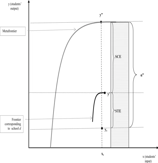
(5) we include school-level variables that refer to controllable and noncontrollable inputs for each school. In the current study, we also combine the application of partial order-m frontiers with the concept of the “metafrontier” (Battese et al., 2004; O’Donnell et al., 2008)—one that is especially helpful when working with observations that are stratified into different levels and can be evaluated using different frontiers. In addition, with respect to the work of Silva Portela and Thanassoulis (2001), we extend the analysis to include contextual variables, at both the student level and the school level. Moreover, we also provide a relevant application that focuses on the case of Chile, a country that has taken serious initiatives to improve public service delivery, especially in such important areas as the provision of educational choice, incentives, and information. As indicated by Mizala et al. (2007), among these initiatives, a critical input is an assessment of school performance, which includes in several cases a ranking of the institutions that is to be used, as required, to inform parents or to allocate rewards (or penalties) in accountability-type schemes; such instruments are also used in other countries, including the United States. In this regard, the partial frontiers that we use will yield a more precise ranking of schools, thus improving the informativeness of either DEA or FDH. In our particular application, the data from the Chilean educational system consist of a sample of 11,319 students studying in the fourth year of primary school, corresponding to 176 elementary-level urban schools. To present and discuss our proposal, the rest of this paper is organized as follows. Section 2 presents the model and methods, section 3 describes the data, and section 4 discusses the results. Finally, section 5 provides concluding remarks.. 2.. An order-m multilevel frontier proposal. 2.1. The decomposition of the multilevel frontier model The immediate antecedent of our proposal is the study by Thanassoulis and Silva Portela (2002). These authors consider two frontiers: the local frontier, specific to each school oriented to an estimation of student-within-school efficiency; and the global frontier, used to estimate student-within-all-schools efficiency. The distance to the local frontier depends on the student’s efficiency (the so-called student effect, henceforth STE), whereas the distance separating the local and the global frontiers expresses the school efficiency (the so-called school effect, or SCE). Figure 1 documents the rationale that generates these two effects. Student (c) under analysis obtains the output level represented by y c , which has the input level xc . When comparing the academic performance of this student to the local frontier (i.e., that corresponding to school d where student c is enrolled), it is obvious that student c is inefficient, as on the frontier we find more-efficient students who attend the same school and obtain better results (y ′ ) with the same level of inputs (xc ). Accordingly, the student effect (the student-within-school efficiency, to use the term coined by Thanassoulis and Silva Portela (2002)) can be determined as a ratio: the potential output divided by the actual output (STE = α′ = y′ /yc ). The student effect is higher than unity when. 4.

(6) the student is inefficient (as in the case presented in Figure 1), and equal to unity otherwise. When compared to the overall frontier (metafrontier or the student-within-all-schools efficiency, terms used by Thanassoulis and Silva Portela (2002)), the efficiency coefficient for the student under analysis is OE = α” = y ′′ /yc . Having these two reference frontiers, the school effect (a sort of technology-gap ratio separating the school-specific frontier from the overall frontier) is determined by comparing the overall and local frontiers (SCE1 = y′′ /y′ = OE/STE). In summary, the proposal of Thanassoulis and Silva Portela (2002) (henceforth, model 1) concludes by defining the following decomposition, in which global efficiency can be decomposed into two effects, namely: Overall efficiency = Student effect × School effect or OE = α′′ = α′ ×. α′′ = STE1 × SCE1 α′. (1). (2). We will refer to expression (1) as the bipartite decomposition of a school’s overall efficiency. As mentioned, we partially follow this proposal, as our interest lies in taking the student as a unit of analysis. However, in contrast to Thanassoulis and Silva Portela (2002), here our attempt is to develop a decomposition underpinned by multilevel analysis. This basically means that the metafrontier needs to consider not only student data but also additional variables regarding the internal (i.e., resources allocated) and external (i.e., environmental factors) conditions of each school. In what follows, we develop the multilevel frontier as well as the proposed decomposition, using the scenario depicted in Figure 2. In this figure, we start with the aforementioned model 1 and define three additional proposals—models 2, 3 and 4. Regarding the similarities between figures 1 and 2, it is easy to verify that the student effect (STE) is exactly the same for all four models—i.e. STE = STE1 = STE2 = STE3 = STE4 . Therefore, to estimate STE (recall that STE1 = α′ = y ′ /yc ≥ 1), we compare the observed output of student c (yc ) and the maximum output achieved by another student with capabilities similar to those of c, who is enrolled in the same school d. However, when quantifying the school effect, we consider additional variables related to the resources available to each school, as it may well be that not all schools are endowed with the same level of resources. In doing this, it is worth estimating y1 —say, the maximum output level a student can achieve—while taking into account his or her specific abilities, c, and the resources available at school d where he or she is enrolled. With this new output level, it is possible to better define the school effect (SCE2 = y1 /y′ ) ≥ 1), as it is estimated by comparing two output levels that correspond to different schools endowed with equivalent resource levels but that present significant differences in terms of the efficiency with which they manage their allocated resources. This means that the maximum level of output, y1 , is achievable for student c with the resources allocated to school d. It is now clear that SCE2 is only one part of what appears in Figure 1, indicating the error potentially generated when information concerning the resources allocated to each school is not considered. In. 5.

(7) other words, the proposal by Thanassoulis and Silva Portela (2002), in not having taken into account the resources allocated to each school, could be affected by a potential overestimation of the school effect. Having this new reference in the frontier, it is relatively straightforward to expand the decomposition of the overall efficiency and introduce the resource endowment effect (henceforth, REE)—which is usually beyond a school’s control, as resource allocation is usually a matter handled by education authorities. More formally, the description of this effect is as follows: Resource endowment effect (REE): This technology gap appears to be significant when students with different performance levels are placed in schools with different resource endowments. When this is the case, a specific efficiency coefficient [( REE2 = y”/y1 ) ≥ 1] determines the importance of this effect. Obviously, when REE2 = 1, there is no gap caused by a lack of resources at school level. In summary, the decomposition corresponding to model 2 is: Overall efficiency = Student effect × School effect × Resource endowment effect or OE = α′′ = α′ ×. α′′ α1 × = STE2 × SCE2 × REE2 ′ α α1. (3). (4). where α1 = y1 /y c , and α′ is defined in model 1. As indicated, since the student effect is the same for all for models, in Equation (4) we have that OE = STE2 × SCE2 × REE2 = STE × SCE2 × REE. We will also refer to model 2, or to the decomposition in (3) as the tripartite decomposition of the school’s overall efficiency. Now we develop model 3 by introducing an additional factor, the peer effect (PEE) that can modify the school effect. According to Patrinos (1995), or McEwan (2003), some of the differences in the results that students achieve are related to differences in socioeconomic and environmental factors inside the classroom. When this is the case, a peer effect appears if, for instance, students enrolled in schools have colleagues with superior socioeconomic conditions that predispose them to obtain better results. Accordingly, the peer effect caused by this capability gap (PEE3 = y′′ /y2 ≥ 1) indicates the extent to which differences in students’ socioeconomic conditions cause differences in their academic results. When these conditions do not have any impact on student performance, PEE3 = 1. A more formal definition of the PEE follows: Peer effect (PEE): As Patrinos (1995) points out, in education, there is a potential peer effect when a student experiences positive externalities on account of the enrollment of other students having, on average, better socioeconomic conditions than him or her that improve their academic capabilities. This means that, in order to reinforce his or her identification with the group, the student will make an extra effort to emulate his or her peers by behaving in accordance with the inter6.

(8) nal environment. This gap captures the potential improvement the student can make by taking advantage of the positive externality caused by emulating advantaged peers, if placed in another school. The literature on this issue is relevant, and it is not restricted only to a socioeconomic emulation effect. It commonly measures peer-group characteristics considering mean student ability, or parental education in a particular school or classroom. However, although economists frequently take into account the contributions of Henderson et al. (1978) and Summers and Wolfe (1977) as evidence of peer-group effects, the literature is not entirely unanimous in this respect and, as indicated by McEwan (2003), “some positive results are, nonetheless, inconsistent enough to give pause”. This assertion would refer to some studies such as, for instance, Caldas and Bankston (1997), or Winkler (1975). We will not repeat here the other components of model 3, as they are found in model 2 and their definitions are the same. Following a process similar to that previously described, model 3 can therefore be defined as follows:. Overall efficiency =. = Student effect × School effect × Peer effect× × Resource endowment effect (5) or, more succinctly, OE = α′′ = α′ ×. α1 α′′ α2 × = STE3 × SCE3 × PEE3 × REE3 × α′ α2 α1. (6). where α2 = y2 /y c , and α′ and α1 are as defined in model 2. Analogously to model 2, since the only modified component in model 3 when compared to either model 2 or model 1 is the student effect, in expression (6) it is verified that OE = STE3 × SCE3 × PEE3 × REE3 = STE × SCE3 × PEE × REE. We will refer to expression (5) as the quadripartite decomposition of the school’s overall efficiency. Finally, in light of relevant contributions in the literature, we will consider an additional effect, namely, the selection bias effect. As indicated by McEwan (2001) and, more recently, Lara et al. (2011), or Mizala and Torche (2012), the allocation of students to school sector might not be random but, on the contrary, some unobserved attributes such as motivation, ambition, or skills upon entrance (which, as indicated by Mizala and Torche, 2012, might be playing a crucial role) could also be relevant. This implies that although some students can be deemed as similar in terms of parents’ education level and family income, they could differ notably in terms of other relevant but unobserved factors for educational attainment. Given the importance of this literature, we will closely follow the approach used by McEwan (2001), which is very similar to that applied by Mizala and Torche (2012), who considered the two-step selection bias correction devised by Lee (1983) to choose from several alternatives, where. 7.

(9) the first step is a choice model in which the dependent variable is the type of school attended by the student—in our case, the four types of schools. We will provide all data on the estimation of this selection bias effect in Section 3. Selection bias effect (SBE): This effect captures the impact caused by the fact that more able, motivated or ambitious students could select themselves into a particular type of school. As stated previously, accounting for this effect should be made with care, since ability and motivation are unobserved and, therefore, it is important not to convolute the relative effectiveness of schools with the background of their students. Following an analogous process to those described above, model 4 is defined as follows:. Overall efficiency =. = Student effect × School effect × Peer effect× × Resource endowment effect × Selection bias effect (7) or, more succinctly, OE = α′′ = α′ ×. α3 α2 α1 α′′ × = STE4 × SCE4 × SBE4 × PEE4 × REE4 × × α′ α3 α2 α1. (8). where α3 = y3 /yc , and α′ , α1 and α2 are as defined previously. Again, since the only component that changes in expression (8) (apart from the new component, SBE4 ) is the school effect, it will hold that OE = STE4 × SCE4 × SBE4 × PEE4 × REE4 = STE × SCE4 × SBE × PEE × REE. We will refer to expression (7) as the quinquepartite decomposition of the school’s overall efficiency. 2.2. The order-m estimation of the frontier efficiency coefficients An important decision to be made before starting to estimate inefficiency levels and benchmarks in the frontier (y′ , y′′ , y1 , y2 ) relates to the specification of the prevalent technology used in the teaching process. This specification is not trivial, as it has direct implications vis-à-vis the school’s efficiency level. Hence, when we assume a convex technology, the DEA models operate with virtual points, thus establishing linear combinations among real observations. Alternatively, a nonconvex technology defines real observations as a frontier reference. As a consequence, each inefficient student will be related with another, more efficient student (i.e., his or her peer), without needing to determine nonexistent points through the combination of real observations. This is precisely the thrust of the FDH evaluation process. The existing literature highlights some important limitations concerning nonparametric frontier estimation methods: the curse of dimensionality, their lack of statistical properties—as they are deterministic in nature—and the potential impact of outliers. This last issue has been treated in Thanassoulis. 8.

(10) and Silva Portela (2002), following the method proposed by Thanssoulis (1999). The proposal consists of identifying and eliminating the extreme, super-efficient cases. However, this is controversial, as the simple elimination of super-efficient units could hide important information; assuming that extreme efficiency is not caused by any error, because these observations provide valuable information, their elimination would increase the overall efficiency value by magnifying mediocrity and reducing the potential efficiency gains that could be achieved. To cope with the aforementioned limitations, some proposals have established the statistical properties of the FDH estimator (Kneip et al., 1998; Simar and Wilson, 2000), as well as those of other nonparametric efficiency indicators. From these studies, it can be deduced that the FDH models experience dimensionality problems due to their slow convergence rates; at the same time, however, they have quite appealing statistical properties, since they are consistent estimators for any monotone boundary (i.e., by imposing only strong disposability). Moreover, when the true technology is convex, the FDH estimator converges to the true estimator, albeit at a slow rate. In contrast, a convex model causes a specification error when the true technology is nonconvex. See Park et al. (2000) or the literature review in Simar and Wilson (2000). Here we assume a nonconvex technology (meaning that real students will be compared to other real but more efficient students); however, to sort out some of the problems related to the FDH models, the efficiency scores will be determined through the use of an order-m estimation process. We will initially define the FDH evaluation process and, afterwards, introduce the order-m. Let us assume we have information on the input and output vectors (xc = ( x c,1, xc,2 , . . . , x c,i , . . . , x c,I ) and yc = (yc,1, yc,2, . . . , y c,j , . . . , y c,J ), respectively) for each student in the sample (1, 2, . . . , C). Characterizing the elements of the integer activity vector as λ = (λ1 , λ2 , . . . , λC ) and the efficiency coefficient as αcFDH , the output-oriented FDH efficiency coefficient comes from the following linear program: max. { αcFDH ,λ1 ,λ2 ,...,λC }. αcFDH ,. s.t. xc,i − ∑C s =1 λs x s,i ≥ 0,. FDH y ∑C c,j s =1 λs y s,j − α c C ∑s=1 λs = 1,. λs ∈ {0, 1},. i = 1, . . . , I. ≥ 0,. (9). j = 1, . . . , J. s = 1, . . . , S. For each student c found to be FDH-inefficient, program (9) identifies another student in the sample with superior performance (more precisely, the student having a coefficient λs∗ = 1); it also estimates the increase in the output required to reach the nonconvex frontier (αcFDH > 1), where (1 − αcFDH ) is the required proportional increase in the output level, as illustrated in both subsection 2.1 and figures 1 and 2. For students declared FDH-efficient, program (9) offers an activity vector λc = 1 and an efficiency coefficient equal to unity (αcFDH = 1). Some of the problems related to FDH estimation—say, the lack of statistical properties, the curse 9.

(11) of dimensionality, or the effect of super-efficient units-can be rectified through recent extensions in the nonconvex efficiency framework. For instance, Cazals et al. (2002) and Simar (2003) introduce the orderm estimation, as it is an excellent tool for mitigating dimensionality problems, reducing the impact of extreme observations and, additionally, making statistical inference possible while maintaining the nonconvex and nonparametric nature. A brief description of the order-m assessment is provided in the following paragraphs. Consider a positive fixed integer m. For a given level of input (xc,i ) and output (yc,j), the estimation defines the expected maximum value of m random variables (y1,j , . . . , ym,j ), which are drawn from the conditional distribution of the output matrix Y observing the condition ym,j > yc,j . Formally, the proposed algorithm used to compute the order-m estimator involves the execution of four steps: 1. For a given level of yc,j , draw a random sample of size m with replacement among those ym,j , such that ym,j ≥ y c,j . 2. Compute program (9) and estimate e αc . 3. Repeat steps 1 and 2 B times and obtain B efficiency coefficients e αbc (b = 1, 2, . . . , B). The quality of the approximation can be tuned by increasing B. (In most applications, B = 200 seems to be a reasonable choice, but we decided to fix B = 2000). 4. Compute the empirical mean of B samples as: αm c =. αbc ∑bB=1 e B. (10). As m increases, the number of observations considered in the estimation approaches the observed units that meet the condition ym,j > yc,j , and the expected order-m estimator in each of the b iterations e αbc tends to the FDH efficiency coefficient e αcFDH . Therefore, m is an arbitrary positive integer value, but it is always convenient to observe fluctuations among the e αbc coefficients, depending on the level of m. For acceptable m values, normally αm c will present values higher than unity; this indicates that these units are inefficient, as outputs can be increased without modifying the allocated inputs. When αm c < 1, the unit c can be labeled as super-efficient, provided the order-m frontier exhibits lower levels of outputs than the unit under analysis. As previously mentioned, the order-m estimation is an excellent tool for mitigating problems relating to dimensionality and the presence of extreme observations and outliers. However, this evaluation is of little use if part of the inefficiency found derives from a lack of resources and/or specific environmental situations a school can experience, and we do not consider these variables in the assessment. To adjust the evaluation process to this situation, as previously discussed in models 2, 3 and 4, here we define a multilevel frontier assessment process that can estimate the impact of potential resources, the peer and the selection bias effect that schools can have that could impact the students’ efficiency levels. This 10.

(12) multilevel estimation is made possible by adapting what Battese and Rao (2002), Battese et al. (2004), and O’Donnell et al. (2008) define as metafrontier production function. For the aforementioned model 2, this process involves executing of the following steps: (a) Classify students (1, 2, . . . , C ) according to the school in which they are enroled (1, 2, . . . , D ). (b) Complete steps 1 to 4 to estimate the efficiency coefficients that correspond to each student in the ′′ m,′ overall frontier (αm, c ) and in the specific school in which he or she is enrolled (α c ) (i.e., consider. the school frontier point represented by y′ in Figure 3, in order to estimate STE). To facilitate the cross-comparison of results, irrespective of the number of students classified in each school, the same m value is assigned in all the estimations. In doing so, dimensionality problems and the potential impact of outliers are neutralized. (c) After completing the overall and the conditional frontiers, add new input variables (i.e., the resources allocated and the students’ capabilities, corresponding to each school d), apply again steps 1–4 of the order-m estimation to the complete sample, and estimate the efficiency coefficients with respect to the metafrontier (αm c,1 ). These new coefficients provide an assessment of a student’s efficiency with respect to the overall metafrontier, taking into account only those schools that operate with no more resources and no better environment than the school where the student had been enrolled—precisely what is represented by point y1 in Figure 3. ′′ m (d) Estimate the resource endowment effect (REE) as the technology gap ratio contained in (αm, c /α c,1 ).. (e) Estimate the school effect (SCE) as the technology gap ratio that separates the local and the m,′ metafrontier through the ratio (αm c,1 /α c ).. With regard to model 3, the process followed to estimate the peer effect PEE is similar. This involves m m defining the additional steps needed to estimate (αm c,2 ) (REE3 ) and (PEE3 = α c,1 /α c,2 ). For the sake of. brevity, we have not reproduced here the specific algorithm for this model. Figures 3 and 4 illustrate the advantages of the order-m multilevel efficiency assessment.2 It is worth noting that in the previous literature, the relationship between socioeconomic factors and academic 2 As suggested by a referee, it would be interesting to perform a comparison of our methods with more popular methods such as DEA or SFA (Stochastic Frontier Analysis). However, such a comparison, although undoubtedly interesting, would go beyond the aims of our paper for three main reasons. First, we are actually providing the reader with a comparison of methods, since our methods are the order-m counterpart to the DEA models of Silva Portela and Thanassoulis (2001). Therefore, although we do not explicitly compare the results yielded by the two methodologies, we are implicitly providing a comparison. Second, including this type of comparisons would probably extend the length of the paper to unreasonable limits. Third, the literature on efficiency analysis has been concerned for many years by this issue, i.e. how results may vary when different methodologies are used and, as such, several contributions have been published on the issue, especially in the nineties—and above all in some particular fields such as banking. Examples of these would include, for instance, Ferrier and Lovell (1990), Bauer et al. (1998), Cummins and Zi (1998), Resti (1997), or Weill (2004), in the field of banking and finance, or De Borger and Kerstens (1996), in the field of local government efficiency, among others. However, in more recent years certain consensus has been reached on how different results can be if we consider techniques that differ remarkably in their underpinnings, such as DEA and Stochastic Frontier Analysis (SFA). The recent paper by Badunenko et al. (2012) constitutes a relevant contribution in this respect, in which the authors perform a thorough comparison between the nonparametric kernel SFA estimator of Fan et al. (1996) to the nonparametric bias corrected DEA estimator of Kneip et al. (2008). We therefore consider that, given how the state of the art on the comparison of methodologies has evolved, a comparison of methods would not only lie beyond the scope of the paper but also would require a different, probably more theoretical, comparison.. 11.

(13) achievement is well-known; it is also known that at the student level, this relationship is not linear. In other words, against the odds, a significant number of students obtain exceptional marks, in spite of their socioeconomic level. Nonparametric methodologies are very sensitive to this situation, but the elimination of these students from the reference technology is probably not the optimal way to proceed, as they form part of the phenomena under study and their elimination would conceal part of the reality. Accordingly, the question to answer is: How can we establish, as best as we can, the representative frontier, but without distorting the behavior we can expect from the other students? To illustrate this situation, let us consider Figure 3, which was constructed from the overall sample. In this figure, we can see that for a socioeconomic level of −0.5 units of standard deviation, in the mathematics assessment, the average level we can expect to correspond to the schools is approximately 220 points. However, at the student level, we can see that an important number of students obtain maximum marks. Should we eliminate these students from the analysis? At what point should some students be considered outliers? The order-m method implies real progress, as it does not require the elimination of any unit. This is possible because in the assessment of each student, a random sample of m observations is chosen, each of which produces at least the same level of output with equal or lower input levels. This process is continued, depending on the level fixed to parameter B. As a result, the efficiency assessment is transformed into a statistically robust process where outliers do not appear to have any impact. Figure 4 exemplifies the situation. Two very different performance situations can be seen, although the students do come from a similar socioeconomic level. Overall, school number 117 was found to be performing better than school number 45. The students’ marks were similar, and were even better than ′. what could be expected from the total sample. This is corroborated by the STE coefficient (αm c )—which is, on the whole, better than those expected for the total sample bearing similar characteristics. As a consequence, they exhibit a super-efficient behavior that suggests that the expected output level inside the school is higher than that which corresponds to the total sample. On the other hand, for school number 45, the expected value for the marks was higher with respect to the metafrontier than in the interior of the local school frontier. For this reason, the internal ′. ′′. m inefficiency level will be lower inside the school level (αm c ) than within the global sample level (α c ).. As a consequence, this presents an important technology gap that indicates the extent of a school’s ′′. ′. inefficiency (αcm )/(αm c ≥ 1). As previously mentioned, when defining the school effect, the multilevel assessment requires the introduction of additional variables; the inputs allocated to each school, after all, should be considered. Considering these variables implies, in the course of the assessment, that not all the schools are operating with an optimal level of resources—a difference which presents as a gap due to differences in input allocations (the so-called REE). These additional input variables have no impact on either the student effect (provided all the students in the same school are exposed to the same variable) or on ′′ the school effect. In the same way, starting from the overall efficiency coefficient (αm, c ) and introducing. 12.

(14) sequentially the variables that correspond to the average socioeconomic level and the average level of marks for each school, the gaps corresponding to the so-called socioeconomic and peer factors can be estimated. The order-m was initially proposed by Cazals et al. (2002). Although it has several advantages with respect to DEA and FDH, as indicated so far, it also has certain shortcomings. One disadvantage is that it is not possible to extend the analysis to other contexts in which prices are available (for inputs, for outputs, or for both)—unless these prices are discarded. However, this should be considered as an opportunity for future research rather than a disadvantage of the methodology. The need to select a m parameter may also be seen as a disadvantage. However, as indicated by Daraio and Simar (2007), “even if the order-m of the frontier has some economic interpretation (benchmarking against m competitors), in practice and as discussed above, m serves as a trimming parameter which allows to tune the percentage of points that will lie above the order-m frontier” (Daraio and Simar, 2007, p.72).. 3.. Data description and sources. For the analysis carried out in this study we used information from five different databases. Four of them are compiled by the Chilean Ministry of Education, whereas the fifth was created by the authors of a previous study. The first of these databases corresponds to the results of standardized tests undertaken by the national system for evaluating education quality in Chile (i.e. the Sistema de Evaluación de la Calidad de la Educación, SIMCE, or “Educational Quality Measurement System”), which since the mid-1990s has collected information on student characteristics and academic performance. It is a relevant system, not only because its results are widely disseminated (i.e., the schools’ performance levels are listed in major newspapers and by the media), but also because the government has started to use SIMCE scores to allocate resources, as well as to promote accountability and transmit incentives (Mizala et al., 2007). The tests must be performed on a country wide basis by all students in the 4th and 8th years of basic education, as well as 2nd year of secondary education. The second database we use corresponds to the variables obtained through the questionnaire answered by the parents of students participating in the SIMCE. This questionnaire provides information on the socioeconomic and cultural characteristics of students’ families, including years of pre-schooling education, parents’ expectations of their children’s education, as well as both parents’ income and educational level. The third database is the official list of schools (Directorio de Establecimientos Educativos) which provides detailed data on them including type of school and geographical location. The fourth database corresponds to the monthly fee parents must pay for their children’s education, which is data provided by schools themselves. This is relevant additional information we use for classifying schools into four types: (i) private nonvoucher schools; (ii) fee-charging private voucher schools;. 13.

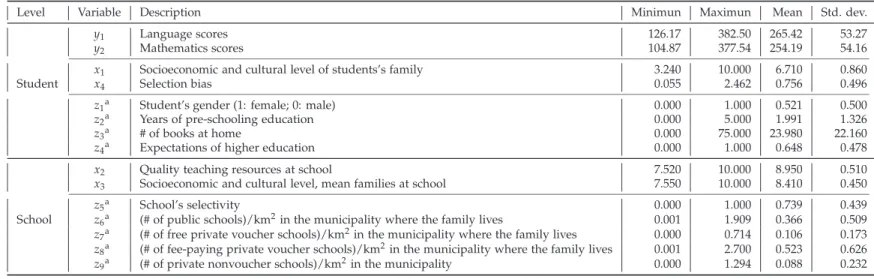
(15) (iii) free private voucher schools; and (iv) public schools. All of them are subject to the standardized testing system. For a detailed description of the Chilean school sector see, for instance, Anand et al. (2009), or Mizala and Romaguera (2004).3,4 Some basic information on the schools in our sample is reported in Table 1. Finally, the fifth database considered in this study comes from a larger study5 which carried out its own survey on the quality and quantity of resources, as well as the schools’ organizational skills. The questionnaires for this survey were responded by a minimum of five teachers from each school participating in the study.6 This survey allowed consideration of a variable usually unavailable in this type of studies which gathered information on the availability (quantity) and quality of teaching resources at each school. Merging the information contained in these five databases, to give a reasonable minimum number of students per school—and also to constrain the sample to schools that carry out standardized organizational procedures—we selected a sample comprising 176 schools within urban areas, each of which has more than 30 students who participated in the standardized tests, and had existed for more than three years prior to the study. Of these 176 schools, 7 were private nonvoucher schools, 69 were fee-charging private voucher schools, 11 were free private voucher schools, and 89 were public schools. It is also worth mentioning that out of the 7,826 schools carrying out the 4th year SIMCE basic education tests in 2008, only 2,742 met this criteria—i.e. urban schools operating for more than three years. Therefore, our sample does not entirely represent the universe of Chilean schools, which is composed of a large share of small and/or rural schools, although it is representative of the large urban schools which ultimately account for the largest share of students. In total, the sample consisted of 11,319 students from a variety of schools, socioeconomic levels, and regions across the country. Table 1 provides information on both the students and schools included in the sample. Consistent with both the information in the preceding paragraphs and the literature on school 3 In a previous version of the article, fee-charging private voucher schools and free private voucher schools were merged into one category—namely, privately owned subsidized schools. Following a referee’s advice, we finally decided to consider both categories separately, since private schools usually have more resources to spend in important areas which are not included in the teachers’ survey and, in addition, fee-charging private voucher schools might be especially selective in comparison to private nonvoucher schools, where owners can not only reject students based on expected performance, but also where families self-select based on their capacity or willingness to pay the fee. 4 In this respect, extensive literature compares that compares performance of public and private subsidized schools in Chile. Outstanding are the contributions by Gallego (2002, 2006) or Auguste and Valenzuela (2003), who investigated the effect of competition among schools on students’ achievement, finding that tighter competition contributes positively to increasing test scores. In contrast, McEwan and Carnoy (2000) and Hsieh and Urquiola (2006) found that private voucher schools skim off more advantaged families, relegating the most disadvantaged to the public schools. Another line of research, due to the availability of individual level data since 1997, considered the inclusion of controls for students’ resources, attempting to account for selection into different school sectors. Most of the studies following this line of research found that students attending voucher schools had only slightly better educational outcomes than those from public schools (see, for instance Mizala and Romaguera, 2001; Sapelli and Vial, 2002; Anand et al., 2009). A detailed review on the extant research on the Chilean voucher system is provided by Mizala and Torche (2012). 5 FONDECYT grant #11085061, Calidad y equidad en educación: Una estimación de dotaciones óptimas de recursos y capacidades en la educación básica de Chile utilizando modelos frontera (“Quality and equality in education: an estimation of optimal resource endowments and skills for the Chilean basic education system using frontier techniques”). 6 The study considered a representative sample of the universe of urban schools of basic education, comprising 288 schools (and 288 head teachers), and 1,485 teachers. Respondents to the questionnaires were mathematics and language teachers who taught classes to 4th year students of basic education taking the SIMCE examinations in 2008. A minimum of five surveys per school were performed in order to guarantee minimum reliability of results (Bass and Avolio, 1997).. 14.

(16) effectiveness using frontier techniques, our study considers data corresponding to the scores of fourthgrade students of basic education who took the SIMCE standardized tests in 2008. More specifically, the results corresponding to each student in the mathematics and language tests were obtained from the SIMCE database of student results (SIMCE, Resultados por alumno database) and were used as outputs (y1 and y2 , respectively). Regarding the selection of inputs, we considered the socioeconomic level of each student’s family as the first input (x1 ), which corresponds to a latent variable constructed through the use of confirmatory factor analysis. The variables included were: (i) father’s years of schooling, (ii) mother’s years of schooling, and (iii) family’s monthly income. The variables were obtained using the questionnaire answered by the parents of students participating in the SIMCE. At the school level, the variable “availability of quality teaching resources in the school” (x2 ) corresponds to a latent variable comprising five questions drawn from the questionnaire that had been answered by the teachers. Specifically, to construct this variable each teacher was asked to grade on a scale from 1 to 7, how appropriate the following resources (available at their respective schools) were to provide quality education: (i) teachers who taught on the initial courses of schooling (1st to 4th years); (ii) mathematics teachers; (iii) language teachers; (iv) science teachers; (v) other subject teachers. The variable was constructed using confirmatory factor analysis. When computing the latent variable score to quantify the latent variables used in this application, we obtained normalized results that contain both negative and positive values. Since nonparametric frontier models cannot handle negative values, the latent variable scores were transformed so that we had only positive values (Pastor, 1996). The variable “school’s average socioeconomic and cultural level” (x3 ) corresponds to the arithmetic mean of the variable “socioeconomic and cultural level of the student’s family.” As indicated in Section 2.1, we also consider a selection bias component in order to avoid confounding the relative effectiveness of schools with the background of their students. For this, as indicated earlier, we will consider a variant of the two-step corrections suggested by Heckman (1979), and we presume that a choice is made from four alternatives, namely, the four types of schools studied. Therefore, the following model is considered: ∗ Ic,d = Zc,d γd + νc,d ,. (11). ∗ is a latent variable, and Z where c is the student subindex, d is the school type (d = 1, 2, 3, 4), Ic,d c,d is a. vector of variables determining school choice. Since we are considering four types of schools, I will be a polychotomous variable taking values d = 1, 2, 3, 4—i.e. students have four choices. Assuming νc,d to be independently and identically distributed, following a type I extreme value distribution, we can estimate Equation (11) as a multinomial logit, whose estimates are then used to constructing a selection bias term for each observation, λc,d . In the common two-step correction proposed by Heckman (1979), this variable is analogous to the inverse Mills ratio, and therefore it can. 15.

(17) be expressed as: λc,d =. φ(Φ−1 ( Pc,d ) Pc,d. (12). where φ(·) is the standard normal density, Φ(·) is the normal distribution function, and Pc,d are the estimated probabilities yielded by the multinomial logit that student c chooses school type d (McEwan, 2001). In our particular application, the Zc,d values considering in the estimation of Equation (11), corresponding to the student level, are: (i) gender (1: female; 0: male); (ii) number of years of pre-schooling education; (iii) number of books in the student’s home; (iv) expectations of parents on the educational level achievable by their children (1: the expectations are to reach higher (university) education; 0: otherwise). Those corresponding to the school level are: (v) selectivity of the school, which is a dichotomous variable which takes the value of 1 when at least 50% of students’ parents were required to meet one of the following criteria when enrolling their children in the school: evaluation of the preschooling education, attendance at a games’ session, or passing an entrance examination; (vi) number of schools of each type per square kilometer in the student’s municipality. According to Goldhaber and Eide (2003), in order to be correctly identified, the choice model must contain at least one variable that is uncorrelated with the error term of the achievement model (Mizala and Torche, 2012). Although our model, based on the use of nonparametric frontiers, is much less affected by these issues, we consider it appropriate to stand with other papers dealing with similar issues—and, if possible, in the same context. Therefore, we follow a similar approach to that of Mizala and Torche (2012), which also uses the number of schools (of each type) per square kilometer in the students’ municipality, in order to control for the supply of schools of different sectors in the municipality where the family lives (a similar strategy is followed by McEwan, 2001, among others).7 According to these computations, these λcd would provide four λs for each student—one corresponding to each school type. From these four values, we will choose that corresponding to the school that student c is actually attending. This value is then included in the model as an additional input (x4 ). Table 2 reports summary statistics for the four selected variables at the student level (i.e. two outputs and two inputs), the two selected inputs at the school level, as well as the variables considered to construct the selection bias effect (some of them at student level, some at school level). We consider four models, each with different mixes of inputs and outputs. Specifically, model 1 has one input and two outputs, model 2 has two inputs and two outputs, model 3 has three inputs and two outputs, and model 4 has four inputs and two outputs, where x1 , x2 , x3 and x4 are the inputs and y1 and y2 are the outputs. 7 The results on the estimation of (11) are not provided for space reasons, given they would require the inclusion of several tables. However, they are available from the authors upon request.. 16.

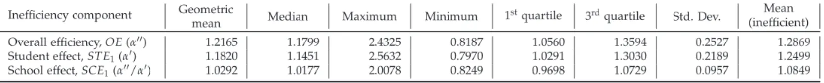
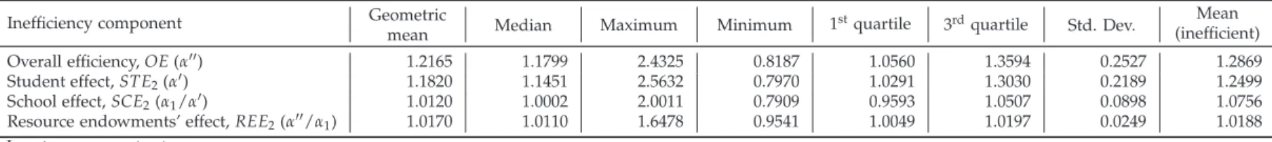
(18) 4.. Results. Table 3 reports order-m results for model 1 (bipartite decomposition of overall efficiency), which considers only student-level data. The first row in the table indicates that, on average (i.e., geometric mean), the overall inefficiency (α′′ ) obtained by maximizing outputs that corresponded to the 11,391 students from 176 schools in the sample was 1.2165; this is higher than the value of 1.1820 corresponding to the student effect in Equation (2) (although it corresponds to a lower efficiency level), which is presented in the second row of Table 3, α′ . As a result, the inefficiency attributable to the school (α′′ /α′ ) is 1.0292 (geometric mean). Therefore, on average, the contribution of the student effect to overall inefficiency is much higher than that attributable to the school. Table 3 provides some additional summary statistics (median, maximum, minimum, and standard deviation, along with first- and third-quartile values), in order to get some more insights on the distributions of overall efficiency and its components. Results corresponding to the tripartite decomposition of the overall efficiency included in model 2—which differs from model 1 on account of its inclusion of an additional effect at the school level (i.e., resource endowments effect)—are reported in Table 4. The presentation is analogous to that in Table 3 for model 1. In this case, the former school effect (SCE1 ) is decomposed into a more refined school effect (SCE2 ) and a resource endowment effect (REE2 ). The impact of the latter has a positive effect on overall inefficiency. However, on average, its magnitude (1.0170) is still much lower than that corresponding to the student effect, STE (1.1820), although slightly higher than the school effect. Results for the quadripartite decomposition of overall efficiency in model 3 are reported in Table 5 (summary statistics). In this model, an additional noncontrollable input, x3 , is included to control for the peer effect at the school level caused by the socioeconomic characteristics of its students—which we have collectively labeled as peer characteristics (a kind of contagion or emulation effect), PEE (McEwan, 2003). Compared to the tripartite decomposition (model 2), in this model it is the previous school-effect magnitude (SCE2 ) that is split into the peer effect (PEE3 ) and the net (residual) school effect (SCE3 ). With the overall efficiency and the student’s effect being constant, the inefficiency attributable to the school management is negligible, only −0.45% (α2 /α′ = 0.0045), as indicated in the third row of the table. The inefficiency of the peer effect PEE3 (i.e. 1.0165) is lower, on average, than the inefficiency due to the resource endowments (1.0170). Table 6 reports summary statistics of the results corresponding to the quinquepartite decomposition of overall efficiency in model 4. In this model, whose components are displayed on the right side of Figure 2, an additional input is included to control for the selection bias effect, SBE4 = (α2 /α3 ), which controls for unobserved attributes such as students’ motivation, ability, and ambition. The magnitude of this effect, on average (1.0093), is lower than that corresponding to both the peer effect and the resource endowment effect, and also lower than that corresponding to the student effect, but higher than that corresponding to the school effect (0.9863). However, this is an average (geometric mean) effect which conceals some relevant features of the distributions, as suggested by the values corresponding to the. 17.

(19) medians, which are closer (0.9773 for the school effect vs. 1.0025 for the selection bias effect). The movements showing the transition from model 1 (Table 3) to model 4 (Table 6) indicate that the student effect is always the most important component on the overall efficiency. The original magnitude corresponding to the school effect, SCE1 , is completely diluted in the peer (PEE4 ), resource endowments (REE4 ) and selection bias effects (SBE4 ). These results indicate that, on average, the nominal advantage of specific schools in terms of students’ performance are due to previous factors making the residual impact due to other possible factors almost negligible. In order to take into account more explicitly the fact that summary statistics might hide some relevant information, we considered some tools that allow for a fuller view of the distributions corresponding to the different components of the models considered. Specifically, using kernel methods, we made estimations of the densities corresponding to each indicator of model 4, i.e. of the quinquepartite decomposition of the overall effect. This information is reported in Figure 5, where the contributions of each component to the overall efficiency are added sequentially. The vertical lines correspond to the average of each effect. Figure 5.a displays the density corresponding to the student effect, STE, which exhibits a certain amount of bimodality in the vicinity of 1.15. The school effect corresponding to model 4, SCE4 , as indicated in Table 6, offsets the student effect, on average. Figure 5.b illustrates this fact, and we can see visually how the distributions corresponding to SCE4 and STE differ remarkably. Analogous to the bipartite decomposition analysis performed (model 1) in Figure 5.b, Figure 5.c illustrates how the inclusion of the resource endowment effect (REE) influences the relative contributions of each component of overall efficiency, while considering the full distributions of the effects. As shown in Figure 5.c, the impact of the resource endowments is much closer to the school effect, SCE4 , than to the student effect, STE, contributing modestly to overall efficiency. Estimates of densities are useful, because we can visually see how the SCE4 (dashed line) and REE (dotted line) differ. In the case of the resource endowments effect, the distribution is much tighter, pointing to a very homogeneous effect across schools. Analogous to both the bipartite and tripartite decompositions of overall efficiency, Figure 5.d displays the sequential densities corresponding to the relative contributions to overall efficiency when including the peer effects (PEE). The relative contribution of the entire distribution of the peer effect is very similar to that of the resource endowment effect (Figure 5.c). Indeed, Figures 5.c and 5.d are very difficult to distinguish, because the densities corresponding to REE and PEE overlap to a large degree. Finally, the contribution of the selection bias effect (SBE) considered by the quinquepartite decomposition to the overall school efficiency is included in Figure 5.e. Considering the scale of the figure, it is not easy to distinguish the selection bias effect from either the resource endowments or the peer effect. All of them have tight densities, indicating that the effect is homogeneous, whereas the flatter shape of the density corresponding to the school effect (SCE4 ) indicates a great deal of heterogeneity across schools.. 18.

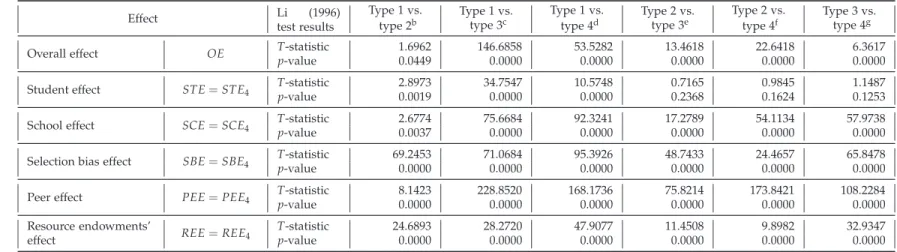
(20) Due to these discrepancies among the different densities, introduced sequentially, the emerging picture is of a much flatter distribution that corresponds to the overall efficiency effect, OE, as shown in Figure 5.f. This finding indicates that its components contribute in different ways, especially the school effect (SCE4 ), to the global effect, resulting in a bimodal distribution. This final distribution for overall efficiency (depicted with a thick solid line in Figure 5.f) is also much flatter than any of its components. In summary, according to these results, one may conclude that, regardless of the decomposition considered, overall inefficiency (α′′ ) is primarily caused by the student effect (α′ ), followed by the impact of the resource endowments (α′′ /α1 ), the peer effect (α1 /α2 ), the selection bias effect (α2 /α3 ) and only to a lesser degree by the net school effect (α3 /α′ ). Results differ remarkably among the different types of school listed in Table 7. On average, the overall inefficiency indicator (α′′ ) for public schools is the highest (1.2898), followed by free private voucher schools (1.2378). Private nonvoucher schools, meanwhile, are the most efficient (1.1028). However, these remarkable discrepancies are not attributable to school performance (α3 /α′ ), but to inefficiency at the student level (α′ ). Indeed, the student inefficiencies (α′ ) are, on average, 1.2139, 1.1786, 1.1523 and 1.1465 for public, free private voucher, fee-paying private voucher, and private nonvoucher schools, respectively. In addition, when analyzing the average inefficiency of inefficient schools, the (α3 /α′ ) parameter takes values of 1.0740, 1.0796, 1.0523 and 1.0661 for public, free private voucher, fee-paying private voucher, and private nonvoucher schools, respectively. However, although the mean inefficiencies of the two types of voucher schools do not differ notably, there are large discrepancies among them in terms of percentage of inefficient schools (63.64% vs. 37.68%). In the case of the private nonvoucher schools this percentage is much lower, 14.29%. Regarding the PEE and REE effects, their impact on public schools is virtually generalized, since most schools are inefficient for REE and PEE, respectively. However, as suggested, the differences referenced in the previous paragraphs are based on descriptive comparisons of averages for the different school types. Testing whether or not these differences for the means are statistically significant can be done using well-known instruments such as the Wilcoxon test. There have been some advances in the field of nonparametric statistics that allow performance of statistical tests, in order to compare whether entire distributions show significant differences—differences that are not restricted to a few moments within the distributions. These tests were introduced by Li (1996) and by several applications, such as those in Murillo-Melchor et al. (2010), Pastor and Tortosa-Ausina (2008), and Balaguer-Coll et al. (2010).8 Results are displayed in Table 8, which reports the results of testing the null hypothesis that the distributions of each of the variables are the same for pairs of types of schools compared. For instance, the T-statistic (which does not correspond to Student’s t), yielded by comparing the OE distributions of public vs. free private voucher schools, is 1.6962; this is significant at the 5% level. The differences between these types of schools are significant at this level for all effects. Actually, the differences are generally significant at the 1% significance level, with the exception of the student effect in the comparisons between private schools, 8 The. technical details of this test can be found in any of these articles, and also in Kumar and Russell (2002).. 19.

(21) regardless of their type, for which the differences are not significant at the usual levels (either at the 1%, 5% or even 10% significance level).. 5.. Conclusions. This paper contributes in two ways, one methodological and the other one empirical. The methodological contribution consists of evaluating educational performance considering a multilevel decomposition. Unlike previous studies that consider regression approaches in measuring student and school attainment, we consider frontier techniques which, in their nonparametric form, do not require the a priori specification of the functional form and which allow measurement the performance of each individual (i.e., a student) in terms of best-practice performance. Likewise, some recent but scarce contributions— such as De Witte et al. (2010)—consider order-m techniques so that both the curse of dimensionality and the influence of outliers are largely alleviated, resulting in statistically robust results. In contrast to the proposal of De Witte et al. (2010) and those of Silva Portela and Thanassoulis (2001); Thanassoulis and Silva Portela (2002), who only consider student-level variables, the models in this paper consider school-level variables as well. Both the literature pertaining to multilevel models in education (see, for instance, Cervini, 2009; Blanco, 2010) and the results obtained in the application carried out in this paper suggest that it is convenient and necessary to include these types of variables for three main reasons. First, if school-level variables were not considered, we would undervalue the performance of those schools that either enroll students with unfavorable socioeconomic situations or that have suboptimal resource endowments. Indeed, results show large global and school inefficiencies that are attributable not to the management of the school, but rather to the effect of students’ emulation of other students (the so-called peer effect) and with policy that results in inadequate resource endowments (the so-called resource endowments effect). Second, our analysis by type of school (i.e. public, free private voucher, fee-paying private voucher, and private nonvoucher) indicates that the large discrepancies among the different types diminish sharply when school-level variables are included in the analysis. Third, they allow for the inclusion of relevant extra information in examinations of the analyzed phenomenon. From an empirical point of view, results show that the large discrepancies found among schools in model 1 (which considers only the student effect and the school effect) fade away when the schoollevel variables are introduced sequentially. However, and in spite of controlling for peer, resource endowments, and selection bias effects, public schools’ performance is lower than that of fee-paying private voucher and private nonvoucher schools, and the discrepancies are statistically significant. This result does not hold when comparing with free private voucher schools, whose performance is statistically lower than that of public schools. Indeed, in comparing public schools and free private voucher schools—both of which compete for similar students—it becomes clear that the global efficiency estimator for public schools is, on average, 1.2898, higher than that of free private voucher schools, whose. 20.

(22) average is 1.2378. However, these differences are not caused by management differences between school type (1.0015 vs. 1.0129 for public and free private voucher schools, respectively), but rather to remaining factors, especially those related to student characteristics. Indeed, the average negative effect of REE is, in public schools, more than twice that of free private voucher schools, and the peer effect attributable to student characteristics is also considerably higher in public schools than in fee-paying private voucher schools and private nonvoucher schools. These results reinforce both those views advocating a separate analysis of the two types of voucher schools, as well as those others considering that the fees raised by fee-paying private voucher schools enable the acquisition of important resources for the school (beyond the teaching resources), contributing to the persistence of the differences between public and private education. One may expect that the inclusion of other variables that proxy for resources would contribute to a further reduction in this gap. This result is in line with that of Thieme et al. (2011), who indicate that, in Chile, the potential gains of school achievement due to higher resource endowments surpass those one might obtain due to a better school management. The results of the current study roughly coincide with those of other studies in the field of education research, most of which find that fewer than 30% of variance in the results of students’ educational achievement are due to the school effect. Indeed, the 6.68% that we obtained as the average level of inefficiency among inefficient schools, for example, is very close to the 6.80% found by Mizala et al. (2002). From the public management point of view, the main implication of this research is that the technological gap separating conditional frontiers from the overall metafrontier can be reduced, but this requires the implementation of specific decisions in order to reduce these inefficiencies. According to the results obtained, it appears that the most important source of school inefficiency is the resource endowment effect, followed closely by the peer effect. This result is particulary relevant, since it affects especially both public and free private voucher schools, which cannot obtain fees from families, and whose students come generally from the most vulnerable communities in Chile. This result is in line with previous results such as those by Valenzuela et al. (2009), who found that the voucher system has a remarkable effect on the high socioeconomic segregation of the Chilean educational system, or Hsieh and Urquiola (2006), who considered that this segregation can be exacerbated by the competitive mechanisms to attract students.. 21.