TítuloExperimental validation of a multibody model for a vehicle prototype and its application to automotive state observers

Texto completo

(1)Departamento de Ingenierı́a Industrial II Escuela Politécnica Superior University of La Coruña. Experimental Validation of a Multibody Model for a Vehicle Prototype and its Application to Automotive State Observers. Roland Pastorino. A thesis submitted for the degree of. Doctor Ingeniero Industrial. Advisor: Miguel Ángel Naya Villaverde Co-advisor: Javier Cuadrado Aranda. Ferrol, June 2012.

(2)

(3) A ma famille pour son soutien inconditionnel depuis toujours..

(4)

(5) Resumen. Introducción La dinámica de vehı́culos ha sido un campo de aplicación de la mecánica desde hace varias décadas. Antes de la llegada de los ordenadores personales en los años setenta, la dinámica de vehı́culos se estudiaba de forma analı́tica debido a las limitaciones de las matemáticas para resolver grandes sistemas. Hasta el momento, los modelos de vehı́culo eran relativamente simples ya que tenı́an que ser formulados de manera analı́tica. Con la aparición de los ordenadores comenzó a desarrollarse la disciplina relacionada con la simulación de sistemas multicuerpo. Esta disciplina está basada en métodos computacionales como la integración numérica para el cálculo de la dinámica de sistemas mecánicos complejos. Desde entonces las caracterı́sticas de los ordenadores y las simulaciones multicuerpo han mejorado sustancialmente. Los modelos multicuerpo de vehı́culo y los programas de simulación destinados al análisis de la dinámica de vehı́culos pronto han aparecido en los años ochenta para compensar la falta de modelos completos de vehı́culos (Körtum, 1985). Estos modelos han ganado en complejidad y precisión para incluir algunos comportamientos y caracterı́sticas de los componentes del vehı́culo y de sus subsistemas que no se consideraban anteriormente. Como consecuencia de esta evolución, el campo de la dinámica de vehı́culos se ha dividido en subcampos de aplicaciones como por ejemplo las simulaciones de vehı́culos para su ejecución en tiempo real, el análisis del comportamiento o del confort. El Laboratorio de Ingenierı́a Mecánica de la Universidad de La Coruña se ha especializado en la simulación de modelos multicuerpo en tiempo real (Cuadrado et al., 2000, 2004a,b). La dinámica de vehı́culos en tiempo real es uno de sus campos de aplicación. Las coordenadas naturales y una formulación multicuerpo desarrollada en el Laboratorio, que permite simular mecanismos complejos en tiempo real con precisión y robustez, son las elecciones preferidas para modelizar vehı́culos en el Laboratorio (Naya et al., 2007). Esta tesis pretende aportar nuevos elementos para un mejor entendimiento de esta lı́nea de investigación. En la práctica, la fiabilidad y la validez, que representan caracterı́sticas de gran importancia a la hora de desarrollar modelos de vehı́culo, deben ser investigadas para los métodos de modelización de vehı́culos desarrollados en el Laboratorio. En efecto, es primordial verificar que la implementación sea correcta y también ajustar el grado de precisión del modelo a los requerimientos de la aplicación. A. H. Hoskins ha expresado claramente la necesidad de la validación afirmando que “Sin validación de la dinámica del vehı́culo solamente existe especulación que un modelo determinado prediga con precisión la respuesta del vehı́culo” (Hoskins and El-Gindy, 2006). Cualquier validación implica realizar ensayos experimentales para recabar datos de referencia que se comparan con los resultados de las simulaciones. La metodologı́a de realización de los ensayos debe permitir generar los mejores datos de referencia posibles. Una de las únicas y la más completa metodologı́a de validación de modelos de vehı́culos es la que se ha desarrollado para validar el National Advanced Driving Simulator (Garrott et al., 1997). Por consiguiente, se ha empleado en esta investigación. Hoy en dı́a, varios modelos simplificados de vehı́culo se emplean comúnmente en contro-.

(6) ladores de estabilidad embarcados (Tseng et al., 1999). El siguiente paso en la evolución de estos controladores serı́a el uso de modelos multicuerpo que se ejecutan en tiempo real. Esta evolución es comparable a la pasada evolución de las simulaciones de la dinámica de vehı́culos de modelos clásicos de vehı́culo a modelos multicuerpo. El uso de modelos multicuerpo de vehı́culo que se ejecutan en tiempo real en observadores de estados es un tema de investigación recientemente iniciado en el Laboratorio de Ingenierı́a Mecánica (Cuadrado et al., 2010, 2011). El empleo de técnicas de estimación de estados y modelos de vehı́culos altamente detallados deberı́a proporcionar información no disponible si se usan modelos clásicos de vehı́culos. La substitución de los modelos clásicos por modelos multicuerpo no es trivial. Se deben investigar las diferentes maneras de escribir las ecuaciones del movimiento que aparecen en las varias formulaciones multicuerpo para que puedan ser empleadas con la máxima eficiencia posible en los observadores más comunes para sistemas nolineales (Grewal and Andrews, 2008). También cabe investigar los observadores para sistemas nolineales más recientes y ver si se adaptan mejor cuando se emplean con modelos multicuerpo (Julier and Uhlmann, 2004).. Metodologı́a Una precisa metodologı́a ha sido empleada a lo largo de todo este trabajo. Para cada parte de éste, un estudio exhaustivo de los mejores artı́culos cientı́ficos, libros sobre la materia, grupos nacionales e internacionales de investigación ha sido llevado a cabo con el objetivo de conocer las prácticas actuales ası́ como las lı́neas de investigación de otros grupos. La información recabada ha servido para valorar y guiar la investigación durante el transcurso de esta tesis. Periódicamente y desde el principio de esta investigación, los avances más significativos de ésta se han recopilado y presentados en los principales congresos nacionales e internacionales del campo correspondiente, con el fin de comprobar la calidad y la pertinencia del trabajo ası́ como de constatar el interés suscitado. Fruto de estos valiosos comentarios crı́ticos, algunos de estos trabajos se han mejorado y ampliado para ser publicados en las revistas cientı́ficas más prestigiosas de cada campo abarcado por este trabajo. Una lista de todos los artı́culos que se han publicado o que han sido aceptados y están a punto de ser presentados o publicados se encuentra a continuación. Según esta metodologı́a, los últimos artı́culos en haber sido presentados en congresos se mejorarán y ampliarán para ser enviados a revistas cientı́ficas después o durante los últimos meses de esta tesis. Por otra parte, como lo indica el tı́tulo de esta tesis, uno de sus objetivos de esta investigación es la validación de un modelo multicuerpo de un prototipo de vehı́culo. Con el fin de obtener los mejores datos experimentales para validar este modelo, la completa y reconocida metodologı́a de validación del National Advanced Driving Simulator ha sido aplicada. Comparaciones entre estos datos experimentales y los resultados de las simulaciones son la clave para demostrar la validez y la precisión del modelo multicuerpo desarrollado.. Conclusiones Este trabajo se ha centrado en la investigación sobre modelos multicuerpo de vehı́culos para su ejecución en tiempo real y su aplicación a observadores de estados. Su aportación principal ha sido la elaboración de directrices para el desarrollo de dichos modelos y para la investigación teórica y práctica sobre su uso en observadores de estados Primero, para evaluar la validez de las predicciones de las simulaciones, parte de la completa.

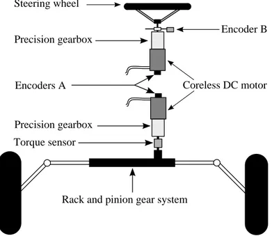
(7) metodologı́a desarrollada para validar el modelo multicuerpo de vehı́culo del National Advanced Driving Simulator ha sido aplicada. Un prototipo de vehı́culo automatizado ha sido construido con el objetivo de repetir maniobras de referencia y generar datos de referencia para la validación. Durante el desarrollo de este prototipo, se ha hecho especial hincapié en el sistema de retorno de fuerzas al conductor que forma parte del sistema de dirección por cables (steer–by–wire). Un enfoque general para modelizar con precisión el conjunto amplificador– motor–reductora ha sido desarrollado y validado empleando el sistema de retorno de par al conductor de bajo coste compuesto por una reductora con planetarios de dos etapas, un motor de corriente continua con imanes permanentes y sin núcleo, y finalmente un amplificador lineal de cuatro cuadrantes. Este enfoque, que tiene en cuenta los juegos, la flexibilidad, el rozamiento estático y dinámico, ası́ como los procedimientos de identificación, es aplicable a una gama amplia de conjuntos amplificador–motor–reductora. Una vez que el prototipo de vehı́culo se ha automatizado completamente, dos maniobras a bajas velocidades implicando la dinámica longitudinal del vehı́culo y también la lateral han sido repetidas 7 veces en una zona del campus de la escuela de Ingenierı́a. Los datos experimentales de referencia han sido obtenidos de las dos maniobras con el objetivo de validar el modelo de vehı́culo. Después, la segunda parte de esta tesis ha sido dedicada al desarrollo de un modelo matemático del prototipo de vehı́culo automatizado mencionado anteriormente. Se trata de un modelo multicuerpo, con 14 grados de libertad, que se ejecuta en tiempo real y que ha sido preparado utilizando una librerı́a para modelos multicuerpo en lenguaje FORTRAN ası́ como un entorno de simulación programado en C++ que incluye un entorno gráfico fiel a la realidad, un perfil preciso de la pista de prueba y detección de colisiones. El perfil preciso de la pista de pruebas ha sido obtenido mediante un levantamiento topográfico. Los subsistemas como los neumáticos o los frenos también han sido modelizados. Con el fin de comprobar la validez del modelo, los datos experimentales de referencia obtenidos de los sensores del vehı́culo han sido usados como entradas para el modelo para repetir las dos maniobras de referencia en el entorno de simulación. Entonces, determinadas variables de simulación han sido comparadas a sus homólogas experimentales provistas de un intervalo de confianza que caracteriza los errores del proceso de prueba en pista. Se han interpretado los resultados de las comparaciones para extraer directrices prácticas a la hora de preparar modelos de vehı́culo que se ejecutan en tiempo real. Finalmente, el uso de modelos multicuerpo para simulaciones en tiempo real con observadores de estados ha sido investigado. El primer observador considerado ha sido el filtro de Kalman extendido en forma continua. Se ha investigado el empleo de dos formulaciones multicuerpo (la formulación matriz–R y la formulación por penalizadores) usando un mecanismo de 4 barras. El método de matriz–R, que ha demostrado tener mejor comportamiento y eficiencia que la formulación por penalizadores, se ha aplicado a un modelo multicuerpo complejo: el modelo de un Volkswagen Passat. A pesar de la precisión del filtro, no fue posible simular el modelo en tiempo real. Por consiguiente, nuevos desarrollos teóricos e implementaciones prácticas utilizando otro tipo de observadores nolineales, los filtros de Kalman de tipo sigma–point, han sido llevados a cabo con un mecanismo de 5 barras. Como resultado de la aplicación de estos observadores, se ha demostrado que el uso de integradores implı́citos apenas aporta mejora comparado con el uso de sus homólogos explı́citos, llevando de esta manera a una menor carga computacional para todos los filtros mencionados. Los filtros de Kalman de tipo sigma–point han demostrado tener mejor precisión pero una carga computacional más elevada que el filtro.

(8) de Kalman extendido en su forma continua. Sin embargo, presentan varias ventajas sobre este último: una implementación más sencilla, una estructura fácilmente paralelizable que ayuda a alcanzar el tiempo real y el posible uso de cualquier formulación multicuerpo que también ayude a reducir el coste computacional. A la vista de estos resultados, la elección del conjunto observador, formulación multicuerpo e integrator depende de los requisitos de la aplicación y es un compromiso entre la precisión de la estimación y la eficiencia computacional.. Lista de publicaciones cientı́ficas Un total de once artı́culos han sido publicados en diversas revistas cientı́ficas de prestigio y congresos internacionales y nacionales. Un último artı́culo será presentado en el mes de noviembre en el Congreso Nacional de Ingenierı́a Mecánica. Artı́culos de revistas cientı́ficas Cuadrado J. , Dopico D. , Pérez J. A. , and Pastorino R. . Automotive observers based on multibody models and the Extended Kalman Filter. Multibody System Dynamics, 27(1): 3–19, 2011. doi: 10.1007/s11044-011-9251-1. iv, 4, 105, 112 Pastorino R. , Naya M. A. , Pérez J. A . , and Cuadrado J. . Geared PM coreless motor modelling for driver’s force feedback in steer–by–wire systems. Mechatronics, 21(6):1043– 1054, 2011. doi: 10.1016/j.mechatronics.2011.05.006. 20. Artı́culos de congresos internacionales y nacionales Cuadrado J. , Dopico D. , Pérez J. A. , and Pastorino R. . Influence of the sensored magnitude in the performance of observers based on multibody models and the extended Kalman filter. In Proceedings of the Multibody Dynamics ECCOMAS Thematic Conference, Warsaw, Poland, June 2009. 4, 100, 111 Cuadrado J. , Dopico D. , Naya M. A. , and Pastorino R. . Automotive observers based on multibody models and the extended Kalman filter. In The 1st Joint International Conference on Multibody System Dynamics, Lappeenranta, Finland, May 2010. iv, 4, 105, 112 Pastorino R. . La simulation des systèmes multicorps dans l’automobile. Interface, revue des ingénieurs des INSA de Lyon, Rennes, Rouen, Toulouse, (111):22, 3ème et 4ème trimestre 2011. Pastorino R. , Naya M. A. , Pérez J. A. , and Cuadrado J. . X–by–wire vehicle prototype: a steer– by–wire system with geared PM coreless motors. In Proceedings of the 7th EUROMECH Solid Mechanics Conference, Lisbon, Portugal, September 2009. 10 Pastorino R. , Naya M. A. , Luaces A. , and Cuadrado J. . X–by–wire vehicle prototype: automatic driving maneuver implementation for real–time MBS model validation. In Proceedings of the 515th EUROMECH Colloquium, Blagoevgrad, Bulgaria, 2010. 10, 14.

(9) Pastorino R. , Dopico D. , Sanjurjo E. , and Naya M. A. . Validation of a multibody model for an x–by–wire vehicle prototype through field testing. In Proceedings of the ECCOMAS Thematic Conference Multibody Dynamics 2011, Brussels, Belgium, 2011a. Pastorino R. , Naya M. A. , Luaces A. , and Cuadrado J. . X–by–wire vehicle prototype : a tool for research on real–time vehicle multibody models. In Proceedings of the 13th EAEC European Automotive Congress, Valencia, Spain, June 2011b. Pastorino R. , Richiedei D. , Cuadrado J. , and Trevisani A. . State estimation using multibody models and unscented Kalman filters. In Proceedings of the 524th EUROMECH Colloquium, Enschede, Netherlands, 2012a. Pastorino R. , Richiedei D. , Cuadrado J. , and Trevisani A. . State estimation using multibody models and nonlinear Kalman filters. In The 2nd Joint International Conference on Multibody Systems Dynamics, Stuttgart, Germany, May 2012b. Sanjurjo E. , Pastorino R. , Dopico D. , and Naya M. A. . Validación experimental de un modelo multicuerpo de un prototipo de vehı́culo automatizado. In XIX Congreso Nacional de Ingenierı́a Mecánica (to be presented), Castellón, Spain, Nov. 2012..

(10)

(11) Abstract. The simulation of multibody system dynamics is a key element of Computer–Aided Design and also a well–established tool in the development of new vehicles. A vehicle model is a typical multibody system made of rigid and/or flexible bodies that are interconnected by joints and usually undergo large translational and rotational displacements. In the last decade, real–time simulations of vehicle multibody models have gained interest thanks to the development hardware– or human–in–the–loop applications. Efficient multibody formulations must be employed to simulate complex systems in real–time and reliability of the models and validity are of the highest importance. This thesis focuses first on the study of the validity of real–time vehicle multibody models developed at the Laboratorio de Ingenierı́a Mecánica of the University of La Coruña. For this purpose, a vehicle prototype has been built and automated in order to repeat reference maneuvers. The numerous sensors on the prototype gather the most relevant magnitudes of the vehicle motion (roll–pitch–yaw rates, wheel speeds, etc). Two low speed maneuvers involving the longitudinal and lateral vehicle dynamics have been repeated several times in a test area at the campus of the engineering school. A real–time multibody model of the vehicle prototype has been prepared as well as a simulation environment that includes a close graphical environment, a true road profile and collision detection. Subsystems like brakes or tires have also been modeled. Both test maneuvers have been repeated with the developed multibody model in the simulation environment using inputs that have been measured experimentally. Selected simulation variables have then been compared to their experimental counterparts provided with a confidence interval that characterizes the field testing process errors. The results of the comparisons have then been interpreted to extract useful guidelines to build real–time vehicle multibody models. Once a real–time vehicle model is validated, it not only raises the possibility to be used in hardware– or human–in–the–loop applications but also in on–board stability controllers. Nowadays simplified vehicle models coming from the classical vehicle dynamics theory are commonly employed in on–board stability controllers. The use of real–time vehicle multibody models in state observers (a widely–used control technique in stability controllers) is a research subject initiated a few years before the beginning of this thesis at the Laboratorio de Ingenierı́a Mecánica. The last part of this thesis goes first over the developed implementation of the Extended Kalman filter, a common state observer for nonlinear systems, with multibody models and, after that presents several new implementations using this filter and other filters coming from the family of the sigma–point Kalman filters..

(12)

(13) Résumé. La simulation de la dynamique des systèmes multicorps est un élément clef de la conception assistée par ordinateur (CAO) et aussi un outil bien établi dans le développement de nouveaux véhicules. Un modèle de véhicule est un système multicorps typique composé de corps rigides et/ou flexibles qui sont interconnectés par des liaisons mécaniques et qui généralement subissent de grands déplacements autant en translation qu’en rotation. Au cours de la dernière décennie, les simulations de modèles multicorps de véhicules en temps réel ont suscité un grand intérêt grâce au développement de simulations hybrides interactives. Des formulations multicorps efficaces doivent être employées pour simuler des systèmes complexes en temps réel et la fiabilité et la validité de ces modèles sont d’importance vitale. Cette thèse se concentre d’abord sur l’étude de la validité des modèles multicorps de véhicule qui se développent pour des applications en temps réel au Laboratorio de Ingenierı́a Mecánica de l’Université de La Corogne. Pour ce faire, un prototype de véhicule a été fabriqué et automatisé dans le but de répéter des manœuvres de référence. De nombreux capteurs montés dans le prototype recueillent les magnitudes les plus pertinentes du mouvement du véhicule (roulis–tangage–lacet, vitesses des roues, etc). Deux manœuvres à basse vitesse qui impliquent la dynamique longitudinale et latérale du véhicule ont été répétées plusieurs fois dans une zone du campus de l’école d’ingénieurs. Un modèle multicorps temps réel du prototype de véhicule a été préparé ainsi qu’un environnement de simulation qui inclut un environnement graphique réel, un profil réaliste de la piste d’essai et détection de collisions. Les sous–systèmes comme les freins ou les pneumatiques ont aussi été modélisés. Les deux manœuvres d’essai ont été répétées avec le modèle multicorps dans l’environnement de simulation en utilisant des entrées mesurées expérimentalement. Certaines variables de simulation ont été ensuite comparées avec leurs homologues expérimentales pourvues d’un intervalle de confiance qui caractérise les erreurs du procédé d’essai sur piste. Les résultats de la comparaison sont alors interprétés pour soustraire des règles utiles dans le développement de modèles multicorps temps réel de véhicules. Une fois qu’un modèle multicorps a été validé, il n’est pas seulement envisageable de l’utiliser pour des simulations hybrides ou interactives mais aussi pour des contrôleurs de stabilité embarqués. Dans l’actualité, des modèles de véhicule simplifiés provenant de la théorie classique de la dynamique du véhicule s’utilisent communément dans des contrôleurs de stabilité embarqués. L’utilisation de modèles multicorps temps réel de véhicule dans des observateurs d’état (une technique de contrôle très connue pour les contrôleurs de stabilité) est un sujet de recherche initié quelques années avant le début de cette thèse au Laboratorio de Ingenierı́a Mecánica. La dernière partie de cette thèse examine d’abord en détail l’implémentation développée jusqu’à présent utilisant filtre de Kalman étendu, un observateur d’état habituel pour les systèmes nonlinéaires et modèles multicorps. Ensuite de nouvelles implémentations utilisant ce même filtre ainsi que d’autres filtres provenant de la famille des filtres de Kalman de type sigma–point sont présentées ..

(14)

(15) Resumo. A simulación da dinámica de sistemas multicorpo é un elemento clave do deseño asistido por ordenador. É tamén unha ferramenta ben establecida no desenvolvemento dos novos vehı́culos. Un modelo de vehı́culo é un sistema multicorpo tı́pico composto por corpos rı́xidos e/o flexibles interconectados por unións. Xeralmente, estos corpos experimentan grandes desplazamentos tanto na traslación como na rotación. Nesta derradeira década, simulacións de modelos multicorpo de vehı́culo en tempo real suscitou especial interese. Este tipo de simulacións vai destinado a aplicacións hardware– o human–in–the–loop. Deben ser empregadas formulacións multicorpo eficientes para simular sistemas complexos en tempo real. A fiabilidade e a validez destes modelos son de vital importancia. Esta tese céntrase no estudio da validez dos modelos multicorpo que desenvólvense para aplicacións en tempo real no Laboratorio de Enxeñerı́a Mecánica da Universidade da Coruña. Con este fin, un prototipo de vehı́culo fabricouse e automatizouse co obxectivo de repetir manobras de referencias. Numerosos sensores recollen as magnitudes máis relevantes do movemento do vehı́culo (balanceo–cabeceo–guiñada, velocidades das rodas, etc). Dos manobras a baixas velocidades que involucrán a dinámica lonxitudinal e lateral do vehı́culo foron repetidas varias veces nunha zoa do campus da escola de enxe?erı́a. Preparouse un modelo multicorpo do prototipo do vehı́culo para unha execución en tempo real e un entorno de simulación que integra un entorno gráfico real, o verdadeiro perfil da pista e unha detección de colisións. Tamén foron modelados subsistemas como os freos e os neumáticos. Ambas manobras de proba foron medidas experimentalmente. A continuación, determinadas variables de simulación foron comparadas coas súas homólogas experimentais provistas dun intervalo de confianza que caracteriza os errores do proceso de ensaio na pista. Entón, o resultados da comparación foron interpretados para extraer pautas útiles para desenvolver modelos multicorpo de véhiculos que execútanse en tempo real. Unha vez que o modelo multicorpo do vehı́culo é validado, no soamente surxe a posibilidade de usarlo en aplicacións hardware– y/o human–in–the–loop mais tamén en controladores de estabilidade embarcados. Na actualidade, modelos de vehı́culos simplificados provintes da teorı́a clásica da dinámica de vehı́culos empréganse comúnmente en controladores de estabilidade embarcados. O uso de modelos multicorpo de vehı́culos capaces de executarse en tempo real en observadores de estados (unha técnica de control ampliamente coñecida en controladores de estabilidade) é un tema de investigación iniciado poucos anos antes do inicio desta tese no Laboratorio de Enxeñerı́a Mecánica. A derradeira parte desta tese trata primeiro a implementación desenvolta ata agora co filtro de Kalman estendido en modelos multicorpo. Despois preséntanse novas implementacións empregando este mismo filtro ası́ como outros pertencentes a familia dos filtros de Kalman tipo sigma–point..

(16)

(17) Acknowledgements. It is an undeniable fact that a thesis is first and foremost a personal achievement. However the integration into a research group is one of the keys of any thesis. Among all the researchers that surrounded me since my arrival to the Laboratorio de Ingenierı́a Mecánica (LIM) at the end of 2007, I wish first to warmly thank my advisors, Miguel and Javier, whose invaluable support has been a factor of success. I would also like to express my gratitude to the LIM research team: Alberto, Daniel, Urbano, Fran, Manuel, Amelia, Emilio and Jairo, who with their advice showed me the way in the darkest parts of my thesis. Special thanks go to Dario Richiedei and Alberto Trevisani, as well as the whole research team of the Mechatronics laboratory of Vicenza, for the fruitful collaboration. Usually, research laboratories mainly rely on public funds, so I would like to thank the Spanish Ministry of Science and Innovation and ERDF funds through the grant TRA2009-09314 too for its support in this research. During a thesis, the working-day does not end when you close the door of the laboratory late in the evening. For this reason, I wholeheartedly want to thank my parents (Denise and Jean-Yves) and my brothers (Nicolas and David) for their unconditional support, as well as to apologize for my too short and sporadic stays at home. Last but not least, I want to thank Carolina for encouraging me despite having bravely endured countless and incomprehensible scientific lucubrations..

(18)

(19) Agradecimientos. Es un hecho indiscutible que una tesis es ante todo un logro personal. Sin embargo la integración en un grupo de investigación constituye una de las claves de cualquier tesis. Entre todos los investigadores que me rodearon desde mi llegada al Laboratorio de Ingenierı́a Mecánica (LIM) a finales de 2007, quisiera primero dar las gracias a mis directores, Miguel y Javier, cuyo apoyo inestimable ha sido un factor de éxito. Me gustarı́a también expresar mi gratitud al grupo de investigación del LIM : Alberto, Daniel, Urbano, Fran, Manuel, Amelia, Emilio y Jairo, quienes con sus consejos me orientaron en las partes más oscuras de mi tesis. Dirijo unos agradecimientos especiales a Dario Richiedei y Alberto Trevisani, ası́ como a todo el grupo de investigación del Laboratorio de Mecatrónica de Vicenza, por la fructı́fera colaboración. Generalmente, los laboratorios de investigación dependen principalmente de fondos públicos, por lo que quisiera agradecer el apoyo del Ministerio de Ciencia e Innovación ası́ como de los fondos ERDF a través de la subvención TRA2009-09314. Durante una tesis, la jornada laboral no se termina al cerrar la puerta del laboratorio tarde por la noche. Por esta razón, quiero de todo corazón dar las gracias a mis padres (Denise y Jean-Yves) y a mis hermanos (Nicolas y David) por su apoyo incondicional, ası́ como disculparme por mis estancias en casa demasiado cortas y esporádicas. Por último, si bien no menos importante, quisiera dar las gracias a Carolina por haberme animado a pesar de haber soportado innumerables e incomprensibles elucubraciones cientı́ficas..

(20)

(21) Remerciements. Il est irréfutable qu’une thèse est avant tout une réussite personnelle. Cependant l’intégration dans un groupe de recherche est une des clefs de n’importe quelle thèse. Parmi tous les chercheurs que j’ai côtoyés depuis mon arrivée au Laboratorio de Ingenierı́a Mecánica (LIM) à la fin de l’année 2007, je voudrais d’abord chaleureusement remercier mes directeurs, Miguel et Javier, dont le soutien inestimable a été un facteur de réussite. Je souhaiterais exprimer également ma reconnaissance à toute l’équipe de recherche du LIM : Alberto, Daniel, Urbano, Fran, Manuel, Amelia, Emilio et Jairo, qui avec leurs conseils m’ont montré le chemin dans les parties les plus obscures de ma thèse. Des remerciements spéciaux vont à Dario Richiedei et Alberto Trevisani, ainsi qu’à tout le groupe de recherche du Laboratoire de Mécatronique de Vicence, pour la collaboration fructueuse. Généralement, les laboratoires de recherche dépendent principalement de fonds publiques pour ce que je voudrais remercier le soutien du Ministère des Sciences et de l’Innovation espagnol ainsi que les fonds ERDF à travers de la subvention TRA2009-09314. Au cours d’une thèse, la journée de travail ne se termine pas lorsque l’on ferme la porte du laboratoire tard le soir. Pour cette raison, je veux de tout cœur remercier mes parents (Denise et Jean-Yves) et mes frères (Nicolas et David) pour leur soutien inconditionnel, et aussi leurs présenter mes excuses pour mes séjours à la maison trop courts et sporadiques. Mon dernier remerciement, et non des moindres, va à Carolina pour m’avoir encouragé en dépit d’avoir enduré d’innombrables et incompréhensibles élucubrations scientifiques..

(22)

(23) Contents List of Figures. xxiii. List of Tables. xxvii. List of Datasheets. xxix. Acronyms. xxxi. Glossary. xxxv. 1 Introduction 1.1 Motivations . . . . . . . . . . . . . . . . . . 1.2 State of the art of multibody analysis in the 1.3 Objectives . . . . . . . . . . . . . . . . . . . 1.4 Thesis structure . . . . . . . . . . . . . . . .. . . . .. . . . .. . . . .. . . . .. . . . .. . . . .. . . . .. 1 2 2 4 5. 2 Field testing using an X–by–wire vehicle prototype 2.1 The validation methodology . . . . . . . . . . . . . . . . . . . . . . 2.1.1 Background and state of the art of vehicle model validation 2.1.2 The validation methodology developed for the NADS . . . 2.2 The X–by–wire vehicle prototype . . . . . . . . . . . . . . . . . . . 2.2.1 Overview . . . . . . . . . . . . . . . . . . . . . . . . . . . . 2.2.2 The digital acquisition system . . . . . . . . . . . . . . . . . 2.2.3 By-wire systems . . . . . . . . . . . . . . . . . . . . . . . . 2.2.4 Extra sensors . . . . . . . . . . . . . . . . . . . . . . . . . . 2.3 Driver’s force feedback of the steer–by–wire . . . . . . . . . . . . . 2.3.1 System description . . . . . . . . . . . . . . . . . . . . . . . 2.3.2 Model equations . . . . . . . . . . . . . . . . . . . . . . . . 2.3.3 Identification procedures and simulation results . . . . . . . 2.3.4 Discussion . . . . . . . . . . . . . . . . . . . . . . . . . . . . 2.4 Test maneuvers . . . . . . . . . . . . . . . . . . . . . . . . . . . . . 2.4.1 Sensor data post-processing . . . . . . . . . . . . . . . . . . 2.4.2 Low speed straight–line maneuver . . . . . . . . . . . . . . 2.4.3 Low speed J–turn maneuver . . . . . . . . . . . . . . . . . .. . . . . . . . . . . . . . . . . .. . . . . . . . . . . . . . . . . .. . . . . . . . . . . . . . . . . .. . . . . . . . . . . . . . . . . .. . . . . . . . . . . . . . . . . .. . . . . . . . . . . . . . . . . .. 7 8 8 9 10 10 12 14 17 19 20 22 29 38 39 40 40 41. 3 Vehicle modeling and simulation environment 3.1 Vehicle modeling . . . . . . . . . . . . . . . . . . . . . . . . . . . . . . . . . . 3.1.1 Multibody formulation and integrator . . . . . . . . . . . . . . . . . .. 47 48 48. xxi. . . . . . . . . . . automotive field . . . . . . . . . . . . . . . . . . . .. . . . .. . . . ..

(24) Contents. . . . . . .. . . . . . .. . . . . . .. . . . . . .. . . . . . .. . . . . . .. . . . . . .. . . . . . .. . . . . . .. . . . . . .. . . . . . .. . . . . . .. . . . . . .. . . . . . .. . . . . . .. . . . . . .. 50 73 80 81 81 83. 4 Validation results 4.1 Confidence interval and mean values . . . . . . . . 4.2 Simulation of the low speed straight-line maneuver 4.3 Simulation of the low speed J-turn maneuver . . . 4.4 Discussion . . . . . . . . . . . . . . . . . . . . . . .. . . . .. . . . .. . . . .. . . . .. . . . .. . . . .. . . . .. . . . .. . . . .. . . . .. . . . .. . . . .. . . . .. . . . .. . . . .. 87 89 89 92 96. . . . . . . . . . . . .. 99 100 101 102 103 103 104 104 105 114 120 120 121. 3.2. 3.1.2 Details of the multibody model 3.1.3 Models of the subsystems . . . Simulation environment . . . . . . . . 3.2.1 Road profile . . . . . . . . . . . 3.2.2 Collision detection . . . . . . . 3.2.3 Graphical environment . . . . .. . . . . . .. . . . . . .. . . . . . .. . . . . . .. . . . . . .. . . . . . .. 5 State observers using multibody models in the automotive 5.1 Background and state of the art . . . . . . . . . . . . . . . . . 5.2 The Kalman filter . . . . . . . . . . . . . . . . . . . . . . . . 5.3 Multibody formulations and integrators . . . . . . . . . . . . 5.3.1 State–space reduction method – matrix–R method . . 5.3.2 Penalty formulation . . . . . . . . . . . . . . . . . . . 5.3.3 Integrators . . . . . . . . . . . . . . . . . . . . . . . . 5.4 Nonlinear Kalman filters using multibody models . . . . . . . 5.4.1 The Extended Kalman Filter . . . . . . . . . . . . . . 5.4.2 The Sigma-Point Kalman Filters . . . . . . . . . . . . 5.5 Observer performance comparisons using a 5-bar linkage . . . 5.5.1 Experimental set-up . . . . . . . . . . . . . . . . . . . 5.5.2 Comparisons of observer performances . . . . . . . . .. field . . . . . . . . . . . . . . . . . . . . . . . . . . . . . . . . . . . . . . . . . . . . . . . .. . . . . . . . . . . . .. . . . . . . . . . . . .. . . . . . . . . . . . .. . . . . . . . . . . . .. 6 Conclusion 127 6.1 Conclusions . . . . . . . . . . . . . . . . . . . . . . . . . . . . . . . . . . . . . 128 6.2 Future research . . . . . . . . . . . . . . . . . . . . . . . . . . . . . . . . . . . 129 Appendix A Data acquisition system. 131. Appendix B Sensors specifications. 147. Appendix C Motors and drivers specifications. 169. Appendix D Other devices. 193. List of publications. 197. References. 199. xxii.

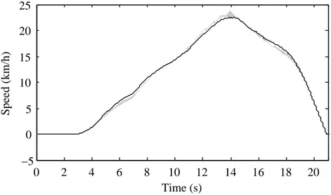
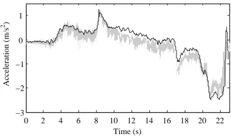
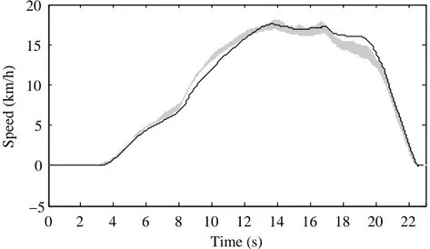
(25) List of Figures 2.1 2.2 2.3 2.4 2.5 2.6 2.7 2.8 2.9 2.10 2.11 2.12 2.13 2.14 2.15 2.16 2.17 2.18 2.19 2.20 2.21 2.22 2.23 2.24 2.25 2.26 2.27 2.28 2.29 2.30 2.31 2.32 2.33 2.34 2.35 2.36 2.37. The National Advanced Driving Simulator . . . . . . . . . . . . Self-developed XBW vehicle prototype . . . . . . . . . . . . . . CAD model of the vehicle prototype . . . . . . . . . . . . . . . Connection scheme: DAS, PC, sensors, actuators, drivers . . . CAD model of the TBW . . . . . . . . . . . . . . . . . . . . . . CAD model of the BBW . . . . . . . . . . . . . . . . . . . . . . Diagram of the SBW system of the XBW vehicle prototype . . CAD model of the rack system for the SBW system . . . . . . CAD model of the wheel torque sensor . . . . . . . . . . . . . . CAD model of a front brake disk . . . . . . . . . . . . . . . . . CAD model of the IMU . . . . . . . . . . . . . . . . . . . . . . CAD model of the steering wheel system . . . . . . . . . . . . . Detailed driver’s force feedback system . . . . . . . . . . . . . . Scheme of the driver’s force feedback system . . . . . . . . . . . Simulink model of the DC motor . . . . . . . . . . . . . . . . . Simulink model of the gearbox . . . . . . . . . . . . . . . . . . Simulink model of the motor friction . . . . . . . . . . . . . . . No load friction curves . . . . . . . . . . . . . . . . . . . . . . . Geared motor with the output shaft blocked . . . . . . . . . . . Elasticity-backlash curve of the gearbox . . . . . . . . . . . . . Locked steering wheel system . . . . . . . . . . . . . . . . . . . Simulink model for the locked steering wheel system . . . . . . Sensor torque, τd , for a sine wave excitation signal . . . . . . . Sensor torque, τd , for a square wave excitation signal . . . . . . Amplifier current, ia , for a sine wave reference . . . . . . . . . . Motor angular velocity, ωm , for a sine wave reference . . . . . . Motor angle, θm , for a sine wave reference . . . . . . . . . . . . Gearbox torque, τg , for a sine wave reference . . . . . . . . . . Gearbox torque, τg , for a square wave reference . . . . . . . . . Motor current, ia , for the free steering wheel case . . . . . . . . Motor angular velocity, ωm , for the free steering wheel case . . Simulink model for the held steering wheel system . . . . . . . Angular velocity of the gearbox, ωm , for the held steering wheel Angle of the gearbox, θg , for the held steering wheel case . . . Motor velocity, ωm , for the held steering wheel case . . . . . . . Motor current, ia , for the held steering wheel case . . . . . . . . Motor voltage, Va , for the held steering wheel case . . . . . . .. xxiii. . . . . . . . . . . . . . . . . . . . . . . . . . . . . . . . . . . . . . . . . . . . . . . . . . . . . . . . . . . . . . . . . . . . . . . . . . . . . . . . . . . . . . . . . . . . . . . . . case . . . . . . . . . . . .. . . . . . . . . . . . . . . . . . . . . . . . . . . . . . . . . . . . . .. . . . . . . . . . . . . . . . . . . . . . . . . . . . . . . . . . . . . .. . . . . . . . . . . . . . . . . . . . . . . . . . . . . . . . . . . . . .. . . . . . . . . . . . . . . . . . . . . . . . . . . . . . . . . . . . . .. . . . . . . . . . . . . . . . . . . . . . . . . . . . . . . . . . . . . .. 9 11 11 13 14 15 16 16 18 18 19 21 21 22 24 25 26 27 28 29 30 30 31 31 32 32 33 34 34 35 35 36 37 37 38 38 39.

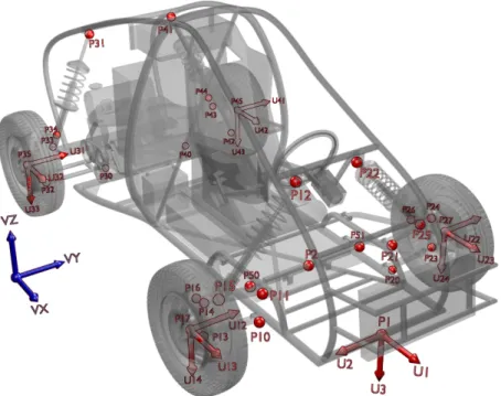
(26) List of Figures. 2.38 2.39 2.40 2.41 2.42 2.43 2.44 2.45 2.46 2.47 2.48 2.49 2.50 2.51 2.52 2.53. Driver’s torque, τd , for the held steering wheel case Brake pressure (straight–line) . . . . . . . . . . . . Throttle angle (straight–line) . . . . . . . . . . . . Longitudinal acceleration (straight–line) . . . . . . Pitch angular velocity (straight–line) . . . . . . . . Right rear wheel torque (straight–line) . . . . . . . Left front wheel speed (straight–line) . . . . . . . . Brake pressure (J–turn) . . . . . . . . . . . . . . . Throttle angle (J–turn) . . . . . . . . . . . . . . . Rack and pinion system angle (J–turn) . . . . . . . Longitudinal acceleration (J–turn) . . . . . . . . . Lateral acceleration (J–turn) . . . . . . . . . . . . Right rear wheel torque (J–turn) . . . . . . . . . . Left front wheel speed (J–turn) . . . . . . . . . . . Roll angular velocity (J–turn) . . . . . . . . . . . . Pitch angular velocity (J–turn) . . . . . . . . . . .. . . . . . . . . . . . . . . . .. . . . . . . . . . . . . . . . .. . . . . . . . . . . . . . . . .. 39 41 41 42 42 43 43 44 44 44 45 45 45 46 46 46. 3.1 3.2 3.3 3.4 3.5 3.6 3.7 3.8 3.9 3.10 3.11 3.12 3.13 3.14 3.15 3.16 3.17 3.18 3.19 3.20 3.21 3.22 3.23 3.24 3.25 3.26 3.27 3.28 3.29. All the points and some vectors of the modeling . . . . . . . . . . . . . . . Points, vectors, COG, reference set of the chassis . . . . . . . . . . . . . . Points, vectors, COG, reference set of the front right lower wishbone arm Points, vectors, COG, reference set of the front right upper wishbone arm Points, vectors, COG, reference set of the front right wheel knuckle . . . . Points, vectors, COG, reference set of the front left lower wishbone arm . Points, vectors, COG, reference set of the front left upper wishbone arm . Points, vectors, COG, reference set of the front left wheel knuckle . . . . . Points, vectors, COG, reference set of the steering system . . . . . . . . . Points, vectors, COG, reference set of the right tie rod . . . . . . . . . . . Points, vectors, COG, reference set of the left tie rod . . . . . . . . . . . . Points, vectors, COG, reference set of the rear right wishbone arm . . . . Points, vectors, COG, reference set of the rear left wishbone arm . . . . . Points, vectors, COG, reference set of the rear right wheel knuckle . . . . Points, vectors, COG, reference set of the rear left wheel knuckle . . . . . Points, vectors, COG, reference set of the front right wheel assembly . . . Points, vectors, COG, reference set of the front left wheel assembly . . . . Points, vectors, COG, reference set of the rear right wheel . . . . . . . . . Points, vectors, COG, reference set of the rear left wheel . . . . . . . . . . Points and vectors for the tire model . . . . . . . . . . . . . . . . . . . . . Approximations of the generalized tire characteristics . . . . . . . . . . . . Longitudinal tire deflection due to the contact forces . . . . . . . . . . . . Lateral tire deflection due to the contact forces . . . . . . . . . . . . . . . Topographical survey with the total station . . . . . . . . . . . . . . . . . 3D scattered points collected during the topographical survey . . . . . . . Interpolation of the 3D scattered points . . . . . . . . . . . . . . . . . . . Contour detection using the alpha shape algorithm . . . . . . . . . . . . . 3D model of the test track . . . . . . . . . . . . . . . . . . . . . . . . . . . Spheres used for the collision detection of the tires . . . . . . . . . . . . .. . . . . . . . . . . . . . . . . . . . . . . . . . . . . .. . . . . . . . . . . . . . . . . . . . . . . . . . . . . .. 51 52 54 55 56 57 58 59 60 60 61 61 62 64 65 66 67 68 69 75 77 77 78 81 82 82 82 83 84. xxiv. . . . . . . . . . . . . . . . .. . . . . . . . . . . . . . . . .. . . . . . . . . . . . . . . . .. . . . . . . . . . . . . . . . .. . . . . . . . . . . . . . . . .. . . . . . . . . . . . . . . . .. . . . . . . . . . . . . . . . .. . . . . . . . . . . . . . . . .. . . . . . . . . . . . . . . . .. . . . . . . . . . . . . . . . .. . . . . . . . . . . . . . . . .. . . . . . . . . . . . . . . . ..

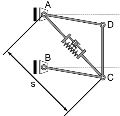
(27) List of Figures. 3.30 3D model of the campus with the skydome in the background . . . . . . . . . 3.31 Photo of the test track . . . . . . . . . . . . . . . . . . . . . . . . . . . . . . . 3.32 3D surroundings of the test track . . . . . . . . . . . . . . . . . . . . . . . . .. 84 85 85. 4.1 4.2 4.3 4.4 4.5 4.6 4.7 4.8 4.9 4.10 4.11 4.12 4.13 4.14. Mean and CI of the rear wheel torques (straight–line) . . . . . . . . . . . . Mean and CI of the brake pressures (straight–line) . . . . . . . . . . . . . . CI and MB model prediction of the left front wheel speed (straight–line) . . CI and MB model prediction of the longitudinal acceleration (straight–line) CI and MB model prediction of the roll angle rate (straight–line) . . . . . . Mean and CI of the rear wheel torque (J–turn) . . . . . . . . . . . . . . . . Mean and CI of the brake pressure (J–turn) . . . . . . . . . . . . . . . . . . Mean and CI of the rack and pinion system angle (J–turn) . . . . . . . . . CI and MB model prediction for the longitudinal acceleration (J–turn) . . . CI and MB model prediction for the lateral acceleration (J–turn) . . . . . . CI and MB model prediction for the left front wheel speed (J–turn) . . . . CI and MB model prediction for the roll angular velocity (J–turn) . . . . . CI and MB model prediction for the pitch angular velocity (J–turn) . . . . CI and MB model prediction for the yaw angular velocity (J–turn) . . . . .. . . . . . . . . . . . . . .. 90 90 91 91 91 92 93 93 93 94 94 94 95 95. 5.1 5.2 5.3 5.4 5.5 5.6 5.7 5.8 5.9 5.10 5.11 5.12 5.13 5.14 5.15 5.16 5.17 5.18 5.19 5.20 5.21 5.22 5.23. Scheme of the 4–bar linkage with a spring–damper element . . . . . . . . Coordinate xD of the 4–bar linkage . . . . . . . . . . . . . . . . . . . . . . Coordinate xD of the 4–bar linkage with the modified penalty formulation 3D model of the Volkswagen Passat . . . . . . . . . . . . . . . . . . . . . Points and vectors for the modeling of the Volkswagen Passat . . . . . . . Model inputs of the Volkswagen Passat . . . . . . . . . . . . . . . . . . . Displacements of the vehicle for an integration time step of 1 ms . . . . . Rotation angles of the vehicle for an integration time step of 1 ms . . . . Displacements of the vehicle for an integration time step of 5 ms . . . . . Rotation angles of the vehicle for an integration time step of 5 ms . . . . UKF: sigma–points for a 2 dimensional GR variable . . . . . . . . . . . . SSUKF: sigma–points for a 2 dimensional GR variable . . . . . . . . . . . Photo of the 5-bar linkage . . . . . . . . . . . . . . . . . . . . . . . . . . . Scheme of the 5–bar linkage . . . . . . . . . . . . . . . . . . . . . . . . . . Angle of the left crank . . . . . . . . . . . . . . . . . . . . . . . . . . . . . Angular velocity of the left crank . . . . . . . . . . . . . . . . . . . . . . . Angular acceleration of the left crank . . . . . . . . . . . . . . . . . . . . . Errors of the filters for the angle of the left crank . . . . . . . . . . . . . . Errors of the filters for the angular velocity of the left crank . . . . . . . . Errors of the filters for the angular acceleration of the left crank . . . . . Errors of the filters for the angle of the left crank . . . . . . . . . . . . . . Errors of the filters for the angular velocity of the left crank . . . . . . . . Errors of the filters for the angular acceleration of the left crank . . . . .. . . . . . . . . . . . . . . . . . . . . . . .. 110 110 111 112 113 113 115 115 116 116 117 118 121 121 122 122 123 124 124 125 125 126 126. xxv. . . . . . . . . . . . . . . . . . . . . . . ..

(28)

(29) List of Tables 2.1 2.2 2.3 2.4 2.5 2.6 2.7 2.8 2.9 2.10. List of the sensors mounted in the vehicle prototype Amplifier parameters . . . . . . . . . . . . . . . . . . Specification of the DC motors – Electrical data . . Identified friction parameters with no load applied . Gearbox elasticity parameters . . . . . . . . . . . . . System component inertias . . . . . . . . . . . . . . Motor parameters . . . . . . . . . . . . . . . . . . . Gearbox parameters . . . . . . . . . . . . . . . . . . Real and simulated rotational velocity . . . . . . . . PI controller parameters . . . . . . . . . . . . . . . .. . . . . . . . . . .. . . . . . . . . . .. 19 23 23 28 29 29 33 33 35 36. 3.1 3.2 3.3 3.4 3.5 3.6 3.7 3.8 3.9 3.10 3.11 3.12 3.13 3.14 3.15 3.16 3.17 3.18 3.19 3.20 3.21. Chassis mass properties . . . . . . . . . . . . . . . . . . . . . . . . . . . . . COG coordinates and inertia tensor for the chassis . . . . . . . . . . . . . . COG coordinates and inertia tensor for the front right lower wishbone arm COG coordinates and inertia tensor for the front right upper wishbone arm COG coordinates and inertia tensor for the front right wheel knuckle . . . . COG coordinates and inertia tensor for the front left lower wishbone arm . COG coordinates and inertia tensor for the front left upper wishbone arm . COG coordinates and inertia tensor for the front left wheel knuckle . . . . . COG coordinates and inertia tensor for the steering system . . . . . . . . . COG coordinates and inertia tensor for the rear right wishbone arm . . . . COG coordinates and inertia tensor for the rear left wishbone arm . . . . . COG coordinates and inertia tensor for the rear right wheel knuckle . . . . COG coordinates and inertia tensor for the rear left wheel knuckle . . . . . COG coordinates and inertia tensor for the front right wheel . . . . . . . . Front left wheel mass properties . . . . . . . . . . . . . . . . . . . . . . . . . COG coordinates and inertia tensor for the front left wheel . . . . . . . . . Rear right wheel mass properties . . . . . . . . . . . . . . . . . . . . . . . . COG coordinates and inertia tensor for the rear right wheel . . . . . . . . . Rear left wheel mass properties . . . . . . . . . . . . . . . . . . . . . . . . . COG coordinates and inertia tensor for the rear left wheel . . . . . . . . . . Summary of variables and constraints . . . . . . . . . . . . . . . . . . . . .. . . . . . . . . . . . . . . . . . . . . .. 53 53 54 55 56 57 58 59 60 62 62 63 65 66 67 67 68 69 69 70 72. 5.1 5.2 5.3 5.4. Color code for the figures of the 4–bar linkage . . . CPU times for the 4–bar linkage simulations . . . . CPU time and number of iterations for ∆t = 1 ms Color code for the figures of the 5–bar linkage . . .. . . . .. 111 111 114 122. xxvii. . . . .. . . . . . . . . . .. . . . .. . . . . . . . . . .. . . . .. . . . . . . . . . .. . . . .. . . . . . . . . . .. . . . .. . . . . . . . . . .. . . . .. . . . . . . . . . .. . . . .. . . . . . . . . . .. . . . .. . . . . . . . . . .. . . . .. . . . . . . . . . .. . . . .. . . . . . . . . . .. . . . .. . . . . . . . . . .. . . . .. . . . . . . . . . .. . . . .. . . . ..

(30) List of Tables. 5.5. CPU times and RMSE . . . . . . . . . . . . . . . . . . . . . . . . . . . . . . . 125. xxviii.

(31) List of Datasheets Data acquisition system – DAP4200a . . . . . . . . . . . . . . . . . . . . . . Custom command of the TBW system . . . . . . . . . . . . . . . . . . . . . Custom command of the BBW system . . . . . . . . . . . . . . . . . . . . . Custom command for the RWM of the SBW system . . . . . . . . . . . . . Custom command for the SWM of the SBW system . . . . . . . . . . . . . Encoder of the TBW – HEDS 5540 A06 . . . . . . . . . . . . . . . . . . . . Encoder of the TBW – 3100R0040G0LB00 . . . . . . . . . . . . . . . . . . Torque sensor of the SBW – TFF 350 - FSH00646 . . . . . . . . . . . . . . Signal conditioner for the torque sensor of the SBW – CSG110 - FSH01449 Wheel torque sensor – 90360 . . . . . . . . . . . . . . . . . . . . . . . . . . Hall effect sensor – 1GT101DC . . . . . . . . . . . . . . . . . . . . . . . . . Accelerometer – CXL02LF3 . . . . . . . . . . . . . . . . . . . . . . . . . . . Gyroscope – CRS03-02 . . . . . . . . . . . . . . . . . . . . . . . . . . . . . . Inclinometer – SCA121t . . . . . . . . . . . . . . . . . . . . . . . . . . . . . Current sensor – CSNS300 . . . . . . . . . . . . . . . . . . . . . . . . . . . . Stepper motor of the TBW – 23HSX-206 . . . . . . . . . . . . . . . . . . . Gearbox of the TBW – MRIG02 . . . . . . . . . . . . . . . . . . . . . . . . Driver of the TBW – PM546 . . . . . . . . . . . . . . . . . . . . . . . . . . Linear actuator of the BBW – DRL60PB4-05G . . . . . . . . . . . . . . . . Indexer of the BBW – CN0173 . . . . . . . . . . . . . . . . . . . . . . . . . Driver of the BBW – DFC5114T . . . . . . . . . . . . . . . . . . . . . . . . DC motor of the SBW – M66CI 500 L-24 . . . . . . . . . . . . . . . . . . . Gearbox for the DC motors of the SBW – IP57-M2-50 . . . . . . . . . . . . Servo-amplifier for the DC motors of the SBW – ADSE 50-5 . . . . . . . . Servo-amplifier for the DC motors of the SBW – MSE421 . . . . . . . . . . Total station for the topographical survey – Sokkia SET530R . . . . . . . .. xxix. . . . . . . . . . . . . . . . . . . . . . . . . . .. . . . . . . . . . . . . . . . . . . . . . . . . . .. . . . . . . . . . . . . . . . . . . . . . . . . . .. . . . . . . . . . . . . . . . . . . . . . . . . . .. 133 139 141 143 145 149 151 153 155 157 159 161 163 165 167 171 173 175 179 181 183 185 187 189 191 195.

(32)

(33) Acronyms AC AL. alternating current. 20 augmented Lagrangian. 48, 49. BBW. brake-by-wire. Brake-by-wire systems are electronically controlled braking systems. 11, 14, 15, 40, 42, see XBW. CAD CDKF CEMF CI COG CPR CPU. computer-aided design. 10, 11, 15, 17, 53, 82–84 central difference Kalman filter. A SPKF variant. 100, see SPKF counter electromotive force. 36, 38 confidence interval. 89, 90, 92, 96 center of gravity. 53–71 number of full quadrature cycles per full shaft revolution (360 mechanical degrees). 16 central processing unit. 111, 114, 123, 125. DAE DAS DC DOF. differential algebraic equation. 3, 48, 49, 100, 102, 103 data acquisition system. 12, 14–18, 21, 34, 40, 53, 81, 113, 129 direct current. 15, 19–21, 23, 26, 30, 33, 38, 128 degrees of freedom. 52–64, 66, 68, 70–72, 103, 112–114, 128. EKF. extended Kalman filter. Kalman filter for nonlinear systems that linearizes about the current mean and covariance. 5, 100, 104, 105, 108, 109, 111, 112, 114, 117–119, 122–125, 128, 129. FE FM FT. finite element. 74 frequency modulation. 17 field testing. xxxv, xxxvii–xxxix, 8–10, 17. GRV. Gaussian random variable. 105. HIL HITL. hardware-in-the-loop. 3 human-in-the-loop. 3. I3AL IMU. index 3 augmented Lagrangian. 48 inertial Measurement Unit. Electronic device fitted with acceleration, velocity and orientation sensors. 19. KF. Kalman filter. A mathematical method (recursive estimator) named after Rudolf E. Kálmán.. xxxv–xxxix, 100, 103–105, 114. LIM LKF. Laboratorio de Ingenierı́a Mecánica. 2, 4, 5, 81 linearized Kalman Filter. 100. xxxi.

(34) Acronyms. LRKF. linear regression Kalman filter. This name is sometimes used for the SPKF. 100. MB. multibody. xxxv–xxxix, 2–5, 9, 10, 17, 18, 48, 54, 57, 71, 73–75, 80–84, 89, 90, 92, 96, 97, 100, 102–105, 109, 111, 112, 114, 117, 120, 122, 125, 128, 129. NADS NVH. National Advanced Driving Simulator. A high-fidelity driving simulator situated at the University of Iowa. 4, 8, 9, 128 Noise Vibration and Harshness. 74. ODE. ordinary differential equation. 49, 101, 103–105, 108. PC PI PID PM PSU. personal computer. 12, 129 proportional-integral. A PI controller is a control loop-feedback controller. 22, 36 proportional-integral-derivative. A PID controller is a control loop-feedback controller. 16, 17 permanent magnet. 15, 20, 23, 38, 128 power supply unit. It supplies current to computer’s components. 12. RHS RK2 RMSE RWM. right–hand side. 107 Runge–Kutta 2 method. A second order explicit integrator. 104, 119, 122, 125 root mean squared error. 123, 125 road wheel motor. Actuator that steers the wheels of a vehicle equipped with a SBW system. 15–17, see SBW. SBW. steer-by-wire. Steer-by-wire systems are electronically controlled steering systems. 5, 11, 15–17, 19, 20, 38, 42, 128, 129, see XBW sigma-point Kalman filter. 5, 100, 104, 111, 114, 123, 124, 128 spherical simplex unscented Kalman filter. A SPKF variant based on the unscented transform. 100, 114, 119, 120, 122, 125, see SPKF & UKF steering wheel motor. Actuator that generates a driver’s force feedback for a SWS system. 15–17, 19, 20, see SWS steering wheel system. Driver’s force feedback system for SBW systems. xxxv–xxxix, see SBW. SPKF SSUKF SWM SWS. TBW TR. throttle-by-wire. Throttle-by-wire systems are systems that control electronically the throttle pedal or valve. 11, 14, 40, 42, see XBW trapezoidal rule. A second order implicit integrator. 104, 106, 108, 119, 120, 122, 125. UKF. unscented Kalman filter. A SPKF variant based on the unscented transform. 100, 114, 117, 119, 120, 122, 125, see SPKF. VDANL. Vehicle Dynamics Analysis, Non-Linear. Vehicle dynamics simulation code developed by Systems Technology, Inc.. 8 Vehicle Dynamics Models for Roadway Analysis and Design. Vehicle dynamics simulation code developed by the University of Michigan – Transportation Research Institute. 8 Vehicle Research and Test Center. This is an American federal research facility. 9. VDM Road VRTC XBW. X-by-wire. X-by-wire systems refer to systems controlled electronically (brake-by-wire, throttleby-wire...) in contrast to the traditional systems controlled mechanically. 9, 10, 15, 17, 20, 40, 48, 71, 75, 89, 128, 129. ZOH. zero–order hold. 123. xxxii.

(35) Acronyms. xxxiii.

(36)

(37) Glossary In the whole document, the following typesetting rules for the mathematical notation have been adopted: • vectors and matrices are in upright and bold types • scalars are in italics and normal font types • each glossary entry is followed by one of these three abbreviation: FT for field testing notation, SWS for the notation related to the steering wheel system, MB for the multibody notation or KF for the Kalman filtering notation. Notation. α. Description radial stiffness tire coefficient (MB) coefficient of the differential equation of the longitudinal deflection of the tire (MB) coefficient of the differential equation of the longitudinal deflection of the tire (MB) coefficient of the differential equation of the longitudinal deflection of the tire (MB) primary scaling factor defining the extension of the spread of the sigma–points around the mean of the estimates (KF) penalty factors (MB). α1 α2 α3 α10 α20 α30. load load load load load load. b1. coefficient of the differential equation of the lateral deflection of the tire (MB) coefficient of the differential equation of the lateral deflection of the tire (MB) coefficient of the differential equation of the lateral deflection of the tire (MB) scaling factor used to control the weighting of the zeroth sigma– point (KF) constant parameter for the viscous term of the gearbox torque τg . Unit: A (SWS). 79, 80. C χ cx cy. damping matrix (MB) sigma–point (KF) longitudinal stiffness coefficient of the tire (MB) lateral stiffness coefficient of the tire (MB). 49, 106–109 117–119 78–80 78–80. d ∆ti. radial tire damping coefficient (MB) integration time step (MB). 76 79, 80, 122, 125. a a1 a2 a3 α. b2 b3 β bg. dependent dependent dependent dependent dependent dependent. coefficient coefficient coefficient coefficient coefficient coefficient. for for for for for for. the the the the the the. gearbox. Unit: gearbox. Unit: gearbox. Unit: motor. Unit: – motor. Unit: – motor. Unit: –. xxxv. N m−1 (SWS) N m−1 (SWS) s/N m (SWS) (SWS) (SWS) (SWS). Page List 76 79, 80 79 79, 80 117, 118 48–50, 111 26, 28, 26, 28, 26, 32, 26, 28, 26, 28, 26, 32,. 103, 104, 108– 32, 32, 33 32, 32, 33. 33 33 33 33. 79, 80 79, 80 118 24, 25, 33.

(38) Glossary. Notation. ∆ts dx dy. Description update time step of the sensors (KF) longitudinal damping coefficient of the tire (MB) lateral damping coefficient of the tire (MB). Page List 122, 123, 125 78–80 78–80. en ex ey eyR ezR. contact normal (MB) unit vector giving the direction of the longitudinal tire force (MB) unit vector giving the direction of the lateral tire force (MB) unit vector defining the wheel plane (MB) unit vector defining the wheel orientation (MB). 74, 74, 74, 74, 74. f. dynamics system function (KF). F F. linearization of the dynamics system function (KF) Function that expresses the dependent acceleration as function of the dependent coordinates and velocities (MB) tire force. Unit: N m (SWS) friction force. Unit: N m (SWS) Coulomb friction level. Unit: N m (SWS) level of the stiction force. Unit: N m (SWS) vertical force of the tire. Unit: N (MB). 101, 104, 105, 107– 109 101, 105, 107, 109 103, 104. F F Fc Fs Fz g. 75 75 75 75. 76–80 26, 27 25–27 25–27 76. nonlinear function to be solved using Newton–Raphson scheme (MB) coupling matrix between process noise and the state of a linear dynamic system (KF) tire camber angle. Unit: rad (MB) scaling factor defining the extension of the spread of the sigma– points around the mean of the estimates (KF). 49, 50, 106–109. H. linearization of the measurement sensitivity matrix (KF). h. measurement sensitivity matrix (KF). 101, 102, 105, 106, 108, 109 101, 102, 105–107, 118. i. index used for iterative processes (MB and KF) motor’s armature current. Unit: A (SWS) average current drawn by the motor. Unit: A. (SWS) current reference given by the digital acquisition processor. Unit: A. (SWS) reference current for the amplifier. Unit: A (SWS) lower bound of idap . Unit: A (SWS) upper bound of idap . Unit: A (SWS). 48–50, 106 22, 23, 34, 36, 37 27 22, 34. inertia of the gearbox. Unit: kgm2 (SWS) inertia of the coupling. Unit: kgm2 (SWS) sum of the inertia of the gearbox and the coupling inertia. Unit: kgm2 (SWS) inertia of the DC motor. Unit: kgm2 (SWS) inertia of the steering wheel. Unit: kgm2 (SWS) inertia at the output shaft of the gearbox: Jg + Jsw . Unit: kgm2 (SWS). 29 29 25, 29. k. index used to indicate the time step (MB and KF). K. stiffness matrix (MB). 49, 50, 101, 102, 104, 106–109, 117–120 49, 106–109. G γ∗ γ. ia iavg idap iref i− sat i+ sat J1 J2 Jg Jm Jsw Jtot. xxxvi. 101, 102, 105 75 117. 22, 23, 34 22, 23 22, 23. 23, 25, 29 25, 29 25.

(39) Glossary. Notation. k1 k2 κ K̄. Description coeff. when |iref | < |ia |. Unit: Ω (SWS) Coeff. when sign(iref ) 6= sign(ia ). Unit: Ω (SWS) user–defined tuning parameter for the UKF (KF) Kalman gain matrix (KF). kg1 kg3 kg5 Ki km,avg Kp ks kv. constant parameter for the gearbox. Unit: N m/rad (SWS) constant parameter for the gearbox. Unit: N m/rad3 (SWS) constant parameter for the gearbox. Unit: N m/rad5 (SWS) integral coefficient for PI or PID controllers. Unit: N (SWS) DC motor torque constant. Unit: N m/A (SWS) proportional coefficient for PI or PID controllers. Unit: N (SWS) stiffness of the torque sensor. Unit: N m/rad (SWS) DC motor voltage constant. Unit: V/rad/s (SWS). L L La. 50, 51, 54–63, 65, 70 117–119 23. λ λ. distance between two points. Unit: m (MB) dimension of the state vector (KF) leakage inductance in the armature winding of the DC motor. Unit: H (SWS) parameter of the UKF (KF) vector of Lagrange multipliers (MB). M m M. wheel center coordinates (MB) number of Lagrange multipliers (MB) positive definite mass matrix (MB). 75 48 48, 49, 102–111. n n nd ni. sample number (FT) gearbox ratio (ωin /ωout ) (SWS) number of dependent coordinates (MB) number of independent coordinates (MB). nsp ν νn νs νx νx∗ νy νy∗. number of sigma–points (KF) velocity of displacement (SWS) small velocity used to avoid numerical problems (SWS) Stribeck velocity (SWS) longitudinal velocity of the contact point (MB) modified tangential velocity of the tire tread (MB) lateral velocity of the contact point (MB) modified tangential velocity of the tire tread (MB). 89 24, 25, 33 48, 103, 104 103–105, 107, 112, 114 117–119 26, 27 76, 78, 80 26–28, 33 75–80 78, 79 75–80 78–80. Ω ω ωm. wheel angular velocity (MB) natural frequencies of the constraints for the penalty formulation (MB) DC motor angular velocity. Unit: rad/s (SWS). 76, 78–80 48, 103, 104, 108, 109, 111 23, 32, 34, 37. P P. geometric contact point coordinates (MB) covariance matrix of state estimation uncertainty (KF). Φ φ. linearization of the state transition matrix (KF) state transition matrix (KF). Φ. vector of constraints (MB). φ. angle between two vectors or segments. Unit: rad (MB). 74, 75 101, 102, 105, 106, 117, 118 102 101, 102, 117, 118, 120 48–50, 102–104, 108– 111 50, 51, 54–59, 61–63, 65–70, 72, 73, 120. xxxvii. Page List 22, 23 22, 23 117 101, 102, 105–109, 111, 118–120 24, 29 24, 29 24, 29 36 23, 27 36 30 23. 117, 118 48, 49, 102, 103. 108,.

(40) Glossary. Notation. Q Q q R. Description vector containing the external forces, the velocity–dependent inertia forces and those obtained from a potential (MB) covariance matrix of the process noise (KF) vector of dependent coordinates (MB). Page List 48, 49, 102–109, 111 101, 102, 105 48–50, 102–104, 107– 111, 120 103, 105–108, 120. rD. matrix defining a basis of the nullspace of the Jacobian matrix of the constraints (MB) covariance matrix of measurement uncertainty (KF) reference point coordinates. Unit: m (MB) resistance of the armature winding of the DC motor. Unit: Ω (SWS) dynamic rolling radius. Unit: m (MB). s sc S sg σ0 σ1 σ2 ŝx sx ŝy sy. varying distance. Unit: m (MB) critical generalized slip. Unit: - (MB) sample standard deviation (FT) generalized slip. Unit: - (MB) stiffness of the bristles. Unit: N m (SWS) damping coefficient of the bristles. Unit: N m/rad/s (SWS) damping coefficient. Unit: N m/rad/s (SWS) normalizing factor for the longitudinal slip (MB) longitudinal slip. Unit: - (MB) normalizing factor for the lateral slip (MB) lateral slip. Unit: - (MB). 51, 70–72, 109–111 76, 79, 80 89 76, 78–80 26–28, 32, 33 26, 27 26–28 76, 78 76, 78–80 76, 78 76, 78–80. t t. student’s t distribution (FT) time (MB and KF). τd τfg. driver’s torque acting on the steering wheel. Unit: Nm (SWS) friction torque that models the friction between the inner gears of the second stage and the ring gear of the two stage planetary gearbox. Unit: Nm (SWS) friction between the shaft and the armature as well as the friction between the inner gears of the first stage and the ring gear of the two stage planetary gearbox. Unit: Nm (SWS) friction force without load. Unit: Nm (SWS) gearbox’s torque. Unit: Nm (SWS) elastic term of the gearbox torque. Unit: Nm (SWS) viscous term of the gearbox torque. Unit: Nm (SWS) motor’s torque. Unit: Nm (SWS) twist of the gearbox. Unit: rad (SWS). 89 48–50, 101, 103–109, 123 25, 36 25, 27. R r Ra. τfm τf,no−load τg τg elastic τg visc τm θa θ̇a θg θ̈g θm θ̈m. 101, 102, 105 50–52, 54–63, 65, 70 23 76, 78, 79. 23, 25, 27. 27 25, 24, 24, 23, 24. 26 25 25 25. first derivative of the twist of the gearbox. Unit: rad/s (SWS) gearbox angle. Unit: rad (SWS). 24 24, 36. second derivative of the gearbox angle. Unit: rad/s2 (SWS) motor angle. Unit: rad (SWS). 25 24, 32, 36. second derivative of the motor angle. Unit: rad/s2 (SWS). 25. u. unit vector (MB). 50–59, 61–63, 65–72. v. vector containing the coordinate vector and its first time– derivative (MB) measurement noise vector (KF) voltage of the motor. Unit: V (SWS) motor’s voltage lower bound. Unit: V (SWS). 104. v Va − Vsat. xxxviii. 101, 102, 105, 118 22, 23, 34–37 23.

(41) Glossary. Notation + Vsat. Description motor’s voltage upper bound. Unit: V (SWS). Page List 22, 23, 34. w. process noise vector (KF). w W w. weight for the SPKFs (KF) weight of the objective function for the projections (MB) vector of dependent velocities (MB). 101, 102, 105, 118, 120 118, 119 49, 50 104–109, 111. x x x. sample (FT) Cartesian coordinate (MB) state vector (KF). ẋe xe xe0. longitudinal tire deflection velocity (MB) longitudinal tire deflection (MB) initial longitudinal tire deflection for each integration time step (MB). Y y y. sigma–point propagated through the measurement sensitivity matrix (KF) Cartesian coordinate (MB) measurement vector (KF). ẏe ye ye0. lateral tire deflection velocity (MB) lateral tire deflection (MB) initial lateral tire deflection for each integration time step (MB). ζ. damping ratios of the penalty formulation (MB). z z z. average deflection of the bristles (SWS) vertical deflection of the tire. Unit: m (MB) independent coordinate vector (MB). xxxix. 89 109, 120 89, 101, 102, 105–110, 117–119 77–80 78–80 79, 80. 118 109, 120 101, 102, 105–108, 111, 118–120, 123 77–80 78–80 79, 80 48, 103, 104, 108, 109, 111 26, 27 76 103–108, 119, 120.

(42)

(43) Chapter 1. Introduction. 1.

(44) 1. Introduction. 1.1. Motivations. Vehicle dynamics has been a privileged field of application of mechanics for decades. Before the advent of personal computers in the 1970s, vehicle dynamics were only studied in analytical form due to the mathematical limitations in solving large problems. Until that date, vehicle models remained relatively simple as they had to be expressed in closed-form. Since then, computer performances and multibody (MB) simulations have substantially improved. Vehicle MB models and simulation software to analyze vehicle dynamics rapidly appeared in the 1980s to make up for the lack of comprehensive vehicle models (Körtum, 1985). These models have gained in complexity and accuracy to include some behaviors, characteristics of vehicle components and subsystems that were not considered previously. As a consequence of this evolution, the vehicle dynamics field has divided into application sub-fields such as for instance vehicle real-time simulations, handling analysis or ride comfort analysis. The Laboratorio de Ingenierı́a Mecánica (LIM) of the University of La Coruña has specialized in real-time MB simulations. Real-time vehicle dynamics is one of its application fields. Natural coordinates and a self-developed MB formulation that enables the simulation of complex systems to run in real-time with efficiency and robustness (Naya et al., 2007) are the preferred choices to model vehicles in the LIM. This thesis pretends to gain new insights into this research line. In practice, reliability and validity which are major concerns when developing vehicle models, must be investigated for the vehicle modeling methods developed in the LIM. Indeed, it is essential to check the correctness of the implementation and to adjust the level of accuracy of the model to the application requirements. In the automotive domain, this implies vehicle field testing to gather experimental data that is then compared to the predictions of the simulation. A. H. Hoskins clearly formulated the need for validation claiming that “Without validation of the vehicle dynamics there is only speculation that a given model accurately predicts a vehicle response” (Hoskins and El-Gindy, 2006). Nowadays simplified vehicle models are commonly employed in on-board stability controllers (Tseng et al., 1999). The next step in the evolution of these controllers should be the use of validated real-time MB models. This can be compared to the past evolution of vehicle dynamics simulations from classical vehicle models to MB models. The use of real-time vehicle MB models in state observers is a research subject recently initiated at the LIM. Using state estimation techniques and highly-detailed vehicle models should provide information to the controllers that is not available when using classical vehicle models. The substitution of classical vehicle models by MB models is not trivial. Both theory and implementation aspects need to be deeply investigated.. 1.2. State of the art of multibody analysis in the automotive field. In the last decade, MB analysis has become a standard to speed up the development process of vehicles (Fischer, 2007; Lugner and Plöch, 2004; Rauh, 2003). The reduction in cost, risk and time during the development is one of the most relevant contributions of MB techniques. MB models are not intended to replace vehicle models from the classical vehicle dynamics theory (Gillespie, 1992; Jazar, 2008; Wong, 2001) but to augment the range of the vehicle models. Vehicle models are at present divided into several groups that are employed at different stages of the vehicle development process. Rauh (2003) identified four groups. The. 2.

(45) 1.2 State of the art of multibody analysis in the automotive field. first, called partial aspect models, roughly describes certain aspects of the motion of the vehicle or the behavior of certain parts of the vehicle. The second group, named behavior models, outlines the main characteristics of the vehicle dynamics. The third group is made of 3D functional models which allow to simulate the overall vehicle behavior and normally take into account inputs of the driver, 3D motion, four wheels, suspension elements, etc. The last group, composed of 3D component oriented models, is the specific field of MB models. These highly detailed models represent each individual component based on its physical properties. The more detailed the model is, the more accurate the simulation predictions of the future vehicle dynamics are. In light of this classification, MB models do not appear to replace classical vehicle models but to widen the range of vehicle models. Literature that links MB books and classical vehicle dynamics books is slowly appearing (Blundell and Harty, 2004; Popp and Schielhen, 2010). MB models are built either using self-developed specific tools and methods that guarantee efficiency and customizability, or using commercial MB softwares allowing greater ease of use at the expense in most cases of adaptability to new requirements and end-product integration. Typical MB softwares are SIMPACK from SIMPACK AG, ADAMS from MSC or even Virtual.Lab Motion from LMS . It is worth mentioning that MB models in the automotive industry have five different objectives that imply different modeling strategies: handling analysis, ride analysis, durability analysis, real-time applications and crash analysis. It should also be mentioned that due to the continuous improvement of computer performances and MB formulations, MB vehicle models are being used in more and more automotive subfields previously reserved to classical vehicle models. The five objectives are discussed hereafter. The first three objectives (handling, ride and durability analysis) have similar model requirements. Vehicle handling analysis, the most common objective, aims at characterizing the vehicle dynamics. Ride analysis focuses on ride comfort while the objective of durability analysis is to improve the service life of vehicle components. For these analysis, real-time execution is not required but accuracy and ease of use are essential. Numerous MB models (self-developed or developed using commercial MB software) have been developed following these objectives. They are highly detailed models that normally include all the vehicle components with their nonlinear characteristics in order to quantitatively characterize the vehicle nonlinear behavior. The equations of motion of the vehicle are generally a set of differential algebraic equation (DAE). Since variable step size integration schemes adapt themselves to the system natural frequencies, they are commonly used to guarantee accurate solutions. As listing exhaustively all the MB models that were developed up to now for handling, ride and durability analysis would be a highly intensive task, a selection of relevant scientific papers is presented below instead. Hegazy et al. (2000) presented a 94 degrees of freedom nonlinear MB model. This model takes into consideration all the compliance sources. MB models with flexible chassis were developed using flexible MB formulations (Ambrósio and Goncalves, 2001; Cuadrado et al., 2004b). Rill (2006b) presented vehicle modeling by subsystems. Aerodynamic interactions were taken into account by Hussain et al. (2007) for a 102 degrees of freedom nonlinear MB model. The fourth objective of MB models is related to real-time simulations. These simulations are used in human-in-the-loop (HITL) applications like high fidelity driving simulators or in hardware-in-the-loop (HIL) applications like component behavior evaluation systems. Real-time full-vehicle MB models can be built following two different approaches: complete. 3.