Quantitative assessments of geometric errors for rapid prototyping in medical applications

Texto completo

(1)PONTIFICIA UNIVERSIDAD CATOLICA DE CHILE SCHOOL OF ENGINEERING. QUANTITATIVE ASSESSMENTS OF GEOMETRIC ERRORS FOR RAPID PROTOTYPING IN MEDICAL APPLICATIONS. CRISTÓBAL ARRIETA. Thesis submitted to the Office of Research and Graduate Studies in partial fulfillment of the requirements for the degree of Master of Science in Engineering. Advisor: CRISTIÁN TEJOS. Santiago de Chile, March 2011 c MMXI, C RIST ÓBAL A RRIETA ⃝.

(2) PONTIFICIA UNIVERSIDAD CATOLICA DE CHILE SCHOOL OF ENGINEERING. QUANTITATIVE ASSESSMENTS OF GEOMETRIC ERRORS FOR RAPID PROTOTYPING IN MEDICAL APPLICATIONS. CRISTÓBAL ARRIETA. Members of the Committee: CRISTIÁN TEJOS PABLO IRARRÁZAVAL ALEX VARGAS LUCIANO CHIANG Thesis submitted to the Office of Research and Graduate Studies in partial fulfillment of the requirements for the degree of Master of Science in Engineering Santiago de Chile, March 2011 c MMXI, C RIST ÓBAL A RRIETA ⃝.

(3) To Alejandro Arrieta.

(4) ACKNOWLEDGEMENTS. This work was supported by Fondecyt 1100864 and, Anillo ACT79 and FONDEF D06I1026. I give my most sincere thanks to the person without whom I would have been unable to work on this thesis, nor embark on this new path in my life. He is my academic advisor Cristian Tejos. His guidance, concern and dedication were invaluable, as it was his constant encouragement to give my best. I have come to deeply admire him as a teacher and researcher. After all these months, I am glad I can also count him as a very good friend. I also would like to thank to my parents, Victor Hugo y Lorena, and my brothers, Daniel and Gabriel, whose constant support was crucial in order to finish this thesis. I cannot forget to mention my friends, Felipe, Ivan, Gonzalo and Tomas. They have always been there, to celebrate and share the joy of the good days and to bring the support I needed on those who were not as good. I specially thank Camila, whose deep impact in my life led me to where I am now. A thesis itself would be required to explain how, so for the sake of brevity I just will say that I am greatly grateful for her role in my life. Finally, I would like to thank my colleagues at the Biomedical Imaging Center. Firstly, to my partner of work and laugh, with whom I have shared topics beyond professional issues, Carlos Sing-Long. Secondly, to Pablo Irarrazaval, whose scientific rigor and honesty, no matter how hard the truth sounds, are both admirable and very inspiring. And finally to Sergio Uribe, Vicente Parot, Jose Luis Honorato, Allan Cid and Carlos Milovic, as this thesis has contributions, in one form or another, from all of them.. iv.

(5) TABLE OF CONTENTS. ACKNOWLEDGEMENTS . . . . . . . . . . . . . . . . . . . . . . . . . . . . . . .. iv. LIST OF FIGURES . . . . . . . . . . . . . . . . . . . . . . . . . . . . . . . . . . .. vi. ABSTRACT . . . . . . . . . . . . . . . . . . . . . . . . . . . . . . . . . . . . . . .. vii. RESUMEN . . . . . . . . . . . . . . . . . . . . . . . . . . . . . . . . . . . . . . .. viii. . . . . . . . . . . . . . . . . . . . . . . . . . . . . . . . . .. 1. 2. MATERIALS AND METHODS . . . . . . . . . . . . . . . . . . . . . . . . . .. 5. 2.1. RP models construction . . . . . . . . . . . . . . . . . . . . . . . . . . . . .. 5. 2.2. Data processing of RP models . . . . . . . . . . . . . . . . . . . . . . . . .. 7. 2.3. Global accuracy metric . . . . . . . . . . . . . . . . . . . . . . . . . . . . .. 8. . . . . . . . . . . . . . . . . . . . . . . . . . . . . .. 9. 3. RESULTS . . . . . . . . . . . . . . . . . . . . . . . . . . . . . . . . . . . . . .. 13. 3.1. Phantom results . . . . . . . . . . . . . . . . . . . . . . . . . . . . . . . . .. 13. 3.2. Bone results . . . . . . . . . . . . . . . . . . . . . . . . . . . . . . . . . . .. 14. 3.3. Sensitivity analysis . . . . . . . . . . . . . . . . . . . . . . . . . . . . . . .. 16. 4. DISCUSSION . . . . . . . . . . . . . . . . . . . . . . . . . . . . . . . . . . . .. 21. References . . . . . . . . . . . . . . . . . . . . . . . . . . . . . . . . . . . . . . . .. 25. GLOSARY . . . . . . . . . . . . . . . . . . . . . . . . . . . . . .. 27. 1. INTRODUCTION. 2.4. Local accuracy metric. APPENDIX A.. v.

(6) LIST OF FIGURES. 1.1 Examples of ambiguities in landmark-based error methods. . . . . . . . . . . . . .. 3. . . . . . . . . . . . . . . . . . . . . . . . . . . . . . . . .. 5. 2.2 Examples of RP models built from cadaveric bones. . . . . . . . . . . . . . . . . .. 6. 2.3 Graphic descriptions of global indexes. . . . . . . . . . . . . . . . . . . . . . . .. 9. 2.4 Calculating the signed normal distance. . . . . . . . . . . . . . . . . . . . . . . .. 11. 3.1 ACWE segmentation of the phantoms . . . . . . . . . . . . . . . . . . . . . . . .. 13. . . . . . . . . . . . . . . . . . . . . . . . .. 14. 3.3 ACWE segmentation of the ulna . . . . . . . . . . . . . . . . . . . . . . . . . . .. 14. 3.4 ACWE segmentation of the metacarpal 2 . . . . . . . . . . . . . . . . . . . . . .. 15. 3.5 ACWE segmentation of the metacarpal 2 . . . . . . . . . . . . . . . . . . . . . .. 15. 3.6 ACWE segmentation of the metacarpal 3 . . . . . . . . . . . . . . . . . . . . . .. 16. 3.7 Global error representation . . . . . . . . . . . . . . . . . . . . . . . . . . . . . .. 16. 3.8 Local error representation . . . . . . . . . . . . . . . . . . . . . . . . . . . . . .. 17. 3.9 Sensitivity analysis varying λ2 (bone) . . . . . . . . . . . . . . . . . . . . . . . .. 19. 3.10Sensitivity analysis varying λ2 (RP model) . . . . . . . . . . . . . . . . . . . . .. 20. 2.1 Analytical phantoms.. 3.2 ACWE segmentation of the humerus. vi.

(7) ABSTRACT. Rapid Prototyping (RP), a technology for producing three dimensional (3D) models or replicas of objects of interest, has become an important tool for surgical planning, prosthesis manufacturing, and assisting diagnosis. Crucial for these medical applications is the geometric accuracy of RP models. Current research on evaluating the geometric accuracy of RP has focused in identifying two or more specific anatomical landmarks on the original object and the RP model, and comparing their corresponding linear distances. Such kind of accuracy metrics is ambiguous and may induce misrepresentation of the actual errors. As an alternative accuracy metric, we propose to use two different approaches: (1) the formulation of a global accuracy evaluation using volumetric intersection indexes calculated over segmented Computed Tomography scans of the original object and the RP model, and (2) the formulation of a local error metric that is computed from the surfaces of the original object and the RP model. This local error is rendered in a 3D surface using a color code, that allow differentiating regions where the model is over estimated, under estimated, or correctly estimated. Global and local error measurements involve a rigid body registration based on the maximization of Mutual Information, a segmentation based on the Active Contours Without Edges algorithm, volumetric calculations based on the segmented images, triangulations based on Marching Cubes algorithm, and local calculations based on the triangulations. Our results show that our procedures can be applied without any modification to different objects, and provide simple and meaningful quantitative indexes to measure the volumetric accuracy of models built with RP technology.. Keywords: Rapid prototyping, geometric accuracy, volumetric accuracy indexes, active contours. vii.

(8) RESUMEN. El Prototipado Rápido (PR), tecnologı́a utilizada para construir modelos tridimensionales (3D) o réplicas de objetos, ha tomado gran importancia en aplicaciones médicas, especialmente para planificación de cirugı́as, diseño de prótesis y docencia. La precisión geométrica de los modelos PR es esencial para estas aplicaciones médicas. El método más común para evaluar la precisión geométrica es identificar puntos anatómicamente relevantes en el objeto original y en el modelo PR y comparar las distancias lineales entre pares de puntos correspondientes. Este tipo de métrica sufre de ciertas ambigüedades y puede llevar a una mala medición del error. Como método alternativo para medir el error, proponemos dos enfoques: (1) Generar una métrica para evaluar la precisión global, usando ı́ndices que comparen los volúmenes de la estrutura original y el modelo PR, calculados sobre imágenes de Tomografı́a Computarizada, y (2) Generar una métrica para evaluar la precisión local, comparando las superficies del objeto original y del modelo PR. El error local se muestra en una representación 3D de la superficie usando un código de colores, lo que permite diferenciar las regiones sobre estimadas, subestimadas o correctamente estimadas. Las mediciones del error global y local requieren del uso de una etapa de registro utilizando Información Mutua, segmentación usando el algoritmo Active Contours Without Edges, cálculo de los ı́ndices volumétricos sobre las segmentaciones, triangulación usando el algoritmo Marching Cubes, y cálculo del error local sobre las triangulaciones. Los resultados muestran que el método propuesto se puede aplicar en diferentes objetos sin ningún cambio, demostrando ser una herramienta que provee ı́ndices volumetricos simples y representativos de la precisión geométrica con que modelos PR son construidos.. Palabras claves: Prototipado rápido, precisión geométrica, ı́ndices de precisión volumétricos, contornos activos. viii.

(9) 1. INTRODUCTION. Rapid Prototyping (RP) is a technique that was introduced in mechanical engineering for producing three-dimensional (3D) physical models of objects. RP is used in medical applications to construct realistic replicas of biological structures (also known as RP models), being the most common application the construction of bone models. RP models have been used for surgical planning, prosthesis design, assisted diagnosis, and teaching purposes (Choi et al., 2002; Silva et al., 2008; Schicho et al., 2006; Russett et al., 2007; Ngan et al., 2006). The construction of RP models typically consists of four steps. (1) The object to be modeled is scanned using a volumetric medical imaging technique, typically Computed Tomography (CT) or Magnetic Resonance Imaging (MRI). (2) The object of interest is segmented out from the acquired image. (3) The object of the segmented structure is triangulated to generate a piece-wise continuous surface model, which is then exported into an STL (STereoLitography) file. (4) The model is built from the STL file using one of the existing RP techniques. Unfortunately, each step of this process introduces several errors (e.g. voxelation, segmentation errors, piecewise linear smoothing by the triangulation, deformations due to calibration errors of the printer), so the resulting RP model is not geometrically identical to the object. The accuracy of RP models is crucial in medical applications, hence, having a reliable error metric is essential to evaluate the final product. Most of the documented methods use linear distances between anatomical landmarks to quantify these geometric errors (Choi et al., 2002; Silva et al., 2008; Schicho et al., 2006; Russett et al., 2007; Nizam et al., 2006; Knox et al., 2005; El-Katatny et al., 2010). For example, Choi et al. (2002) implemented a procedure by identifying two or more relevant anatomical landmarks and locating them on the object and on the corresponding places in the RP model. They measured the linear distances between landmarks in the object and compared these distances to the ones obtained from the RP model. Despite their extensive use, landmark-based error methods have three disadvantages: Firstly, they require an experienced person who needs to identify manually and precisely a set of relevant anatomical features for the specific object. There are significant intra-observer. 1.

(10) and inter-observer differences placing the landmarks. In order to alleviate intra-observer effects, Choi et al. (2002) and Silva et al. (2008) needed to average over 20 different distance measurements of each landmark pair in their RP accuracy studies. Mallepree and Bergers (2009) proposed a method to measure the accuracy of RP models using a Coordinate Measuring Machine (CMM) that measures 23 landmark pairs with 6 iterations per measurement. Although they improved the degree of automatism of the landmarking process, intra-observer reproducibility is still an issue as they require several iterations for each measurement. Solutions to the inter-observer variability have not been discussed so far in the literature. Secondly, even if landmarks are perfectly located, error metrics based on linear distances would still suffer from inherent ambiguities and could lead to wrong conclusions when they are used to quantify volumetric errors. Figure 1.1 shows some examples of these ambiguities. For instance, if in the RP model two landmarks are erroneously displaced in the same direction and same magnitude with respect to the original object (Figure 1.1 (a)), the distance between them would not change, so no error would be detected. Alternatively, if only one of landmark is misplaced (Figure 1.1 (b)), the method would detect an error, but without identifying which landmark is in the wrong position. Another ambiguity occurs depending on where the RP model is measured. For instance, an overestimated doughnut-like object (Figure 1.1 (c)) would present an increased linear distance (2R + α) in the outer diameter whereas the inner diameter would show a decreased linear distance (2r − α), despite of the underlying geometric error being the same. Thirdly, when landmark-based methods are used to encode global geometric errors (i.e. a number that represents the total error of the RP model), the common approach is to take the mean and standard deviation of the differences between an arbitrarily chosen number of landmark distances. This produces an unfair comparison between different objects since the number of landmarks tend to vary across objects. In summary, landmark-based methods have intrinsic and inevitable ambiguities, and result in error estimates that, depending on the object, the type of distortions and the number of measurements, could be inaccurate.. 2.

(11) (a). (b). (c) F IGURE 1.1. Examples of ambiguities in landmark-based error methods. I every example, solid and dashed lines correspond to the original object and the RP model, respectively. (a) If the landmarks of the RP model are erroneously displaced in the same magnitude and direction, no error would be detected as the measured distance would not change. (b) When only one of the those landmarks are misplaced, the measured distance would reflect that there is a geometric error in the RP model, but it would not be possible to establish which of the two landmarks is the erroneous one. (c) A single kind of distortion can lead to different types of measurements, depending on where the model is measured. Comparing the inner diameter of a doughnut-like object would show a decreased linear distance, whereas comparing the outer diameter would show an increased linear distance.. Recently, Germani et al. (2010) proposed a slightly different accuracy evaluation method that considered a colored surface representation to show local errors. The colors represented the local error of the RP models computed as the magnitude of the distance to the nearest point between two overlapped point clouds. Consequently, they did not give information about the direction of these errors, so that it is not possible to know whether the resulting RP models are overestimated or underestimated. 3.

(12) Considering these issues, we propose two different approaches to deal with the global (indexes that represent the total error of the RP model) and local (error distribution along the surface of the RP model) geometric error quantification. For global accuracy, we propose to use volumetric intersection indexes computed over scans of the object and the RP model. The purpose of this is twofold: to provide a more accurate measure of error by simple and meaningful indexes that take into account volumes, avoiding thus the ambiguities present in methods based on linear distances; and to privilege automation, as only little human intervention is needed. For local accuracy, we propose to use a 3D surface map with a color code that indicates if each region of the RP model overestimates, underestimates, or correctly estimates the surface of the original object. Furthermore, by means of an intensity code, we are able to quantify the local error in each region of the RP model.. 4.

(13) 2. MATERIALS AND METHODS. In this section, we present our method for the analysis of geometric errors in RP models. Firstly, we show how the RP models were constructed. We made experiments with cadaveric bones and phantoms in which we controlled the geometric errors. Secondly, we describe the different steps to acquire and process the data. Finally we present how the global and local metrics are computed.. 2.1. RP models construction We generated two analytical phantoms, designed with the software CATIAT M v.5 R14 (Dassault Systèmes, Vélizy-Villacoublay, France): (1) a sphere with radius 2.5cm (Figure 2.1 (a)), and (2) a sphere with the same radius with two cylindrical defects, one of them added volume (Figure 2.1 (b)) and the other subtracted the same volume (Figure 2.1 (c)), so as to keep the same volume of the original sphere. The radius of both cylinders was 0.7cm. The height of one of them was 1cm and we found the other height by preserving the sphere volume, resulting in a slightly smaller height. The added and subtracted volumes were equal to 1.478cm3 , i.e. 2.26% of the total volume.. (a) Original sphere.. (b) Sphere with two cylindrical defects (the defect that adds volume is shown).. (c) Sphere with two cylindrical defects (the defect that subtracts volume is shown).. F IGURE 2.1. Analytical phantoms.. 5.

(14) We also built RP models of cadaveric bones obtained from the Department of Anatomy of our University. For our experiments we used 5 bones: a humerus portion, an ulna, and three metacarpal bones. Two examples are shown in Figure 2.2.. (a) Metacarpal bone 1. (b) Metacarpal bone 2. F IGURE 2.2. Examples of RP models built from cadaveric bones.. The RP models were constructed from CT scans (GE HiSpeed Dual) obtained with the following parameters: 80kV, 80mA, matrix resolution of 512 × 512 and slice thickness of 1mm. The field of view was adjusted on each experiment so that to optimize the in-plane image resolution. Data were processed using a standard software application for RP models (MimicsT M 12, Materialise, Leuven, Belgium). This software has a manually thresholding-based segmentation and some basic region growing-based tools to edit the results of the segmentation. From this segmentation, the software generated a triangulated surface, which was exported as an STL file. The STL was exported into the ZPrintT M software, re-sliced with resolution of 0.08mm and built in an arbitrarily chosen geometric orientation, using a ZPrinterT M Spectrum 510 system (ZCorporation, MA, USA). For our experiments, the RP models were not infiltrated. To run blind experiments, an independent operator performed the whole RP building process of all the studied objects. This operator did not participate in the evaluation process, which will be described in the following sections. 6.

(15) 2.2. Data processing of RP models Once the RP model was constructed, we performed a CT scan of the RP model with the same parameters of the object. We used these parameters as they showed the best results in terms of image quality. At this point we had two sets of medical images, one from the object and another from the RP model. In order to have voxel to voxel spatial correspondence, we registered both CTs using a rigid body algorithm based on mutual information (Wells, Viola, & Kikinis, 1996) available in the software application SPM (http://www.fil.ion.ucl.ac.uk/spm, accessed on 17 January 2011). The registered images were segmented using a 3D Active Contour Without Edges (ACWE) algorithm (Chan & Vese, 2001) implemented in a home-made application using MATLAB 7.8.0 (Mathworks, Natick, Massachusetts, USA). This is a level set-based segmentation technique, which is formulated using a Mumford-Shah functional (Mumford & Shah, 1989). Basically, the image is divided into two regions and the interface of these regions will evolve in order to define two homogeneous regions. This is solved minimizing the energy functional. F (c1 , c2 , C) = µ · Area(C) + ν · Volume(inside(C)) + ∫ λ1 |u0 (⃗x) − c1 |2 d⃗x + inside(C). ∫. (2.1). |u0 (⃗x) − c2 |2 d⃗x,. λ2 outside(C). where C corresponds to the surface that describes the interface, u0 (⃗x) corresponds to the 3D image, c1 and c2 are the average intensity of u0 inside and outside of C, respectively. Additionally, µ, ν, λ1 and λ2 are fixed parameters chosen by the user and they represent the weights of each term in the objective function. The first term of the equation 2.1 forces the surface C to be smooth. The second term minimizes the volume inside C, but having a minimal volume is not usually desired so typically ν = 0. The third and fourth terms force C to be located such that the interior and exterior regions are as homogeneous as possible.. 7.

(16) The minimization of equation 2.1 is achieved by an iterative method (Chan & Vese, 2001) consisting of a finite difference discretization in the spatial domain and a forward Euler time discretization which adds a ∆t parameter that represents the size of one time step of this method. After a few tests in one slice of a bone and RP model, we set the parameters as: µ = 0.01 · 2552 , ν = 0, λ1 = 1, λ2 = 7 (bone), λ2 = 1 (RP model), ∆t = 0.01, 300 iterations, 9 iterations of reinitialization after the first iteration and then every 101 iterations. We kept these parameters constant for all our experiments. The only human intervention was the initialization process, which consisted in defining an ellipsoid that surrounded the entire object of interest. Once the segmentation process ended, automatic morphological operations are needed to extract only the exterior surface of the analyzed object. Finally, we generated a triangulated surface and STL files of both data sets using the marching cubes algorithm (Lorensen & Cline, 1987).. 2.3. Global accuracy metric Using the segmented images from the object and the RP model we analyzed the global geometric error using three indexes (Figure 2.3). The first index A was the normalized intersection between voxels that belong to the object segmentation Vb and to the RP model segmentation Vm : ∑ (Vb ∩ Vm ) ∑ A= · 100. Vb. (2.2). We defined the normalized False Positive error (F P ), i.e. voxels that appears in the the RP model segmentation but not in the object segmentation (Ṽb ), as: ∑ (Ṽb ∩ Vm ) ∑ FP = · 100, Vb. (2.3). and the normalized False Negative (F N ) error, i.e. voxels that appears in the object segmentation but not in the RP model segmentation (Ṽm ), as: 8.

(17) ∑ (Vb ∩ Ṽm ) ∑ FN = · 100. Vb. (2.4). F IGURE 2.3. Graphic descriptions of global indexes. The left and right figures represent the voxels of the object and the RP model, respectively. Gray voxels correspond to the intersection (A, Eqn. 2.2), pink voxels correspond to the false positives (FP, Eqn. 2.3) and purple voxels to the false negatives (FN, Eqn. 2.4).. 2.4. Local accuracy metric Using the surface triangulation of the object and the RP model, we analyzed the local geometric errors. The idea was to have an indication of how far apart were those surfaces. We compared both triangulations computing a signed normal distance of each triangle of the object to the nearest triangle of the RP model. The surface of the model could be overestimated (positive distance), underestimated (negative distance) or well-estimated (zero distance). Each of these classifications had a corresponding color, pink tones for F P , purple tones for F N , and gray for well estimated regions. Then, the intensity was associated with the magnitude of the signed normal distance. That information was rendered in a 3D representation of the object. To compute the signed normal distances we proceeded as follows (Figure 2.4): 1.- Compute Is and Im , the incenter of the triangles of the object and RP model, respectively. 2.- Compute n̂s and n̂m , the unit outer normal of the triangles of the object and RP model, respectively. 3.- Compute the plane that contains each triangle of the RP model as 9.

(18) ax + by + cz + d = 0,. (2.5). where a, b and c are known since n̂m = (a, b, c) and d is defined as. d = −n̂m • I⃗m ,. (2.6). where • is the dot or inner product. 4.- Define ⃗s, the normal straight line of each triangle of the object through Is as. ⃗s = I⃗s + t · n̂s ,. (2.7). where t is a free parameter. 5.- Compute the intersection point P between ⃗s and the plane that contains each triangle of the RP model. This can be done evaluating equation 2.7 with t equals to:. t=. −d − I⃗s • n̂m . n̂s • n̂m. (2.8). 6.- Keep the intersection points P that belong to the interior of any triangle of the RP model and discard the rest. We considered that edges and vertices belonged to the interior of the triangles. 7.- Compute the signed normal distances as. D = ∥Is − P ∥ · sign(t),. (2.9). where ∥·∥ is the Euclidean distance, sign(t) = 1 denotes an outer normal direction and sign(t) = −1 denotes an inner normal direction. 8.- As each ⃗s usually intersects more than one triangle, we simply chose the distance D with the smallest magnitude (Dm ). At this stage each triangle of the object surface has a corresponding signed normal distance Dm . 10.

(19) F IGURE 2.4. Calculating the signed normal distance. The yellow triangles represent the RP model surface and the green triangle represent the object surface. The red arrow represents the straight line in the normal direction and the green arrow represents the straight line in the opposite normal direction. Is represents the incenter of the object triangle and P represents intersection between the normal straight line and the RP model triangulated surface. D represents the distance between Is and P , which is positive because is in the normal direction. It would be negative if the intersection was in the opposite normal direction.. 9.- Generate a color code of 256 levels to show each Dm with a corresponding color. The Red, Green and Blue (RGB) channels of the color code were defined as follows: (a) Find the level that corresponds to the zero distance with the proportion:  p = f loor 256 ·. ⃗ m) min(D ⃗ m) ⃗ m ) + max(D min(D.  ,. ⃗ m is the vector that contains the signed normal distances of all the triangles that belong where D to the object and the function f loor rounds to the nearest integers towards minus infinity. (b) The p − th element, corresponding to the zero signed normal distance, was defined as gray RGB = [0.45 0.45 0.45]. We needed that the colormap gradually changes its color for negative and positive distances, so we assigned the blue channel for the negative distances and the red 11.

(20) channel for the positive distances. (c) For negative distances we defined the 256 elements of the blue channel using equation 2.10:    B(i) =. 0.55 ⃗ m) min(D. + 0.45 i = 1 . . . p.  0.45. (2.10) i = p + 1 . . . 256.. (d) For positive distances we defined the red channel using equation 2.11:. R(i) =.   0.45  . 0.55 ⃗ m) max(D. i = 1...p − 1. (2.11). + 0.45 i = p . . . 256.. (e) The green channel of the colormap was G = 0.45 for all values. Different color codes can be constructed by simply adjusting the coefficients of the straight lines defined in equations 2.10 and 2.11.. 12.

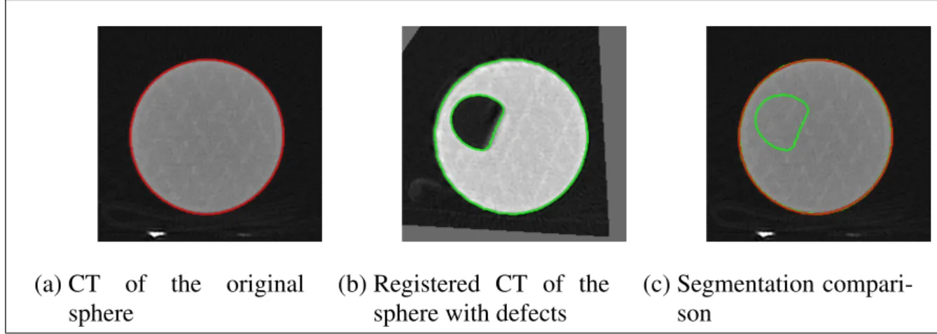
(21) 3. RESULTS. 3.1. Phantom results Figure 3.1 shows the result of the registration and the ACWE segmentation of the original sphere and the sphere with cylindrical defects. Figure 3.1 (c) shows the superposition of the segmentation represented by contours. The segmentation algorithm based on ACWE worked equally well on the original sphere (red contour in Figure 3.1 (a)) and on the sphere with defects (green contour in Figure 3.1 (b)). By superposing both segmentations together (red and green contours) onto the CT of the original sphere (Figure 3.1), it can be seen that there is no substantial differences between them, except in the region of the introduced defect.. (a) CT of the original sphere. (b) Registered CT of the sphere with defects. (c) Segmentation comparison. F IGURE 3.1. 3D ACWE segmentation of the phantoms. Only one slice is shown. The red and the green contour show the ACWE segmentation of the original sphere and the sphere with cylindrical defects, respectively. The only difference between the segmentations is the added defect.. The global accuracy indexes of the spheres were: A = 97.17%, F P = 2.48% and F N = 2.83%. Whereas the expected indexes were 97.74% and F P = F N = 2.26%. The local error is shown in Figure 3.8(a). The region in red represents the introduced false positive cylinder defect. The maximum and minimum signed normal distances are about 6mm and -6mm, respectively. This slight underestimation is probably due to the voxelation effects. 13.

(22) 3.2. Bone results As can be seen from Figures 3.2, 3.3, 3.4, 3.5 and 3.6, the registration and segmentation worked well for all CT scans. Figure 3.7 shows the global errors of each bone. It can be seen that there is a slight geometric error in the RP models, as there is a consistent overestimation in their sizes. Indeed, the amount of false positives is greater than the amount of false negatives, except in the metacarpal 3.. (a) Bone. (b) RP model. (c) Segmentation comparison. F IGURE 3.2. 3D ACWE segmentation of the humerus portion. Only one slice is shown. The red and the green contour show the ACWE segmentation of the bone and the RP model, respectively.. (a) Bone. (b) RP model. (c) Segmentation comparison. F IGURE 3.3. 3D ACWE segmentation of the ulna. Only one slice is shown. The red and the green contour show the ACWE segmentation of the bone and the RP model, respectively.. 14.

(23) (a) Bone. (b) RP model. (c) Segmentation comparison. F IGURE 3.4. 3D ACWE segmentation of the metacarpal 1. Only one slice is shown. The red and the green contour show the ACWE segmentation of the bone and the RP model, respectively.. (a) Bone. (b) RP model. (c) Segmentation comparison. F IGURE 3.5. 3D ACWE segmentation of the metacarpal 2. Only one slice is shown. The red and the green contour show the ACWE segmentation of the bone and the RP model, respectively.. These percentages of false positives (Figure 3.7) represent the global accuracy of RP models but they do not show information about where these errors are located. Figure 3.8 shows our local error representation. As previously stated, pink tones represent over estimated regions (F P ), purple tones, under estimated regions (F N ) and gray tones, correctly estimated regions. Except for the metacarpal 3, most of the rendered surfaces show F P errors. This is consistent with the computed global indexes. Moreover, in general the F N are concentrated on specific zones of the surface. The result of the metacarpal 3 is different since the F P and F N are equally distributed along the surface, which is also consistent with the global error results. 15.

(24) (a) Bone. (b) RP model. (c) Segmentation comparison. F IGURE 3.6. 3D ACWE segmentation of the metacarpal 3. Only one slice is shown. The red and the green contour show the ACWE segmentation of the bone and the RP model, respectively.. (a) Geometric accuracy (A). (b) Geometric errors (F P ) and (F N ).. F IGURE 3.7. Global error representation. Geometric accuracy of the RP models measured as normalized intersection (A) between original structures and RP models and geometric errors of the RP models measured as normalized false positive errors (F P ) and false negative errors (F N ).. 3.3. Sensitivity analysis We were interested in evaluating the impact in varying the segmentation parameters in the global error calculation. As mentioned in section 2.2, we used the same parameters for the object and RP model segmentation, except for λ2 which is the most sensitive one. We therefore did a sensitivity analysis varying each λ2 in ±10% (Figures 3.9 and 3.10) and calculating the indexes A, F P and F N . We tested our results with the humerus data sets. 16.

(25) (a) Phantom RP model. (b) Humerus RP model.. (c) Cubit RP model.. (d) Metacarpal 1 RP model.. (e) Metacarpal 2 RP model.. (d) Metacarpal 3 RP model.. F IGURE 3.8. Local error representation. The rendering shows the signed normal distances represented by a color code specified by the colorbar at the right hand side of each figure (in millimeters).. 17.

(26) Changes in λ2 for the RP model segmentation produced larger variations than for the object segmentation (Figure 3.10 (c)). However, variations were always less than 0.05% of the total volume of the object.. 18.

(27) (a) Intersection variation (A). (b) False positive variation (F P ). (c) False positive variation (F N ) F IGURE 3.9. Sensitivity analysis varying the segmentation parameter λ2 of the object.. 19.

(28) (a) Intersection variation (A). (b) False positive variation (F P ). (c) False negative variation (F N ) F IGURE 3.10. Sensitivity analysis varying the segmentation parameter λ2 of the RP model.. 20.

(29) 4. DISCUSSION. We have developed a methodology for measuring the accuracy of RP models with a reasonably degree of automation. Indeed, the entire evaluation process was done without any human intervention except from the ellipsoid initialization of segmentation. The computed indexes are a simple and meaningful way to observe the degree of global accuracy and the geometric errors of the built RP model. Moreover, as a complementary metric, we generated a local error representation that indicates how the error is distributed along the RP model surface. The results show that both metrics are consistent. For the construction of RP accuracy indexes it is necessary to establish correspondence between the objects of interest and their RP models. Until now, such problem had been faced by trying to establish corresponding landmarks (sometimes referred as fiducials) on each structure and applying a rigid body (Euclidean) transformation to them. However, landmarking processes are labor-intensive and heavily depends on the ability of the operator to define those corresponding points (Maes et al., 1997). In general, the resulting correspondence between external fiducials is poor (Meyer et al., 1996). Furthermore, measuring a few landmarks does not give a good representation of the accuracy of complex shapes, and local representations of errors are needed (Germani et al., 2010). We propose an alternative solution as there is substantial evidence that spatial correspondence can be achieved by searching the rigid body transformation that maximizes the Mutual Information between images (Meyer et al., 1996; Maes et al., 1997). The method is robust even when there are intensity differences between the images that are being registered. This is exactly our case as the image intensities of bones and RP models are shown differently in the CT scans. An additional justification to move away from landmark-based error metrics, is their inherent ambiguity. As we showed, there are some situations where such metrics cannot detect evident errors, they cannot discriminate the exact location of the errors or, depending where is measured, they show differently a single kind of error.. 21.

(30) Another important point is the chosen segmentation. We believe that a significant portion of the geometric errors that we found in the RP models was produced by the thresholdingbased segmentation algorithm. The threshold-based segmentations have the problem that Choi et al. (2002) called the dumb-bell-like effect. Basically, choosing a smaller threshold than the ideal value adds a volume layer, whereas choosing a larger threshold than the correct one subtracts a volume layer. This is an inevitable drawback, especially in bone segmentation, since the detection of trabecular bone in most cases implies an overestimation of cortical bone. In this scenario, we proposed the use of an active contour-based segmentation, which is semiautomatic, robust to the noise and combines geometric and intensity constraints. Thus, this method shows advantages compared to the threshold-based ones and allows us to make a fair comparison between two structures that have different intensities. From the computed results, it is interesting to observe that the RP models tend to overestimate the size of the original bone structure. In fact, the global accuracy indexes show that the F P are consistently greater than the F N , except for the metacarpal 3. This might be due to the small size of this bone, particularly in the slice direction. This might increase the significance of the voxelation and volume averaging effects. The local representation of error adds relevant information to geometric accuracy evaluations. The most important conclusions are two. On one hand, the amount of underestimated surface, i.e. the F N (see the color bar in the right side of the Figures 3.8) was usually concentrated in particular regions. On the other hand, the amount of over estimated surface, i.e. F P (surface of pink color in Figures 3.8), was distributed along most of the surface, which confirms the results given by global indexes. An important contribution of our method is that it not only quantifies the error, but also shows where the error is located. This is an important issue for medical applications, such as surgery or prosthesis design, since geometric accuracy is particularly relevant at specific regions where the object interacts with other structures. There are several sources that could explain these errors, those derived from the scanning process (e.g. voxelation, volume averaging effects and reconstruction artifacts); those derived from the pre-processing stage (e.g. errors from the segmentation process, and from the surface. 22.

(31) triangulation); and those derived from the manufacturing process (e.g. miscalibration, voxelation effects and re-slice and building orientation). Our methodology also introduces additional sources of errors, such as potential misalignments obtained from the registration process, image interpolations involved in the registration process, and segmentation errors derived from the chosen segmentation algorithm (ACWE). However, the results with synthetic phantoms show that these additional sources of errors are bounded and do not significantly affect our metric results. Indeed, the phantoms were built synthetically by software, so they do not contain errors from construction process (at least from the CT scan, segmentation and triangulation), and the computed error did not showed significant differences with the synthetically introduced errors. With our method for quantitative assessment of geometric errors we have the tools to judge the accuracy of eventual improvements for the construction process. In an image processing context, we believe that efforts to improve the accuracy of RP models should be focused on the application of more adequate segmentation strategies to process the tomographic images of the original objects to be modeled. The segmentation tools available in standard RP software applications (thresholding and region growing) offer great advantages in terms of speed and simplicity, but they inevitably introduce segmentation errors. Indeed, they are not robust to noise and other commonly encountered artifacts in medical images. Moreover, those algorithms involve choosing heuristically the magnitude of the thresholds, which potentially introduces biases as in medical imaging, the image contrast typically varies across the field of view due to image artifacts. Importantly, our proposed method can be used to evaluate other RP technologies or other applications. We are currently working on controlling the topology of the segmenting contour, such as in (Han, Xu, & Prince, 2003), so that to avoid the morphological corrections needed for the ACWE algorithm. This would simplify and improve robustness of the segmentation process.. 23.

(32) References. Chan, T. F., & Vese, L. A. (2001). Active contours without edges. IEEE Transaction on Image Processing, v. 10, 266–277. Choi, J., Choi, J., Kim, N., Kim, Y., Lee, J., Kim, M., et al. (2002). Analysis of errors in medical rapid prototyping models. International Journal of Oral and Maxillofacial Surgery, v. 31, 23–32. El-Katatny, I., Masood, S., & Morsi, Y. (2010). Error analysis of FDM fabricated medical replicas. Rapid Prototyping Journal, v. 16, 36–43. Germani, M., Raffaeli, R., & Mazzoli, A. (2010). A method for performance evaluation of RE/RP systems in dentistry. Rapid Prototyping Journal, v. 16, 344–355. Han, X., Xu, C., & Prince, J. L. (2003). A topology preserving level set method for geometric deformable models. IEEE Transactions on Pattern Analysis and Machine Intelligence, v. 25, 755–768. Knox, K., Kerber, C., Singel, S., Bailey, M., & Imbesi, S. (2005). Stereolithographic vascular replicas from CT scans: choosing treatment strategies, teaching, and research from live patient scan data. American Journal of Neuroradiology, v. 26, 1428–1431. Lorensen, W. E., & Cline, H. E. (1987). Marching cubes: A high resolution 3D surface construction algorithm. Computer Graphics, v. 21, 163–169. Maes, F., Collington, A., Vandermeulen, D., Marchal, G., & Suetes, P. (1997). Multimodality image registration by maximization of mutual information. Medical Image Analysis, v. 16, 187–198. Mallepree, T., & Bergers, D. (2009). Accuracy medical RP models. Rapid Prototyping Journal, v. 5, 325–332. Meyer, C., Boes, J., Kim, B., Zasadny, P. B. K., Kison, P., Koral, K., et al. (1996). Demonstration of accuracy and clinical versatility of mutual information for automatic multimodality image fusion using affine and thin-plate spline warped geometric deformations. Medical Image Analysis, v. 1, 195–206.. 24.

(33) Mumford, D., & Shah, J. (1989). Optimal approximations by piecewise smooth functions and associated variational problems. Communications on Pure and Applied Mathematics, v. 42, 577–685. Ngan, E., Rebeyka, I., Ross, D., Hirji, M., Wolfaardt, J., Seelaus, R., et al. (2006). The rapid prototyping of anatomic models in pulmonary atresia. The Journal of Thoracic and Cardiovascular Surgery, v. 132, 264–269. Nizam, A., Gopal, R., Naing, L., Hakim, A., & Samsudin, A. (2006). Dimensional accuracy of the skull models produced by rapid prototyping technology using stereolithography apparatus. Orofacial Sciences, v. 1, 60–66. Russett, S., Major, P., Carey, J., Toogood, R., & Boulanger, P. (2007). An experimental method for stereolithic mandible fabrication and image preparation. The Open Biomedical Engineering Journal, v. 1, 1–8. Schicho, K., Fogl, M., Seeman, R., Ewers, R., Lambrecht, J., Wagner, A., et al. (2006). Accuracy of treatment planning based on stereolithograpphy in computed assited surgery. Medical Physics, v. 33, 3408–3417. Silva, D., Oliveira, M. G. de, Meurer, E., Meurer, M., Silva, J. L. da, & Santa-Barbara, A. (2008). Dimensional error in selective laser sintering and 3D-printing of models for craniomaxillary anatomy reconstruction. Journal of Cranio-Maxillofacial Surgery, v. 36, 443–449. Wells, W., Viola, P., & Kikinis, R. (1996). Multi-modal volume registration by maximization of mutual information. Medical Image Analysis, v. 1, 35–51.. 25.

(34) APPENDIX A. GLOSARY. CAD: Computer Aided Design. CT: Computed Tomography. MRI: Magnetic Resonance Imaging. Phantom: Is an object designed and developed in order to evaluate or calibrate medical imaging devices. Registration: In an image processing context, registration is the process of referencing two or more sets of images into a common coordinate system, in order to have a voxel-to-voxel correspondence between all the images. RP: Rapid Prototyping. Segmentation: In an image processing context, segmentation is the process of extract or isolate an object of interest from an image that has several objects. STL: STereoLithography, is a file format for CAD softwares that contains a triangulation description. Triangulation: In an image processing context, triangulation is the process of transforming a voxel-based representation of a volumetric image into a polygon-based representation, specifically a set of triangles and vertices that lie in three dimensional space. Voxel: Is the minimal volumetric element of a three dimensional grid. Voxel is the analogous of a pixel in two dimensional images.. 26.

(35)