Determination of the distribution of shallow water seagrass and drift algae communities with acoustic seafloor discrimination
10
0
0
Texto completo
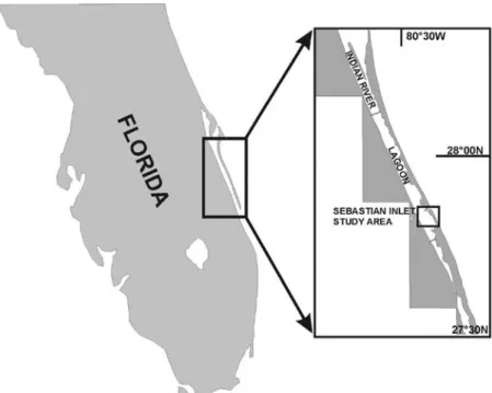
(2) Fig. 1. Study areas in the Indian River Lagoon, Florida, USA.. system on a 50 and a 200 kHz signal frequency to detect boundaries of areas covered by seagrass and drift algae in shallow waters of mostly less than 2 m depth. MATERIAL AND METHODS The QTC View Series V system is a sonar-based hydrographic survey unit and accompanying software suite that can provide acoustic habitat classifications based on the interpreted shape of direct-incidence echoes reflected from the seafloor (Collins et al. 1996, Collins and Lacroix 1997). The classification system has been shown to perform well in shallow water settings (Hamilton et al. 1999, Preston et al. 2000, 2002), and provides seafloor discrimination based on the diversity of responses (subsurface reverberation, specular and diffuse backscatter) of different seafloor types. Bottom types will influence the shape of a returning echo, for example, a smooth bottom, or flat growth form will return a first echo with a smooth shape while a rough, complicated bottom, or branching growth form 166. will return a more convoluted echo shape with a correspondingly higher degree of backscatter (Collins et al. 1996, Preston et al. 2000). Depth artefacts are avoided by automatic gain control and proprietary algorithms expanding on the work of Chivers et al. (1990), Prager et al. (1995) and Collins et al. (1996). Echoes returning from the seafloor are digitized, and using the QTC Impact software decomposed by a suite of algorithms into 166 variables (Fourier analysis producing 64 variables, wavelet analysis producing 64 variables, kurtosis, surface area, and others; Legendre 2002, Legendre et al. 2002). Series of four consecutive echoes are “stacked” in order to provide an “average” wave-form (called a full-feature-vector, or FFV) with lower susceptibility to random noise and signal variation. In the next step, the first three principal components of a PCA are used to ordinate the signals in three-dimensional space where a Baysian clustering routine then assigns similarity groupings. The number of clusters is decided on by the operator (QTC 2000, Legendre et al. 2002). The process has been critically reviewed and discussed by Hamilton et al. (1999), Hamilton (2001),. Rev. Biol. Trop. (Int. J. Trop. Biol. ISSN-0034-7744) Vol. 53 (Suppl. 1): 165-174, May 2005 (www.tropiweb.com).
(3) Legendre (2002) and Legendre et al. (2002) as well as Preston et al. (2002). The QTCView Series 5 system was used in conjunction with a Suzuki ES 2025 depth sounder operating at 50 and 200 kHz at a ping rate of 10 Hz and a fixed, omnidirectional transducer with an opening angle of 42º (50 kHz) and 12º (200 kHz). Transmit power was regulated through an autogain control feature in the software QTC View, which avoided signal saturation. The typical process of benthic habitat classification using QTC View involves a boatbased survey that acquires acoustic data that are then converted from analog to digital. During data collection, each acoustic trace is time-stamped and later merged with navigation data. After the survey, data are checked for correct time-stamps, depths and signal strengths. All signals that do not pass an appropriate level of quality control are discarded. Prior to attempting any calibration or examining the patterns near Sebastian Inlet, it was necessary to see whether any patterns based on the acoustic signal classification could be discerned at all. The data obtained were subjected to classification procedures in the software QTC Impact (Anonymous 2000) and split to a level of four classes which were known to be present in the study area: bare substratum, seagrass, dense algae, sparse algae. After the field survey, data were classified and the areas in between the survey lines were filled by using spatial statistics methods. The most plausible spatial prediction was obtained by nearest-neighbor interpolation after resampling the irregular survey grid to a regular grid. To provide evidence that the classifications of field underway-survey data reflected reality and that echo-groupings were not misinterpreted, calibration was undertaken using the same bottom categories. At first, calibration was attempted directly in the study area where the survey vessel was positioned over discreet known habitat patches (seagrass, dense algae, sparse algae, bare substratum) where datasets containing about 1500 echo traces were obtained. Then, the boat was anchored. over an area of bare substratum, drift algae were collected and placed in various densities underneath the transducer on the anchored, stable vessel. Two densities of drift algae were used (250 g m-2, 2000 g m-2). On each of the experimental plots, individual datasets of about 1500 echo traces were recorded. To assure that this process really detected the algae and was reliable, algae were collected and returned to the laboratory. At the university marina in Fort Lauderdale, which opens into the Intracoastal Waterway and therefore has comparable salinity and temperature to the Indian River lagoon (which is situated further to the north along the intracoastal waterway), the transducer was suspended from the edge of a pier over 2 m of muddy seafloor. A wire-basket of a size sufficient to cover the entire footprint (calculated as r=depth.tanθ/2, where θ is the transducer opening angle) was suspended over a 1.8 m deep seafloor directly underneath the transducer at variable distance between transducer and basket. Files of about 1500 traces were obtained with the empty basket, basket with 250 g m-2 and basket with 2000 g m-2 algae. This procedure was repeated in 1.3 m and 0.7 m depth. Additionally, separate files with different settings of blanking depth and signal length (parameters to be set in QTC View software) were obtained to evaluate whether these factors had any influence on groupings. During each individual trial, signal properties were held constant and only files obtained with identical signal properties were compared. To evaluate the accuracy of the acoustic ground discrimination, ground-truthing transects consisting of geo-referenced images obtained by video drop-camera were collected. The habitat types observed in the videos were then compared to those from the gridding and extrapolation analysis. Accuracy of the maps was then assessed using a confusion matrix approach (Mumby and Green 2000). An Atlantis AUW-5600 color underwater camera was used to capture video images along the survey lines. The video signal was time stamped and merged with positioning information from a handheld GPS unit. Video survey data were. Rev. Biol. Trop. (Int. J. Trop. Biol. ISSN-0034-7744) Vol. 53 (Suppl. 1): 165-174, May 2005 (www.tropiweb.com). 167.
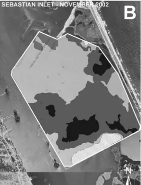
(4) collected on March 18th 2003 along two survey lines in the Indian River Lagoon southwest of the Sebastian Inlet entrance channel. RESULTS Classification of field data Two preliminary test surveys were conducted along the same planned survey lines on 50 kHz and 200 kHz signal frequency. Each dataset was split into four clusters, corresponding to the four known substratum classes (sea grass, dense algae, sparse algae, bare substratum) that occurred in the survey area (Figs. 2, 3). The classified, georeferenced signal locations were then resampled to a regular grid and classes were extrapolated to fill the blank spaces between the survey lines using a nearest-neighbor algorithm. The 200 kHz survey provided finer resolution (Fig. 2). While both surveys fairly accurately showed the shallow seagrass, the 200 kHz survey provided more detail with respect to the distribution of algae in the deeper (>1.5 m) water. This can probably be attributed to the. Fig. 2. Outcome of extrapolation of classes between testsurvey lines on (a) 50 kHz (b) 200 kHz in the Sebastian River study area. The smaller footprint of the 200 kHz transducer provides a finer-grain survey and therefore less confusions between sparse algae and bare substratum. Black=dense algae, grey=sparse algae, striped=seagrass. The groundtruthing concentrated on the shallow areas around the seagrasses, therefore accuracies in Table 1 are comparable between the two surveys. More grountruthing points in the algae area (lower part of the surveys) would have increased the accuracy of the 200 kHz survey favorably.. 168. Fig. 3. Survey results near Sebastian Inlet on 50 kHz. Black=dense algae, medium grey=sparse algae, light grey=bare seafloor, striped=seagrass. Groundtruthing locations for the calculation of confusion matrices in Table 1 are indicated as black circles.. smaller footprint of the 200 kHz signal. The bigger 50 kHz footprint would have picked up more algae signal in areas of very sparse algae, where the much smaller 200 kHz footprints would have missed the individual algae clumps and recorded bare substratum. This may explain the rather large disparity between the areas mapped as containing sparse algae in the two surveys (Fig. 2). Over a larger survey area and with a coarser survey grid (wider line-spacing), the 50 kHz results (Fig. 3) resembled more the 200 kHz results, inasmuch as the area that was identified on the fine-grid survey as having much sparse algae cover did not show this on the extrapolated large-scale map. This demonstrates the influence exerted on the results by the spacing of survey lines. In this larger-scale survey, the seagrass area in the northeastern corner (upper left in Figs. 2 and 3) did not show, as it was subsummed into a polygon of sparse algae.. Rev. Biol. Trop. (Int. J. Trop. Biol. ISSN-0034-7744) Vol. 53 (Suppl. 1): 165-174, May 2005 (www.tropiweb.com).
(5) This was an artifact of the extrapolation, where the more frequent algae signals “drowned out” the sparser seagrass signals. Field calibration For the production of a calibration dataset that only included chosen, well controlled, bottom classes, the vessel was anchored at the bow and stern to avoid any movement. Data were only accepted if all georeferenced datapoints fell into a narrowly confined space (essentially almost a single point). In the case of a drifting boat, the navigation points show a line and calibration data were discarded since it could not be assured that calibration files only contained data from a single bottom type. One dataset targeted mainly seagrass and was taken depths of 0.3, 0.9, 1.2 and 1.3 m. It differentiated dense and sparse seagrass from bare substratum and algae (Fig. 4). Bare substratum and algae signals occurred within the same data sequence (Fig. 4 B), since a slight surge rolled the seagrass in and out of the transducer footprint. In a second trial, algae were successively added into the transducer’s footprint to contain the following categories: no algae, sparse algae (250 g m-2), dense algae (2000 g m-2). The classification returned three classes corresponding. to bare substratum, sparse algae and dense algae (Fig. 5). The dataset contained data from 1.2 m and 1.5 m depth. During cluster analysis, it was possible to split data into three classes that discriminated between the levels of the algae. A single distinct class only appeared when algae were added over the sand. Therefore, we are confident that this class represents the acoustic trace of the drift algae. The wave-forms illustrated in Fig. 5 from seafloor in 1.5 m depth with and without algae show differences in the peaks. Waveforms from the bare substratum having one clean peak, while apparently destructive interference caused the waveforms returned from the algae to have several peaks and a more complicated trailing-edge. Results were comparable for the 0.8 m, 1.2 m and 1.8 m datasets as well as for a pooled dataset. Laboratory calibration The analysis used a simulated seafloor (wire basket suspended in the water) with variable density of algae (2000 g m-2, 250 g m-2, no algae at all) anchored at 0.8 m, 1.3 m and 1.8 m underneath the transducer. In all cases a threeclass split was obtained of which at least one class could be assigned to dense algae. When. Fig. 4. Results of field calibration experiment to confirm that four seafloor classes that were expected to be seen indeed had separable acoustic signatures. (A) PCA of acoustic signals after assignment of clusters, which are color coded and separate well seagrass of different densities, algae and bare substratum. (B) Sequence of signals, color coded for cluster membership, on a bathymetry plot. Algae, sparse seagrass and dense seagrass are well separated. The algae and bare substratum signals occur in mixed sequence, since a slight surge rolled algae in and out of the transducer footprint. The signal is scattered at a lower depth when algae are present, which helps to confirm the interpretation of the cluster analysis.. Rev. Biol. Trop. (Int. J. Trop. Biol. ISSN-0034-7744) Vol. 53 (Suppl. 1): 165-174, May 2005 (www.tropiweb.com). 169.
(6) Fig. 5. Field calibration to confirm that algae indeed have a clear acoustic signature. (A) PCA and subsequent cluster assignment (B) Sequence of signal. Algae were sequentially (first sparse, then dense) introduced into the footprint after a sequence of bare substratum signals was collected. Thus, the latter part of three sequences show increasing amounts of algae signals (grey=sparse algae and black=dense algae).. the datasets with only the sparse algae and the empty basket and then only the dense algae and the empty basket were merged, results were not clear for the sparse algae which did not always separate clearly from the emptybasket signals. When dense algae were added and data were split into two clusters, a clear split of the groupings was achieved indicating that an algae signal could be detected (Fig. 6). The analysis with the basket anchored at 0.8 m gave the clearest results and the signal was indeed capable of recognizing differences between dense algae, sparse algae and the seafloor. Three clusters (dense algae, sparse algae, bare basket) were observed. It was also clearly evident that the empty basket alone did not cause enough scatter to form its own signal cluster or to confuse the algal signal, since a sudden increase in measured depth once the algae were removed showed that the empty basket was not detected acoustically at all. This suggests sufficient scattering capability of even individual clumps of algae at shallow depth and discounts the possibility that the basket could have caused a scatter that could have been misinterpreted as algae-scatter. Groundtruthing results Review of the video surveys revealed the presence of the same four bottom types 170. predicted by the acoustic field survey (bare substratum; sparse algae; dense algae; seagrass). The groundtruthing only encompassed three of the four bottom type categories since no areas of dense algae was encountered within the survey track. Therefore results for this area are based on merging the dense and sparse algae classes of the groundtruthing survey into one ‘algae’ class. Two confusion matrices were produced which compared the spatial prediction models derived from the 50 kHz survey and that from the 200 kHz survey. Overall, the predicted classification based on the acoustic data performed reasonably well on both frequencies, with an overall accuracy of about 60% (Table 1). The surveys and resulting spatial prediction models (maps) were very good at predicting areas of algae (96 and 97%), however some confusion did exist between areas of sand and seagrass. This result suggests that both signal frequencies have a comparable ability of differentiating between the three bottom classes. DISCUSSION The results from above analyses suggest that acoustic seafloor discrimination is not only able to tell different sediment types from each other (Hamilton et al. 1999, Morrison et al. 2001) but that it is also capable of. Rev. Biol. Trop. (Int. J. Trop. Biol. ISSN-0034-7744) Vol. 53 (Suppl. 1): 165-174, May 2005 (www.tropiweb.com).
(7) Fig. 6. Laboratory calibration to confirm field results: three-cluster split in a calibration dataset that contains the empty basket, dense algae and sparse algae in between. (A) PCA of acoustic signals after assignment of clusters, which are color coded. (B) Sequence of signals, color coded for cluster membership, on a bathymetry plot. Dense algae, sparse algae and empty substratum (the basket does not show up at all) are well separated. Algae clearly produce an acoustic signal, since both dense and sparse algae reflect the signal at the height of the basket (0.7 m). When algae were removed, the signal was not scattered on the empty basket, but only on the underlying seafloor at 1.6 m depth. TABLE 1 Class-by-class error matrix for the extrapolated maps developed for the Sebastian Inlet study area. Video Surveys. A.. sand seagrass algae Total # of points: Accuracy (%). sand. Sebastian Inlet 50 kHz seagrass. algae. 14 12 4. 66 28 16. 1 2 115. Overall:. 30 46.67. 110 25.45. 118 97.46. 258 60.85. B. Video Surveys. sand. Sebastian Inlet 200 kHz seagrass algae. User accuracy%. sand seagrass algae. 0 5 4. 17 41 0. 13 64 114. 0 37.3% 96.6%:. Total # of points: Producer Accuracy (%). 9 0. 58 71%. 191 59.7%. 258 60.1%. Accuracy is indicated for individual classes as well as overall performance of the model. (A) 50 kHz survey (B) 200 kHz survey.. Rev. Biol. Trop. (Int. J. Trop. Biol. ISSN-0034-7744) Vol. 53 (Suppl. 1): 165-174, May 2005 (www.tropiweb.com). 171.
(8) detecting algae and seagrass. From both calibration experiments and field survey data it was apparent that seagrass and drift algae indeed produce unique echo classes both on 50 and 200 kHz frequency. However, both under laboratory conditions and in the field, it proved difficult to obtain files containing only echoes that could be clearly ascribed to either algae or seagrass. In all files that contained echoes from algae or seagrass, a large proportion of echoes (about half) clustered together with echoes obtained from bare substratum. This suggests that the bottom signal occurred as frequently as the algae and seagrass signals themselves. Seagrass had a more pronounced signal than algae and overall had less confusion with bare substratum. The reason for this confusion may either be a relatively weak scattering ability of the algae and seagrass or could be found in the signal processing properties. QTC View takes the entire signal envelope of the first echo (it ignores multipath echoes) into account (Collins et al. 1996, Collins and Lacroix 1997) and this was found by Preston et al. (2000) to provide good discrimination ability of sediment geotechnical variables. According to Chivers et al. (1990), the first peak(s) of the echo is strongly influenced by subsurface reverberation, while the echo’s tail primarily encodes scatter. Since. Fig. 7. Comparison of waveform returns from bare sand and dense algae (echoes of 50 kHz signal).. 172. the algae form only a loose mass above the substratum, it can be expected that enough acoustic energy can traverse the algae layer to interact with the substratum. Also, the strength of the algae’s interference with the sound waves may depend on their orientation, which constantly changes while clumps of algae are rolled by even the slightest surge in the shallow water. Depending on orientation, the algae may therefore appear more or less dense to the signal, resulting in differential modification of the first peak or they may act primarily to scatter and modify the tail of the signal (Fig. 7). Therefore, the substratum on which the algae are placed will play an important role in the overall shape of the signal, even if this should carry algae or seagrass information. In practice this means that the production of a calibrated “signal library”, which can later be used for supervised classification of survey data (Anonymous 2000) is difficult. Unless the signal library contains algae/no algae, seagrass/ no seagrass pairs for exactly the same sediment classes as found in the survey area, it is likely that confusion is introduced. Since the exact distribution of sediment classes in the survey areas was unknown, we were not able to build a full suite of calibration files useful for supervised classification of surveys over unknown bottom classes. It was interesting to note that the signal frequency did not have a clear influence on discrimination accuracy, although the shorter 200 kHz signal should scatter on smaller particles (Preston et al. 2000) and might therefore have been expected to scatter more easily on aquatic flora. Overall, the survey results obtained with the 200 kHz frequency were, however, found to be preferable because the footprint (insonified seafloor area) of the 200 kHz transducer was less than one quarter the size of that of the 50 kHz transducer. This allowed to decrease the size of the sampled seafloor in each series of four stacked echoes that form the final sampling unit, which leads to increased “sharpness” of detected spatial patterns (Fig. 2). In conclusion, we find that acoustic seafloor discrimination is a viable way of mapping. Rev. Biol. Trop. (Int. J. Trop. Biol. ISSN-0034-7744) Vol. 53 (Suppl. 1): 165-174, May 2005 (www.tropiweb.com).
(9) the patterns of distribution in benthic flora in a shallow, turbid lagoonal setting of mostly less than 2 m water depth. The 60% accuracy of a low-order discrimination (sand-seagrassalgae) was found acceptable. It is believed that further research could increase the accuracy of discrimination into more classes. Where optical remote sensing cannot be used for the description of large-scale patterns of aquatic flora, acoustic ground discrimination appears to be the next best option in terms of cost-efficiency and accuracy. ACKNOWLEDGMENTS This study was funded by the St. Johns River Water Management District under contract SF655AA. BR and RPM were also supported by NOAA grants NA16OA1443 and NA03NOS4260046 to NCRI. This is NCRI publication Nº 51. RESUMEN La distribución espacial de comunidades de pastos marinos y algas puede ser difícil de determinar en sistema lagunares grandes y someros donde la alta turbidez no permite el uso de métodos ópticos, como fotografías aéreas e imágenes satelitales. Complicaciones adicionales pueden surgir cuando las algas no están adheridas permanentemente al sustrato y derivan con las mareas y corrientes. Se realizó un estudio utilizando discriminación acústica del fondo marino en el Indian River Lagoon (Florida, EUA) para determinar la cantidad de algas y pastos que derivan. Se realizaron sondeos acústicos en el Sebastian Inlet con el sistema QTC View V y transductores de 50 y 200 kHz. Las áreas de pastos marinos pudieron ser identificadas, y están mezcladas con una gran cantidad de algas a la deriva. Se rellenó los espacios sin datos con extrapolaciones basadas en la técnica del “vecino más cercano”, produciendo un mapa espacialmente coherente. Comprobaciones de campo con video y “matrices de confusión” indican que los mapas tienen un alto nivel de concordancia (60%) con la distribución real de las algas; sin embargo, hubo cierta confusión entre arena y algas, y entre arena y pastos marinos. Palabras clave: Discriminación acústica del fondo, sensores remotos, pastos marinos, algas a la deriva, Laguna Río Indio, Florida.. REFERENCES Anonymous. 2000. QTC Impact User Manual. Quester Tangent Corporation, Canada. 110 p. Bates, C.R. & E.J. Whitehead. 2001. Echoplus measurements in Hopavagen Bay, Norway. Sea Technol. 42: 34-43. Chivers, R.C., N. Emerson & D.R. Burns. 1990. New acoustic processing for underway surveying. Hydrographic J. 56: 9-19. Collins, W.T. & P. Lacroix. 1997. Operational philosophy of acoustic waveform data processing for seabed classification. COSU 97, Oceanology International, Singapore 97: 225-234. Collins, W.T., R. Gregory & J. Anderson. 1996. A digital approach to seabed classification. Sea Technol. 37: 83-87. Green, E.P., P.J. Mumby, A.J. Edwards & C.D. Clark. 2000. Remote sensing handbook for tropical coastal management. Coastal Management Sourcebooks 3, UNESCO Paris. 316 p. Hamilton, L.J. 2001. Acoustic seabed classification systems. Department of Defence, Defence Science and Technology Organization (Australia). 150 p. Hamilton, L.J., P.J. Mulhearn & R. Poeckert. 1999. Comparison of RoxAnn and QTC-View acoustic bottom classification system performance for the Cairns area, Great Barrier Reef, Australia. Cont. Shelf Res. 19: 1577-1597. Lawrence, M.J. & C.R. Bates. 2001. Acoustic ground discrimination techniques for submerged archaeological site investigations. MTS Journal 35: 65-73. Legendre, P. 2002. Acoustic seabed classification methodology: a user’s statistical comparison. Departement de Sciences Biologiques, Universite de Montreal. 17 p. Legendre, P., K.E. Ellingsen, E. Bjornbom & P. Casgrain. 2002. Acoustic seabed classification: improved statistical methods. Can. J. Fish. Aquat. Sci. 59: 1085-1089. Morris, L.J. & L.M. Hall. 2001. Estimating drift algae abundance in the Indian River Lagoon, FL. St. Johns River Water Management District Tech. Memo. 10 p. Morris, L.J., R.W. Virnstein, J.D. Miller & L.M. Hall. 2000. Monitoring changes in Indian River Lagoon, Florida, using fixed transects, p. 167-176. In S.A. Bortone (ed.). Seagrass Monitoring, Ecology, Physiology and Management. CRC Press, Boca Raton.. Rev. Biol. Trop. (Int. J. Trop. Biol. ISSN-0034-7744) Vol. 53 (Suppl. 1): 165-174, May 2005 (www.tropiweb.com). 173.
(10) Morrison, M.A., S.F. Thrush & R. Budd. 2001. Detection of acoustic class boundaries in soft sediment systems using the seafloor acoustic discrimination system QTC VIEW. J. Sea Res. 46: 233-243. Mumby, P.J. & E.P. Green. 2000. Field survey: building the link between image and reality, p. 57-67. In E.P. Green, P.J. Mumby, A.J. Edwards & C.D. Clark (eds.). Remote Sensing Handbook for Tropical Coastal Management. Coastal Management Sourcebooks 3, UNESCO, Paris. Prager, B.T., D.A. Caughey & R.H. Poeckert. 1995. Bottom classification: operational results from QTC View. Oceans ’95, San Diego, October 1995. Pp. 1827-1835. Preston, J.M., A. Rosenberger & W.T. Collins. 2000. Bottom classification in very shallow water. Proc. Oceans 2000, Newport. Pp. 1563-1567. Preston, J.M., W.T. Collins, D.C. Mosher, R.H. Poeckert & R.H. Kuwahara. 1999. The strength of correla-. 174. tions between geotechnical variables and acoustic classifications. Proc. MTS/IEEE OCEANS’99 Conf., September 1999. Pp. 1123-1128. Preston, J.M., A. Rosenberger, & W.T. Collins. 2000. Bottom classification in very shallow water. Proc. Oceans 2000, Newport: Preston, J.M., A.C. Christney, L.S. Beran, W.T. Collins & R.A. McConnaughey. 2002. Objective measures of acoustic diversity for benthic habitat characterization. Symp. Effects Fisheries Benthic Habitats: Linking Geology, Biology, Socioeconomy and Management, Tampa 2002. Pp. 45. Virnstein, R.W. & P.A. Carbonara. 1985. Seasonal abundance and distribution of drift algae and seagrass in the mid-Indian River Lagoon, FL. Aquat. Bot. 23: 67-82. Virnstein, R.W. & R.K. Howard. 1987. Motile epifauna of marine macrophytes in the Indian River Lagoon, Florida. II. Comparison between drift macroalgae and three species of seagrass. Bull. Mar. Sci. 41: 13-26.. Rev. Biol. Trop. (Int. J. Trop. Biol. ISSN-0034-7744) Vol. 53 (Suppl. 1): 165-174, May 2005 (www.tropiweb.com).
(11)
Figure


+3


Documento similar
In the “big picture” perspective of the recent years that we have described in Brazil, Spain, Portugal and Puerto Rico there are some similarities and important differences,
In addition, precise distance determinations to Local Group galaxies enable the calibration of cosmological distance determination methods, such as supernovae,
Government policy varies between nations and this guidance sets out the need for balanced decision-making about ways of working, and the ongoing safety considerations
No obstante, como esta enfermedad afecta a cada persona de manera diferente, no todas las opciones de cuidado y tratamiento pueden ser apropiadas para cada individuo.. La forma
Keywords: iPSCs; induced pluripotent stem cells; clinics; clinical trial; drug screening; personalized medicine; regenerative medicine.. The Evolution of
Astrometric and photometric star cata- logues derived from the ESA HIPPARCOS Space Astrometry Mission.
The photometry of the 236 238 objects detected in the reference images was grouped into the reference catalog (Table 3) 5 , which contains the object identifier, the right
In the empirical models, the isotherms were divided in two parts (from 0.11 to 0.57 and brom 0.75 to 0.94), and the data obtained at a water activity level of 0.70 has not been
