Segmentación de imágenes de resonancia magnética para generar superficies de piel

Instituto Tecnol ´ogico de Costa Rica

Escuela de Ingenier´ıa en Electr ´onica

Segmentaci ´on de im´agenes de resonancia magn´etica para generar superficies de piel (Segmentation of MR images for skin surface model generation)

Informe de Proyecto de Graduaci ´on para optar por el t´ıtulo de Ingeniero en Electr ´onica con el grado acad´emico de Licenciatura

Alexander Singh Alvarado

Declaro que el presente Proyecto de Graduaci ´on ha sido realizado por mi persona, utilizando y aplicando literatura referente al tema, as´ı como la informaci ´on que haya suministrado la empresa para la que se realizar´a el proyecto, y aplicando e intro-duciendo conocimientos propios.

En los casos en que he utilizado bibliograf´ıa, he procedido a indicar las fuentes mediante las respectivas citas bibliogr´aficas.

En consecuencia, asumo la responsabilidad total por el trabajo de graduaci ´on realiza-do y por el contenirealiza-do del correspondiente informe final.

Resumen

Los m´etodos actuales en cirug´ıa guiada por im´agenes incluyen el aro estereot´axico y sistemas ´opticos que han sido dise ˜nados para mapear la informaci ´on obtenida de las im´agenes y planeamientos quir ´urgicos hacia la anatom´ıa del paciente.

Actualmente en el laboratorio de radio cirug´ıa/biolog´ıa del Instituto McKnight Brain se est´a trabajando en el dise ˜no de un nuevo sistema de cirug´ıa estereot´axica. Este se utilizar´a para crear prototipos de m´ascaras hechas a la medida del paciente.

Para el desarrollo de estas m´ascaras se requiere una representaci ´on confiable de la superficie de la piel. El molde o m´ascara ser´a dise ˜nado bas´andose en ´esta superficie generada a partir de la segmentaci ´on de im´agenes obtenidas por MRI (im´agenes de resonancia magn´etica).

Este tipo de im´agenes presentan varios problemas. Estos incluyen inhomogeinidades en la intensidad a trav´es de los cortes axiales y una relaci ´on se ˜nal a ruido baja. Debido a estos problemas la detecci ´on de los bordes basado solamente en el nivel de grises lleva a resultados incorrectos en la identificaci ´on de la superfice de la piel y por ende en el dise ˜no de la m´ascara.

El prop ´osito de este proyecto es la implementaci ´on de un algoritmo de segmentaci ´on para un conjunto completo de im´agenes MRI que identifique el borde de la piel con una precisi ´on de±2mm y en menos de 5 minutos. Bajo ´estas condiciones una m´ascara de dimensiones confiables puede ser dise ˜nada.

En el campo de im´agenes m´edicas varias t´ecnicas de segmentaci ´on pueden ser apli-cadas incluyendo: region growing, watersheds, level set y active contours. Debido a las caracter´ısticas de las MRI los ASM (active shape models) han sido elegidos. Los ASM se basan en un conjunto de im´agenes de entrenamiento. De ´estas imagenes se captura la variabilidad en las formas. El modelo generado junto con el m´etodo de deformaci ´on constituyen un algoritmo robusto y eficiente para la detecci ´on de contornos.

Palabras claves:

ABSTRACT

Current methods in image guided surgery include the stereotactic head ring and optical systems which have been designed to map the information obtained from images and surgery planning on to the patients anatomy.

The radio surgery/biology laboratory at the McKnight Brain Institute is currently working on a system to design and create rapid prototyping models for image guided surgery which have economical and functional advantages over currently used meth-ods.

In order to create these models a 3D representation of the human skin surface is necessary. The fixture or model will be designed based on this surface, which can be derived from segmenting an MRI (Magnetic Resonance Image) data set.

MR images present various problems, including intensity inhomogeneities along the slices and a low signal to noise ratio. These are a consequence of technical aspects in the image reconstruction. Because of these problems segmentation based on thresh-olding does not lead to a correct identification of the skin border.

The purpose of this project which extends from the rapid prototyping system is toward the design and implementation of a segmentation algorithm that will identify the skin border with a precision of± 2mm and in less than 5 minutes for every data set. Under these conditions a reliable fixture can be designed in the aid of stereotactic surgery.

In medical imaging various segmentation techniques are employed, including region growing, watersheds, level set and active contours. Because of the MR image char-acteristics the active shape model approach has been selected. Combining shape restrictions and image-based information for border detection.

Key words:

Acknowledgments

I would like to thank Dr. Frank Bova for his trust and for the opportunity to work at the radio surgery/Biology laboratory.

To my new friends Dr. Didier Rajon, B´arbara Garita and Atchar Sudhyadhom for their advice and help during the preparation of this thesis. I would specially like to thank my adviser Dr.-Ing. Jos´e Pablo Alvarado Moya, who inspired my curiosity into image processing and helped me with my first steps.

Finally I’d like to thank my dear friends Suresh, Eric, Samir and Carlos, and my family for their support during the project.

Contents

1 INTRODUCTION 1

1.1 Problem statement . . . 1

1.1.1 Problem Context . . . 1

1.1.2 Problem Definition . . . 3

1.2 Solution Proposed . . . 4

1.3 Structure of this work . . . 5

2 GOAL & OBJECTIVES 7 2.1 Goal . . . 7

2.2 General Objective . . . 7

2.3 Specific Objectives . . . 7

3 THEORETICAL FRAMEWORK 9 3.1 Research area description . . . 9

3.1.1 NMR (Nuclear Magnetic Resonance) . . . 9

3.1.2 MRI (Magnetic Resonance Image) . . . 18

3.2 Current project state . . . 21

3.2.1 Fixtures . . . 22

3.3 Image domain segmentation techniques used in medical MRIs. . . 24

3.3.1 Region growing . . . 25

6.2.1 Over the AC-PC plane: Top of the head . . . 59

6.2.2 Under the AC-PC plane: nose curvature . . . 60

6.3 Comparison obtained using thresholding and ASM . . . 60

6.3.1 Over the AC-PC plane: Top of the head . . . 61

6.3.2 Near AC-PC plane . . . 62

6.3.3 Under the AC-PC plane: nose curvature . . . 62

6.4 3D model generation . . . 64

6.5 Processing Time . . . 66

6.6 Future work . . . 66

6.6.1 False edge detection . . . 66

6.6.2 Pre-processing . . . 67

6.6.3 Shape variation in young patients . . . 67

6.6.4 Automatic landmark placement . . . 68

7 CONCLUSIONS AND RECOMMENDATIONS 69 7.1 Conclusions . . . 69

7.2 Recommendations . . . 70

A Glossary 73

B McKNight Brain Institute description 75

List of Figures

1.1 Magnetic Resonance Image (left). Close up at pixel level (right) . . . . 4

1.2 MR images taken at different depths in the human head. . . 4

1.3 Block diagram for the general solution. . . 5

3.1 Magnetic field induced by the spin in the proton [2]. . . 10

3.2 Magnetic field effect over proton alignment [2]. . . 11

3.3 Precession effect over the proton in the presence of a magnetic field [2]. 12 3.4 The magnetization vector and its components. . . 12

3.5 T2, free induction decay time. . . 13

3.6 T1, return to equilibrium time. . . 14

3.7 Generation of the gradient field. . . 16

3.8 Gradient field applied to the patients body. . . 17

3.9 The inclination of the gradient affects the slice thickness. . . 17

3.10 Example of an MRI machine designed specially for patients that suffer from claustrophobia [17] . . . 18

3.11 Example of a MRI image taken from a set with a resolution of 512 x 512 x 119. . . 19

3.12 The different views of the human anatomy used to analyze CT and MRIs.[14] . . . 20

3.13 Examples of a CT (left) and MRI (right) scans. . . 21

3.14 Patient with a head ring [13] . . . 21

3.16 Fixture created based on a head model. . . 22

3.17 Fixture created using 3D printer with the guide to hold the probe. . . 23

3.18 Example of the fixture use. . . 23

3.19 Zprinter 310 three dimensional printer used to create the fixtures. . . . 24

3.20 Zprinter 310 printing process. . . 24

3.21 Watershed algorithms based on immersion (left) and rain-fall (right). . 25

3.22 Example of how the snake adapts to the specific regions. . . 26

4.1 Scheme for the evaluation of the segmentation algorithms . . . 28

5.1 Marr-Palmer’s computational vision framework for human perception. 31 5.2 Example of an MRI scan. . . 33

5.3 Examples of two MR images taken from different scanners. . . 33

5.4 Partial volume effect. . . 34

5.5 The inverse Fourier transform will cause bottom slices to reappear on the top slices. . . 35

5.6 Block diagram for the general solution. . . 37

5.7 Illustration of the eigenvectors for a set of 3D points. . . 39

5.8 Effect of varying the elements in the B vector. The shapes have been scaled and translated in order to be displayed. . . 42

5.9 Landmark assignment near the tip of the nose. . . 43

5.10 Distribution of the patients by age at treatment in the radiosurgery database at the McKnight Brain Institute. . . 44

5.11 Point based displacements. . . 45

5.12 Gray level profile creation based on adjacent points. . . 46

5.13 Profile scanning. . . 47

5.14 The suggested shape in red and the shape when the constraints are applied in blue. Figures 1a and 2a show this process at the nose level. Figures 1b and 2b are near the AC-PC plane. . . 47

5.16 Intermediate tests applied to the ASM during the implementation. The test image was transformed by adding noise, warping and smoothing. 49

5.17 Setup in the MR scanning room.[8] . . . 50

5.18 The patients head can be tilted as seen in the sagittal view (lower left). 51 5.19 3-D dataset interpreted in a world coordinate system. . . 52

5.20 Location of the anatomical landmarks. [6] . . . 52

5.21 Identification of the landmarks. . . 53

5.22 Coordinate system defined by the anatomical landmarks. . . 54

5.23 Coordinate transformation. . . 55

6.7 Superposition of the mask generated by the ASM and thresholding over the CT reference for a slice near the top of the head. Blue: CT reference. Red: mask generated by thresholding. Green: mask generated by the ASM. . . 61

6.8 Superposition of the mask generated by the ASM and thresholding over the CT reference for a slice above the AC-PC plane. Blue: CT reference. Red: mask generated by thresholding. Green: mask generated by the ASM. . . 62

6.9 Superposition of the mask generated by the ASM and thresholding over the CT reference for a slice at the nose level. Blue: CT reference. Red: mask generated by thresholding. Green: mask generated by the ASM. . . 62

6.12 Surface generated by the ASM. . . 65 6.13 Qualitative comparison between the ASM results and thresholding

List of Tables

3.1 Magnetic resonance properties of medically useful nuclei [2]. . . 10 3.2 Gyromagnetic ratio for useful elements in magnetic resonance [2]. . . . 12 3.3 T1 and T2 relaxation constants for several tissues [2] . . . 15 6.1 Sum of the square of the border differences between the segmentation

Chapter 1

INTRODUCTION

1.1

Problem statement

1.1.1

Problem Context

The radio surgery and radio biology laboratory at the McKnight brain institute is currently developing a system to design and create rapid prototyping models for image guided surgery. The following description is based on the grant proposal NIH-NIBIB Grant # 5R01EB2573-3 [13].

The next generation of surgical planning applies the optimized virtual plans at the time of surgery. This is possible by evaluating alternate surgical approaches through the manipulation of the patients specific virtual 3D data set. The ability to apply the virtual surgical plan to the real world patient at the time of surgery is termed image guided surgery.

Image guided surgery is divided in two categories, frameless and frame based.

Frame based stereotactic surgery

In frame based stereotactic or image guided surgery the reference frame will incor-porate necessary trajectories for guidance including mechanical referencing to the patient at the time of surgery, guidance for initial skin incision, position and design of the required craniotomy, trajectory alignment to the large tissues and a mechanical platform used to mount other surgical tools such as retractors or skin clips.

• Bulky obtrusive equipment.

• Technical difficulties tracking surgical instruments.

• The requirements for special scans and special training.

• Cost of replacement parts.

• Because of the pain involved in frame placement pediatric patients must un-dergo general anesthesia prior to frame application.

The apparatus used during diagnostic imaging contains reference fiducials that are embedded in each diagnostic image. These fiducials provide means to map the image back to the stereotactic frame’s coordinate system see Figure 3.14.

Frameless stereotactic surgery

Fiducial landmarks are derived from the patients own anatomical features [11]. These fiducial replace the frame based fiducials.

Rigid frame based systems such as those used in stereotactic biopsy and radiosurgery have an advantage in their rigidity and in their ability to eliminate the geometry errors.

For frame less patients the time sequence is somewhat more relaxed. When external fiducials are required, they can be applied to the patient the day prior to surgery. When using frameless systems the shift of skin must be contemplated. For example if the medial canthus and lateral canthus are to be used as anatomic landmarks, selecting their exact position in the 3 dimensional reconstructing of the diagnostic datasheet can be influenced by:

• Type dataset CT/MR.

• Patient eyes are open continually blinking during the scan or if their eyes are closed and if so how tight.

At the radio surgery/biology laboratory an innovative model based guidance system is being developed. The aim of the rapid prototyping tool is to develop a new class of biopsy tool an operative instrument for specific individual patient needs and linked to the patients unique construct. Time from scanning to procedure is measured in hours and not days or weeks.

This system avoids the requirements of special equipment to be present within the operating room and the guide can be applied and removed as needed.

If successful it could be applied to all cranial procedures and would result in great improvement in the accuracy of shunt placement, skin incision placement and bone flap placement making cranial neurosurgery accurate and minimally invasive. The estimated cost of materials per case is approximately $10.

The research done in the Radio surgery and Radio Biology laboratory at the McKnight brain institute is toward the design of new fixtures for guided surgery based on MRI or CT scans that in some cases will fulfill the same task as the stereotactic frame. The overall accuracy goal for these fixtures lies within ± 2mm.

At this moment the system under development presents an inaccurate reconstruction of the three dimensional model based on the MRI, therefore the fixtures which are designed in accordance to this model are not reliable. The segmentation algorithm being used to determine the head contour is based on a Gaussian filter and gray level threshold.

1.1.2

Problem Definition

Magnetic resonance images present various problems that make segmentation a dif-ficult task. Figure 1.1: shows a typical MR image in which the following problems can be identified:

• Low signal to noise ratio.

• Intensity inhomogeneities.

• Low contrast between the skin surface gray level and the air immediately outside the patients contour.

The image quality is a reflexion of the technical limitations in MRI scanning. These characteristics can lead to segmentation errors such as false edge detection, over tessellation and gaps in borders and edges.

Figure 1.1: Magnetic Resonance Image (left). Close up at pixel level (right)

Figure 1.2: MR images taken at different depths in the human head.

If a slice is taken close to the top of the head the contour will resemble that of an oval. As the depth progresses, the eyes, ears and nose appear changing the boundary. Because of the shading effect the gray levels at the edges will also vary depending on the depth.

The problem lies in the difficulty of processing the images due to the quality of MR scans and the variation of the head contour.

1.2

Solution Proposed

variations of each type. The selection of an appropriate technique for a specific type of image is a difficult problem [15].

There are several factors that make it difficult to choose a segmentation algorithm, because there is no common ground from which it is possible to compare the results of each algorithm.

In order to quantify the performace of a segmentation method validation experiments are necessary [21]. However there’s a difficulty in implementing other people’s al-gorithms due to the lack of necessary details [20]. The alal-gorithms have also been designed for an specific type of image and a specific application.

By carefully analyzing the problems present in MR imaging the algorithm that best fits this task is the active shape model. But in order to make use of this segmentation technique pre-processing modules are required such as those shown in Figure 1.3.

Original 3-D

Figure 1.3: Block diagram for the general solution.

In order to validate the implementation of the algorithm empirical discrepancy [22] methods will be applied with a fused set of CT and MR images.

The CT images have a higher spatial resolution therefore the contours can be easily determined using simple segmentation algorithms. These contours can then be used as the ground truth for the evaluation function, of the segmented MR images.

1.3

Structure of this work

Chapter 4 refers to the solution itself, and justifies the selection of the ASM as the seg-mentation algorithm followed by a detailed description of the mathematical concepts explaining ASM.

Chapter 5 shows the results obtained from using the ASM in the segmentation of MR images and the comparison with the results obtained from the current thresholding methods.

Chapter 2

GOAL & OBJECTIVES

2.1

Goal

• To develop reliable fixtures and guides to be used in neurological surgery.

2.2

General Objective

• Develop a segmentation algorithm to identify a patients head contour in axial T1 MRIs

2.3

Specific Objectives

• Develop and implement a head contour detection software compatible with the rapid-prototyping system at the McKnight Brain Institute.

• Implement discrepancy evaluation methods to assess the segmentation algo-rithm.

Chapter 3

THEORETICAL FRAMEWORK

3.1

Research area description

In order to understand completely the problem and the solution, certain concepts must be established.

3.1.1

NMR (Nuclear Magnetic Resonance)

The following subsection on nuclear magnetic resonance is based on [2].

Magnetic resonance imaging is based on nuclear magnetic resonance (NMR). The NMR phenomenon relies on the fundamental property that protons and neutrons that make up a nucleus possess an intrinsic angular momentum called spin [12]. The proton is a charged particle with a nuclear spin that produces a magnetic dipole. An analogy can be made considering a spiral with a direct current as seen in figure 3.1. The direction of the current will define the polarity of the magnetic field.

The neutron on the other hand does not present a charge but it does have a magnetic field opposite and approximately of the same magnitude as the protons which is caused by charge inhomogeneities at sub nuclear scale.

Protons have a magnetic field that is created by this rotation. When protons and neutrons combine to form nucleus, they combine with oppositely oriented spins [12], therefore if the number of protons and neutrons in the nucleus are equal the overall magnetic field is zero. Elements constituted by an odd sum of protons and neutrons will present an net magnetic field.

pro-ducing MR images [2]. From table 3.1 it can be seen that hydrogen has the highest magnetic moment and greatest abundance which makes it by far the best element for general clinical utility.

Charge differential Magnetic Field

Figure 3.1: Magnetic field induced by the spin in the proton [2].

Table 3.1: Magnetic resonance properties of medically useful nuclei [2]. Nucleus Spin

state protons are found in a ratio of 3 per million under a 1.0T field considering that a typical voxel volume in MRI contains about 1021 _{protons, there are 3·10}15 _more spins in the low energy state [2].

Parallel

Anti-Parallel Magnetic

Field

Figure 3.2: Magnetic field effect over proton alignment [2].

Another important characteristic of protons is that they also experience a torque force from the applied field that causes precession similar to how a spinning top wobbles due to the force of gravity. The angular frequency of this precession is defined by the Larmor equation (see Figure 3.3).

ω =α·Bo (3.1)

Where α is the gyromagnetic ratio and Bo is magnetic field magnitude. Based on

this equation it is seen that the resonant frequency of the protons depends on the magnetic field the proton is subject to. Each element has a unique gyromagnetic constant which allows for discrimination. Table 3.2 lists the gyromagnetic constants of elements useful in magnetic resonance [2].

The net magnetization vector M is described by three components (Figure 3.4). Mz

(longitudinal magnetization) is the component parallel to the applied field. At equilib-rium the longitudinal magnetization is maximum and is denotedMo. The amplitude

ofMz is determined by the excess number of protons that are in the low energy state. Mxy is the component perpendicular to the applied magnetic field and is also known

Larmor Frequency w

Figure 3.3: Precession effect over the proton in the presence of a magnetic field [2].

Table 3.2: Gyromagnetic ratio for useful elements in magnetic resonance [2]. Nucleus α [MHz/T]

1H 42.58

13C 10.7

17O 5.8

19F 40.0

23Na 11.6

31P 17.2

X

Y Z

Magnetization vector

M

Mxy

Component Mz

Component

When a radiofrequency signal is synchronized to the Larmor frequency of the protons the magnetic component of the RF wave will cause the protons that are aligned antiparallel to shift into alignment with the main magnetic field by absorbing energy. Once the RF signal is removed these protons will return to their original orientation by liberating energy. The return speed depends on the type of tissue.

The amplitude and duration of the RF pulse determines the overall energy absorption, if the application of the RF signal is continued it will induce the return to equilibrium conditions.

Free induction decay: T2

The RF pulse is applied during the necessary time for theM vector to have only one component which is transverse. Therefore once the RF signal is removed initially the

Mxy component is maximum and a decay in the amplitude of this component begins.

The decrease in the transverse vector is expressed by the equation which can also be seen in figure 3.5.

Mxy(t) = Moe−t/T2 (3.2)

where T2 is known as the decay constant and is the elapsed time between the maxi-mum magnitude and 37% of the peak level. The value of T2 can be used to determine the tissue type for example in non moving structures with stationary magnetic inho-mogeneities have very short T2 times.

1

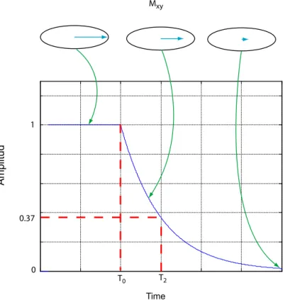
Return to equilibrium: T1

When the RF pulse is removed the Mz component starts to increase from 0 to Mo as

seen in Figure 3.6. This increment is expressed by the equation:

Mz(t) = Mo−Mo·e−t/T1 (3.3)

The T1 decay time occurs relatively quickly where as the return of the excited mag-netization to equilibrium takes longer. In this case T1 is the relaxation constant and is the time needed to recover the 63% of the longitudinal magnetization.

1

0 0.37

T2

T0

Mxy

Amplitud

Time

Figure 3.6: T1, return to equilibrium time.

Based on the amplitude changes that can be registered by the receiver coils T1 and T2 can be estimated in order to identify the tissue. Table 3.3 shows T1 and T2 relaxation times for several tissues.

Table 3.3: T1 and T2 relaxation constants for several tissues [2] Tissue T1 0.5T (msec) T1 1.5T (msec) T2 (msec)

Fat 210 260 80

Liver 350 500 40

Muscle 550 870 45

White matter 500 780 90

Gray matter 650 900 100

Cerebrospinal fluid 1800 2400 160

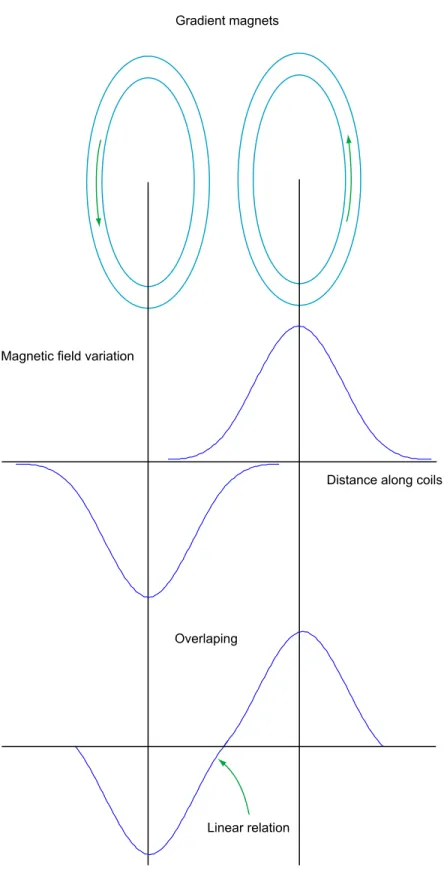
Gradient Magnets

Magnetic field gradients are obtained by super imposing the magnetic fields of one or more coils with a precisely defined geometry. With the appropriate design the gradient coils create a magnetic field that linearly varies in strength versus distance over a predefined field of view as seen in figure 3.7

By generating a linear dependent field vs distance as seen in figure 3.8 the Larmor frequency will also vary linearly, this can be used for slice selection.

Magnetic field variation

Distance along coils

Overlaping

Linear relation Gradient magnets

Excited slice of tissue

Slice select gradient

Gradient coils

Narrow Band RF

Figure 3.8: Gradient field applied to the patients body.

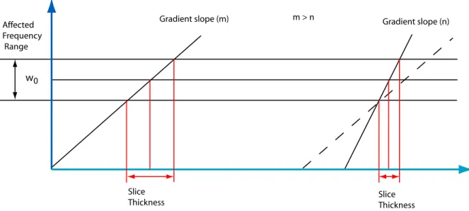
w₀

Affected Frequency Range

Slice

Thickness Slice _Thickness

Gradient slope (m) m > n _{Gradient slope (n)}

3.1.2

MRI (Magnetic Resonance Image)

To obtain a MRI the object is placed under a constant magnetic field. The intensity of this field varies depending on the MRI equipment (ranging from 0.1T to 4.0T [2]). Gradient magnets are used to alter the magnetic field in a specific region. This is only true for the section defined by the orientation of the gradient magnets. The position of these magnets can be used to select the orientation of the slice that will be taken from the object.

Once the area of interest has been chosen by aligning the gradient magnets, radio fre-quency pulses are emitted toward the region. Because the magnetic field is different in each region the Larmor frequency is also different. Therefore when the radio fre-quency pulses are emitted only the protons that are found inside the corresponding magnetic field will begin to resonate. When this occurs they increase their energy level by shifting toward an anti parallel position in relation to the main magnetic field. Once the radio frequency pulses are switched off the protons slowly return to their original position. While emitting energy these radio frequency signals are captured and used to determine the relaxation times, T1 and T2, which depend on the nature of the composition of the object scanned.

This technique is widely used in medical applications (Figure 3.10) because of its advantages over other imaging techniques. It is a non invasive procedure and no radiation must be submitted to the patient which is not the case for CT scans. The images obtained have a high contrast resolution, different types of tissue are easily identified which makes it a powerful instrument when identifying tumors or organ pathologies.

But there are also disadvantages:

• Patients that carry any metal objects inside their bodies might not be subject to a MRI scan

• Although the contrast resolution is very high the spatial resolution is poor. In some cases a contrast substance such as gadolinium may be used to enhance visibility of certain tissue or blood vessels.

Image Characteristics

The images obtained from a MRI scan have low quality, because of several factors [12]:

• inhomogeneity of the magnetic field.

• Radio frequency inhomogeneity can yield intensity variations in the order of 10-20%.

• Partial volume effect which occurs when multiple tissues are present in a voxel.

• Random Noise affects all MR images.

An example of a MRI image taken from a 3-D data set with a resolution of 512 pixels x 512 pixels x 119 pixels and a spacing of 0.547mm x 0.547mm x 1.5mm is seen in figure 3.11.

Figure 3.11: Example of a MRI image taken from a set with a resolution of 512 x 512 x 119.

• Borders and edges sometimes have discontinuities in their paths.

• The low signal to noise ratio makes it difficult to only use pixel based methods for segmentation.

The images that are obtained from the MRI are stored in a format called DICOM, which stands for Digital Imaging and Communications in Medicine. The purpose of this format is to provide a standard for image exchange.

Although the MRIs can be obtained in any orientation from the patient the most common slice is axial (see Figure 3.12) in accordance with CT scanners.

Images can be obtained with a different spacing inz(based on Figure 3.12) depending on the resolution that is required. This spacing usually varies from 0.5mm to 3mm, although normally 1.5mm is used. The resolution of the image given in x, y and z

coordinates is not always consistent therefore the voxels (3D pixels) do not have a symmetric distribution in the three dimensions.

Figure 3.12: The different views of the human anatomy used to analyze CT and MRIs.[14]

distinction of the tissue. Usually both scans are taken and then registered in order to identify edges and tissue.

When the patient is prepared for neurosurgery he/she must wear a head ring during the CT scan and at the moment of surgery (see Figure 3.14). Doctors can not remove the ring from the patient because its the reference between the patients anatomy and the images.

Figure 3.13: Examples of a CT (left) and MRI (right) scans.

Figure 3.14: Patient with a head ring [13]

3.2

Current project state

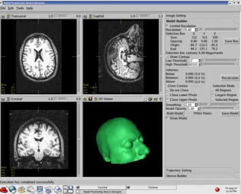
3.16). Probes can be created and oriented on the images to give clinicians a better idea of the procedure at hand.

Figure 3.15: Current graphical user interface.

Figure 3.16: Fixture created based on a head model.

3.2.1

Fixtures

The fixtures that will be used for testing are created using a 3d printer (see Figure 3.19). This device is composed of two bins: one holding the powder plaster and another which is empty an will eventually hold the printed 3D model. Powder is moved from one bin to another with a roller and glue is placed with a printing head on the receiving bin. This is illustrated in Figure 3.20

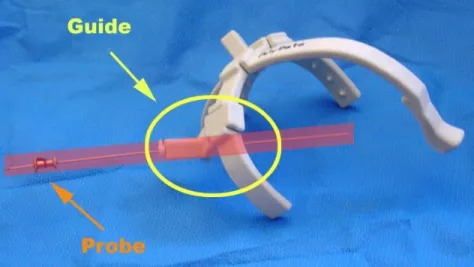
Figure 3.17: Fixture created using 3D printer with the guide to hold the probe.

Figure 3.19: Zprinter 310 three dimensional printer used to create the fixtures.

Figure 3.20: Zprinter 310 printing process.

3.3

Image domain segmentation techniques used in

med-ical MRIs.

3.3.1

Region growing

This algorithm starts with one or various seeds. From these a region grows by appending to each seed those neighboring pixels that have similar properties [9]. The main problem is to define the initial position of each seed. Usually in medical images such as MRI, the actual interest area is located near the center of the canvas; therefore the areas near the corners and sides can be considered the background and easily discriminated. This type of method is usually used to find tissue, for example the ventricles inside the brain can be segmented easily using image growing. There are problems when the region of interest is not completely enclosed which leads to undesired growth patterns.

3.3.2

Watershed

This technique starts with a topographical image in which region dissimilarities are encoded in higher altitudes [1]. Based on this map there are two algorithms that can be used for the segmentation. The first one floods the basins (minima) so the water level increases. When water from different valleys joins it is considered an edge. The other method is called rain-falling, and the regions are segmented according to the path a water drop follows to reach a minimum or basin. Both of these methods are displayed in Figure 3.21.

Figure 3.21: Watershed algorithms based on immersion (left) and rain-fall (right). The disadvantage of using watersheds is the over segmentation, therefore other meth-ods must be used in order to merge the regions. It is easier to identify regions by first using over-segmentation and then merging than having to detect the edges directly.

3.3.3

Active contours

Active contours ”snakes” were proposed by [10]. This algorithm starts with a curve that is placed on the image and transforms its shape adapting to the contours of the specified region (Figure 3.22). In order to use this algorithm a model of the contour must be created (image attractor). This can be done using user pre-segmented images or by using a low-level algorithm that would define areas in which the object is contained.

Figure 3.22: Example of how the snake adapts to the specific regions.

3.3.4

Active Shape Models

This technique was selected for the segmentation of the MR images and will be discussed in chapter 5.

3.4

Electronic and physical principles related to the

so-lution

The advanced mathematical tools used in electronic engineering are directly applied into image processing. In order to fully understand the ASM concepts such as the principal component analysis, eigen decomposition and the Mahalanobis distance must be defined.

Chapter 4

RESEARCH METHODOLOGY

4.1

Problem recognition and definition

The general problem was determined based on interviews with the head of the Radio surgery and radio Biology Laboratory Dr. Bova, and with assistant Scientist Dr. Rajon, main programmer for the rapid prototyping project.

The specific problem due to the MRI technical aspects was defined based on research papers and analysis of patient images.

4.2

Information gathering and analysis

Image segmentation techniques were reviewed from literature available at the lab-oratory and the university libraries. Current papers from different universities and institutes where also a large part of the research along with interviews with Dr. Rajon and other researchers from the department of electrical engineering.

4.3

Evaluation of the solution

approximately (CT numbers range from 0-4095). Because of these large differences a simple segmentation algorithm based on thresholding can be applied in order to determine the contour. The system implemented for the evaluation is shown in Figure 4.1.

Segmented image based on CT scan

Segmentented Image based on ASM

Segmented Image based on thresholding Mask

Comparison

Figure 4.1: Scheme for the evaluation of the segmentation algorithms

4.4

Implementation of the solution

In order to develop the solution several stages were completed. First of all a bib-liographical research on the most common segmentation methods in medical MRI was reviewed. Based on these papers and interviews at the department an adequate algorithm based on active shape models was designed.

4.5

Evaluation and re-design

At the end of this thesis several recommendations have been made for a more robust and accurate technique using the ASM.

Image processing techniques are constantly improving as well as the hardware used in their implementation.

Chapter 5

SOLUTION

5.1

Solution selection

A number of features can be used for image segmentation, these can be determined from image based information or from real world knowledge.

Segmentation is better understood in context with image recognition under the hu-man visual perception. Marr-Palmer’s computational vision framework in Figure 5.1 describes the process of object recognition. Image-based processing detects simple features like edges or corners. These salient features are then used by the surface-based processing block to create surfaces. Surfaces are assigned to objects in the object-based stage. The role and relationship with other objects in the scene is deter-mined in the last category-based processing block [1]. Feedback in the blocks reflect a bilateral and iterative process in human object recognition.

Retinal Image Image-based _Processing Surface-based _Processing Object-based _Processing Category-based _Processing

Figure 5.1: Marr-Palmer’s computational vision framework for human perception. Based on the first three stages of Marr-Palmer’s model, segmentation techniques may be grouped as follows:

• Image-based segmentation: uses only the information contained in the camera image to find regions defined by low-level homogeneity criteria.

• Object-based segmentation detects real-world objects, by grouping regions of the surface-based segmentation using high-level knowledge.

As stated above image segmentation does not only depend on information given at the pixel level but also depends on a-priori knowledge. For example when creating surfaces it is expected that the edges be continuous lines, therefore if the segmentation at lower levels suggest divided edges these can be assumed as continuous in the surface detection block.

Each one of these categories can be subdivided [1]. Other categorizations do exist as the one used by [18]:

• Thresholding

– Threshold detection methods. – Optimal thresholding.

– Multi-spectral thresholding.

– Thresholding in hierarchical data structures.

• Edge-based segmentation – Edge image thresholding. – Edge relaxation.

– Border tracing.

– Border detection as graph searching.

– Border detection as dynamic programming. – Hough transform.

Figure 5.2 shows a typical MRI scan. The first aspect that needs to be considered is the MRI scanner itself. The gray values in images depend directly from the scanner that is being used as can be seen in Figure 5.3.

Figure 5.2: Example of an MRI scan.

Figure 5.3: Examples of two MR images taken from different scanners.

Because the images can be generated from arbitrary machines it is important to have a pre-processing block that will filter out most of the variations. For this project histogram equalization and a median filter where applied. A median filter has the property of preserving the location of the edges, which is not true for others such as the Gaussian filters. After filtering is completed the magnitude of the gradient is calculated in order to decrease small variations along the gray values and increase the salient features in the image.

image of the object scanned. It is easier seen during the process of a CT scan shown in Figure 5.4. During the scan radiation originated from the source doesn’t travel in a straight line and therefore hits the object at a certain angle, depending on the composition of the objects these rays may be re-oriented and combined. This will create an image that represents an average of the original. Basically each pixel in the final image can represent more than one structure. This effect can be decreased by using a higher resolution. The partial volume effect is more complex and only a general idea has been presented here.

Radiation

MRI scanners in the process of creating an image use the inverse Fourier transform. This will cause repetitions of the original scan to appear. Figure 5.5 shows a scan at the top of the head in which the smaller oval represents the top portion and the larger shape around it is actually the bottom part of the head near the lips reappearing on the higher slices.

This last image shows another problem in MR imaging. There is a considerable signal loss as the scans near the top of the head in some cases the skin border may appear discontinuous because of this attenuation.

Because of all the variables and different scenarios present in a MRI scan, prior in-formation becomes an important factor to consider when designing the segmentation algorithm. Image based techniques only refer to pixel level information, therefore if the borders are not continuous or there is great attenuation these methods are prone to fail. Region-based methods such as split/merge, region growing and watersheds, are usefull as approximations to the border, but because no prior information is in-cluded the final result may contain odd head shapes, discontinuous edges or even false borders.

Figure 5.5: The inverse Fourier transform will cause bottom slices to reappear on the top slices.

Active contours are based on an energy minimization problem. A balance between the internal energy of the spline and the external energy obtained by the image is searched for. The internal energy refers to the elasticity and rigidity of the spline. The external energy involves the actual image information specially the salient features. The reason this method is likely to fail is that convergence on false edges is possible and there is no restriction on the shapes that may form when using these methods. For example, at slices near the eye level convergence on the brain cortex is highly probable.

Various combinations of the methods mentioned above are possible, for example watersheds or region growing techniques can be used to determine and approximate location of the head skin contour this approximation can be used to initialize an active contour in order to compensate for the discontinuous borders. But once again there are no constraints on the shapes generated.

defor-mations considered during the training stage. This method of segmentation includes real world knowledge by using examples of head contours.

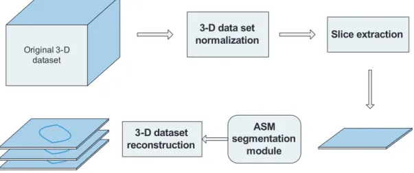
Image segmentation is only part of the project. Figure 5.6 shows a block diagram of the implemented solution divided into 4 modules:

• Pre-processing of the 3-D dataset.

• Offline creation of the shape and profile models.

• The active shape model module.

Original 3-D dataset

These slices don’t necessarily have the same

spacing between them

3-D data set re-interpolation

Re-interpolated to equal spacing User defined thickness

The orientation of the head is corrected based on the

AC, PC, MCL Re-oriented

& Re-interpolated

3-D dataset

Slice extraction segmentation ASM

module

3-D dataset reconstruction

5.2

Active shape models

A shape model can be expressed in general as:

X =f(b) (5.1)

Changing the values of b will generate new values for X which are determined by the model f, therefore b can be considered a descriptor of X. In the case of shape models the variation of the b parameters will generate new shapes and if the values ofb are constrained, only certain shapes may be expressed.

Shape is considered as the quality of a configuration of points which is invariant under some transformation. The similarity transformations (translation, rotation and scaling) are considered for 2-D and 3-D shapes.

Shapes can be expressed as a set of n paired coordinates (x, y):

x= (x1, y1),(x2, y2),(x3, y3)· · · (5.2) Rearranging the elements in equation 5.2 allows shapes to be expressed as a 2n

dimensional vector:

ASM capture the shape variations of an object into a model by using principal com-ponent analysis (PCA). This is a method for identifying patterns in data and once they have been found this data can be compressed. The method for PCA is detailed here.

5.2.1

Principal Component Analysis (PCA)

In order to use the principal component decomposition there are several steps. In this case shapes are expressed using the 2n dimensional vector format.

The second step consists in calculating the covariance matrix. The covariance be-tween 2 variables expresses how these variables vary in relation to each other. The covariance matrix can be calculated from the expression:

S= 1

wheres, is the number of shapes described using the 2n dimension vectors.

The third step is to calculate the eigenvectors and eigenvalues of the covariance ma-trix. The normalized eigenvectors represent the direction in which the data varies in relation to the mean. The eigenvalues refer to how much of the data varies in the direction of the corresponding eigenvector. Figure 5.7 shows a cloud of 3D data points.

Figure 5.7: Illustration of the eigenvectors for a set of 3D points. Because there are 3 dimensions the covariance matrix S is:

S=

to the variance in each dimension. Therefore√λ =S.D., where S.D. is the standard deviation for that dimension.

The number of eigenvectors will be the same as dimensions in the matrix. For the distribution 3D points in Figure 5.7 the eigenmatrix is:



For which the eigenvectors are organized as columns vectors:

e1 =

Each one of these vectors has an associated eigenvalueλ1_{, λ}2_{, λ}3_{. The original dataset} may be expressed as a combination of the mean value and a weighted sum of the eigenvectors:

X= ¯x+ ΦB (5.8)

In this case the column vector B represents the weights for the dimensions in the eigenvectors.

If we consider the data in Figure 5.7, the variation occurs mainly along two dimen-sions therefore one of the eigenvectors can be ignored, this eigenvector will corre-spond to that which has the lowest eigenvalue and thus expresses the least variance. This determines the fourth step which is to consider only the eigenvectors that rep-resent most of the variance in the dataset. This will allow for data compression by multiplying each value in the dataset by the truncated eigenmatrix.

PCA is fundamental in understanding the development of ASM. In this case the vectors will not be 2 or 3 dimensional, they will have twice as many dimensions as points used to describe the shapes.

5.2.2

Shape modelling

The main idea behind the ASM is being able to represent shape variation in a compact model.

First the mean shape is determined, along with the covariance matrix and its eigen decomposition. This allows shapes to be expressed using the model:

x≈x¯+ ΦB (5.10)

where, Φ = (e1| · · · |et)

The number of eigenvectors or modes considered in the model can be chosen based on the percent of variance expressed. In the implementation of the ASM the eigenvectors where arranged in descending order considering the respective eigenvalues. The number of modes used for the model where those that when added expressed 96% of the total variance.

The model is created by using a set of training shapes that will define the matrix Φ. If the number of training shapes used is less than the dimensions of the shape then the number of eigenvectors will be equal to the number of training shapes [3]. This model can also be used to generate new shapes by varying the parameters in the B column vector. The elements in this vector will weigh a dimension in each eigenvector as seen in equation 5.11:

x= ¯x+ ΦB

The first dimension of the shape x1 can be expressed as the mean plus a weighted sum of the first element in every eigenvector:

Therefore each shape can be characterized by its correspondingB vector. In order to determine a plausible shape the distribution of theb elements must be calculated. In this case it will be assumed that the elements in the B vector are independent and Gaussian. This means that all plausible shapes will be defined byBvectors for which all elements have been constrained to:

−3·S.D. < bi <+3·S.D.

−3·√λi < bi <+3

√

λi

(5.13)

The assumption that the elements in theB vectors are Gaussian is valid to represent the shapes of head contours because the variation is continuous. If the training set were instead shapes that showed only two distant possible variations then the probability density function for the b elements would show 2 spikes for which any of the values in between would generate invalid shapes.

By varying the elements of the B vector under the constraints, new shapes can be created. Figure 5.8 shows how the variation of each of the dimensions affects the mean shape, for a case in which the shapes are hands.

These shapes are defined by a group of points which are selected based on specific landmarks. The location of these landmarks is a complex problem specially if done automatically.

5.2.3

Landmarks

Landmarks are points that can be specifically located from one training image to another [3] (Figure 5.9), which means there is a correspondence between the points. The labeling of the training shapes can become a tedious task if done manually for 2D or 3D datasets. Some authors have used a minimum description length approach to select the landmarks automatically with promising results [16].

Main landmarks Intermediate landmarks

Figure 5.9: Landmark assignment near the tip of the nose.

For this project manual point correspondence was used. The simplicity of the human head contour allowed for an easy identification of important anatomical landmarks such as the tip of the nose and the eyes. Other methods used for automatic landmark placement in medical imaging combine the use of registered CT and MR images. Skin surfaces can be easily identified in CT scans, but they will not match the MRI scan entirely because during the CT scan the patient is wearing a head ring, while during an MR scan the patients head is pushed against the table. The different scenarios for the scans will produce inconsistencies in the contour of the rear part of the head.

5.2.4

Training set

The training images must be selected carefully because they will determine the plau-sible shapes allowed by the model.

as seen in Figure 5.10. Because each patient has his or her own unique characteristics the shapes have arbitrary scaling, translations and rotations that must be normalized through out the set.

Figure 5.10: Distribution of the patients by age at treatment in the radiosurgery database at the McKnight Brain Institute.

In order to align the training set the following method has been implemented [3]:

1. Translate each example so that its center of gravity is at the origin.

2. Choose one example as an initial estimate of the mean shape and scale so that

|x¯|= 1

3. Record the first estimate as x¯0 to define the default reference frame. 4. Align all the shapes with the current estimate of the mean shape. 5. Re-estimate the mean from the aligned shapes.

6. Apply constraints on the current estimate of the mean by aligning it with x¯0 and scaling so that |x¯|= 1

7. If not converge, return to 4.

In order to align two shapes, x1 to x2, first, x1 and x2 are translated to the origin where the average angle and distance between every set of corresponding points is calculated, then shape x1 is re-oriented and scaled using these values, finally x1 is translated so the center of gravity of x1 matches the original center of gravity of x2. Other methods for shape alignment can be used to minimize distances between both shapes [7].

It is important to recall that this model expresses only shape variation. The algorithm that morphs the shape is discussed in the following section.

5.2.5

Model morphing

For the shape model to become active another stage is required. This stage is known as model morphing. It uses image-based information obtained from the training images (not specifically the shapes) to determine the best movements of each point in the shape. Figure 5.11 shows the main idea. In order to determine the new suggested shape the Mahalanobis distance is used.

In order to calculate the Mahalanobis distance a model for the magnitude of the gradient for the gray level values along the normal profile that intersects each point in the shape is determined. The profile for each point is calculated based on the adjacent points as shown in Figure 5.12.

Suggested variation

Original position

First point

Second point

Last point

Figure 5.12: Gray level profile creation based on adjacent points.

Therefore a vector g of size k will be assigned to each point and it will contain the magnitude of the gradient that has been divided by the sum of the elements to normalize (5.14):

where the index i corresponds to a specific point in the shape, j represents the training image on which the shape is located and l iterates through the elements in the specified g vector. With this in mind a g vector will be created for each point of the shape on each one of the shapes in the training set.

With this set ofg vectors a profile model can be created for each one of the points in the shape. Similar to the shape model, a meangvector¯gi and covariance matrixSgi is

calculated for each point. These models are created based on a profile that contains

k values of gray levels. Once the mean g vectors and covariance matrix have been calculated the Mahalanobis distance of any other g vector of size k can be calculated by using (5.15):

f(gi) = (gi−g¯i)·Sg−1·(gi−g¯i)T (5.15)

To determine the displacement for a specific point a larger profile is selected of size

m. This larger profile is scanned using ak size profile that will be evaluated with the Mahalanobis distance. The vector that results in the smallest distance is considered to be the best fit and will determine the displacement for the point. This is illustrated in Figure 5.13.

constraints are applied. In order to apply these constraints the elements in the B

vector are determined from the current shape based on equation 5.16:

B= ΦT(x−x¯) (5.16)

k size profile vector

m size profile

vector m > k

Gray values

Scanned area

Figure 5.13: Profile scanning.

Because it was assumed that every element has an independent and Gaussian distri-bution, they have been limited to ±3S.D. therefore any element outside these limits will be forced to the maximum variation depending on their sign.

This is an iterative process between new shape suggestions given by the profile model and shape constraints determined by the shape model. At this point the algorithm is considered an active shape model. Figure 5.14 shows the suggested shape in red and the constrained shape in blue as it can be seen the ASM converges on the edges.

5.2.6

Initialization

An important factor that has great influence in the speed of convergence of the model is the initialization of the model. Similarity transformations will be applied to the shape x, therefore the shape converging on the image will be:

X =T(s,θ)·[x] +Tx (5.17)

The initial values for the scaling, rotation and translation define the shape initializa-tion.

Various methods may be used to determine the similarity transformation parameters, including region-based segmentation techniques and genetic algorithms, but in this case an easier approach was applied. Although initialization is an important decisive factor for the convergence of the ASM if a multi-resolution framework is used the importance of the initialization is decreased and the mean shape of all the training images can be used as a good starting point.

5.2.7

Multi-resolution framework

The multi-resolution framework consists in smoothing and subsampling the image at lower resolutions. This approach can be seen as a pyramid (Figure 5.15). First the shape is initialized at its mean value and placed on the lowest resolution, once the ASM has converged it is transferred to a higher resolution image this continues until the original resolution is reached. This method will increase the rate at which the ASM converges and will decrease the probability of an erroneous segmentation.

5.2.8

ASM features

Some of the advantages of using the ASM are [5]:

• The same algorithm is applicable to various problems by simply changing the training set.

• Expert knowledge can be captured and applied to the segmentation.

Figure 5.15: Multi-resolution framework.

The ASM have been able to detect objects in the presence of noise and warping of the shapes as seen in Figure 5.16.

Figure 5.16: Intermediate tests applied to the ASM during the implementation. The test image was transformed by adding noise, warping and smoothing.

5.3

3D dataset pre-processing

When a patient is placed in the MRI scanner (Figure 5.17), his body is moved through the magnetic field by sliding the table on which he is laying down. The slices ob-tained by the scan don’t necessarily have the same separation in the direction of the moving table (axial coordinate). The information given by the scanner contains an axial coordinate measured in millimeters which refers to the patients position on the table.

Figure 5.17: Setup in the MR scanning room.[8]

In order to create a uniformly spaced dataset the original set is linearly interpolated. The thickness of these slices may be adjusted by the user. The interpolation of the slices is required for the next step.

Another variant in MRI scanning is the position of the patients head. Figure 5.18 shows a sagittal cut in which the head is tilted. If these variations are large non linear transformations in the shape of the skin border will occur when the data set is sliced along the axial coordinate. These shapes cannot be expressed by the active shape model and therefore the segmentation will be flawed.

Figure 5.18: The patients head can be tilted as seen in the sagittal view (lower left).

5.3.1

Data set re-orientation

Before calculating the transformation matrix a coordinate system must be defined. The MRI scans provide information about the axial coordinate and the axial slice spacing in millimeters. The axial coordinate may have arbitrary values depending on the scanner and the position of the patient. The number of slices may also vary. The 3-D dataset will be interpreted in a world coordinate system. For which the line (0,0, z), will cross every slice at the center and the position of each slice along the z

axis will be given by its axial coordinate as seen in Figure 5.19, the dataset is spread in the direction of the x and y axis based on the spacing determined by the scanner. This spacing is constant for all axial slices.

X

Y Z (axial coordinate)

3-D dataset

Voxels

Figure 5.19: 3-D dataset interpreted in a world coordinate system.

Anatomical landmarks for image re-orientation

These landmarks correspond to the Anterior Commissure (AC), Posterior Commis-sure(PC) and mid sagittal line or mid center line(MCL). The typical location for these points can be seen in Figure 5.20.

The implementation of an automatic identification algorithm for these landmarks is also a complex problem. Figure 5.21 shows the landmarks selected manually, the problem becomes complex when even a specialist must undergo an iterative process to determine these points.

Figure 5.21: Identification of the landmarks.

The middle point between the AC and PC will be considered as the center of the head and the origin of the anatomical coordinate system. The transformation required to re-orient the data set will take place over this point.

The vector from PC to AC will determine the direction of the positive y axis, the z

axis is calculated based on the MCL and the vector determined by the cross product of y and z will define the x axis. Figure 5.22 shows the coordinate system based on the anatomical landmarks.

Equations (5.18) are used to determine the normalized vectors that describe the ori-entation of the head.

ˆ

x= yˆ×zˆ

kyˆ×zˆk

ˆ

y= AC−P C

kAC−P Ck

ˆ

z = (M CL−P C)−yˆ[(M CL−P C)·yˆ]

k(M CL−P C)−yˆ[(M CL−P C)·yˆ]k

Z

Figure 5.22: Coordinate system defined by the anatomical landmarks.

With these equations the relative angles between both coordinate systems are known and can be used to determine the transformation matrix. To do so three methods that can be applied:

• Direction Cosines.

• Euler angles.

• Euler Parameters.

The use of the direction cosines is considered to be a brute-force approach and is not applicable to video rendering or 3D graphics. Figure 5.23 shows coordinate systems F1 and F2, where F2 is the result of transforming F1 using the direction cosines matrix.

X1

In order to determine the direction cosines matrix the angle between the axis of both coordinate systems must be known, these can be calculated using the normalized vectors obtained from the AC, PC and MCL.

To reduce the number of computations when the dataset is transformed the inverse transformation is used. Each pixel position in the re-oriented system F2 will be transformed back to F1 and interpolated using trilinear interpolation 5.20.

InterpolatedV alue =B0·(1−x)·(1−y)·(1−z) surround the point that will be interpolated as can be seen in Figure 5.24.

X

Y Z

B0

B1 B2

B3 B4

B5 B6

B7

Figure 5.24: Basics of trilinear-Interpolation.

5.4

3D Dataset reconstruction

Chapter 6

RESULTS AND DISCUSSION

6.1

ASM overview

Figure 6.1 shows the initialization of the ASM. The average similarity transformations in the training set were used for the initialization. There were 113 points used to describe the contour of the head. The first tests were done with only 56 points. The results obtained were poor, the nose curvature wasn’t described correctly and therefore appeared as jagged lines in the final segmented image.

Figure 6.1: Active shape model initialization.

In order to obtain better results the head was divided into 2 regions based on the AC-PC plane. One model was created for the top of the head and another for the bottom which includes mostly the nose and the lips of the patient depending on the amount of information available from the scan.

• Above the AC-PC plane.

– Original 512 x 512 resolution – 256 x 256 resolution

– 128 x 128 resolution

• Under the AC-PC plane.

– Original 512 x 512 resolution – 256 x 256 resolution

– 128 x 128 resolution

Each one of these models includes both the shape model and the profile model. One of the main advantages of ASM is the fact that the number of training images can be nearly unlimited because the creation of the model is done offline. The end result is simply the mean shape, the eigen decomposition, a mean profile vector and an inverted covariance matrix list for the profile model.

Figures 6.2, 6.3 and 6.4 show the process of convergence of the ASM at different res-olutions. The iterations start with an image that has been downsampled and filtered using a Gaussian mask to a resolution of 128x128 pixels. In this case convergence occurred in 10 iterations. Convergence can be defined when the distance between the expected shape and the original shape reaches a threshold.

Once the ASM has converged the resolution is increased until the original resolution is achieved.

One of the advantages of using these 3-D datasets is that the variation between two consecutive slices is minimum. This was exploited during the implementation by using the multi-resolution framework only on the slice defined by the AC-PC plane. The next slices used the previous position and only the 512x512 model was applied.

Figure 6.3: Active shape model converging at a resolution of 256x256.

Figure 6.4: Active shape model converging at a resolution of 512x512.

6.2

Results at specific depths in the brain

The following sections show the final position of the ASM at different depths in the head.

6.2.1

Over the AC-PC plane: Top of the head

One of the major problems of using thresholding is the effect of signal loss in slices near the top of the head. Figure 6.5 shows convergence of the ASM even though the borders are faded and discontinuous. This can also be appreciated in the 3-D models shown in Figure 6.11.

Figure 6.5: ASM converging on a slice near the top of the head.

6.2.2

Under the AC-PC plane: nose curvature

After the top part of the head has been segmented the model is switched (nose model). The main characteristic of these slices is the shape of the nose. Figure 6.6 shows the convergence of the ASM on one of these slices. In this case the nose has been well detected, but because of the anatomy of the nose false border detection becomes an eminent problem as will be shown in the next section.

Figure 6.6: ASM converging on a slice under the AC-PC plane.

6.3

Comparison obtained using thresholding and ASM

using thresholding methods and ASM will be considered in the following.

In order to compare both methods, registered CT and MRI scans were used. But the entire contour was not accounted for, only the patients face was used to compare the results because the rear of the head usually does not match between the CT and MRI. This occurs because during the MR scan the patient is laying down on his back with his head against the table, while during the CT scan the patients head is surrounded by the stereotactic headring.

The figures shown in this section correspond to the mask obtained from both seg-mentation techniques over-imposed on the mask generated by the CT, which is used as the reference point for comparisons.

6.3.1

Over the AC-PC plane: Top of the head

As a final result of the segmentation process the program is able to deliver either a binary mask of the skin contour or a boundary conserving the rest of the original data. For the comparisons a binary mask was created for both the thresholding and ASM.

Figure 6.7 shows the superposition of the ASM and thresholding results over to copies of the CT reference. Both segmentation techniques seem to return similar results. The problem with thresholding is more clearly viewed in the 3-D images in the following section.