Comparison of Magneto Rheological Damper Models Edición Única

Texto completo

(1)

(2) INSTiTUTO T E C N O L O G I C O Y DE ESTUDiOS SUPERJORES DE M O N T E R R E Y MONTERREY. CAMPUS. G R A D U A T E P R O G R A M IN M E C H A T R O N I C S A N D INFORMATION. TECHNOLOGIES. TECNOLOGICO DE MONTERREY. COMPARISON. OF MAGNETO-RHEOLOGICAL DAMPER. MODELS. THESIS P R E S E N T E D IN PARTIAL F U L F I L L M E N T O F T H E REQUIREMENTS. FOR T H E D E G R E E O F :. M A S T E R O F S C I E N C E IN A U T O M A T I O N BY:. JAVIER A N T O N I O R U I Z C A B R E R A. MONTERREY. NUEVO. L E O N , M E X I C O D E C E M B E R 2010.

(3) INSTITUTO TECNOLÓGICO Y DE ESTUDIOS SUPERIORES DE MONTERREY MONTERREY CAMPUS GRADUATE PROGRAM IN MECHATRONIC S AND INFORMATION TECHNOLOGIES. COMPARISON OF MAGNETO-RHEOLOGICAL DAMPER MODELS. THESIS PRESENTED IN PARTIAL FULFILLMENT OF THE REQUIREMENTS FOR THE DEGREE OF:. MASTER OF SCIENCE IN AUTOMATION BY. JAVIER ANTONIO RUIZ CABRERA. MONTERREY, N U E V O LEON, MEXICO, D E C E M B E R 2010.

(4) ©Copyright by Javier Antonio Ruiz Cabrera, 2010 All Rights reserved.

(5) INSTITUTO TECNOLÓGICO Y DE ESTUDIOS SUPERIORES DE MONTERREY DIVISIÓN OF MECHATRONICS AND INFORMATION TECHNOLOGIES GRADUATE PROGRAM IN MECHATRONICS AND INFORMATION TECHNOLOGIES. The members of the thesis committee hereby approve the thesis of Ing. Javier Antonio Ruiz Cabrera in partial fulfillment of the requirements for the degree of. M A S T E R OF SCIENCE IN AUTOMATION. Thesis Committee:. Gerardo A. Castanon A., Ph. D. Director of Automation and Electronics Graduate Programs, DMTI December 2010. iii.

(6) Comparison o f Magneto-Rheological D a m p e r. Models. BY Javier Antonio Ruiz. Cabrera. THESIS. Presented to the Graduate Program in Mechatronics and Information Technologies This Thesis is a partial requirement for the degree of MASTER OF SCIENCE IN AUTOMATION. INSTITUTO TECNOLÓGICO Y DE ESTUDIOS SUPERIORES DE MONTERREY. MONTERREY, NUEVO LEÓN, MEXICO, DECEMBER 2010. iv.

(7) Dedication. A Dios: A quien debo todos mis logros.. A mis papas: Quienes siempre me ensenaron el camino correcto. Gracias por su amor y apoyo incondicional. Mis logros son un reflejo de su trabajo.. A Valerie: M i amada companera. Gracias por ser parte de mis suefios. Tu amor me da fuerzas para conseguir nuestras metas.. A toda mi familia: Porque puedo contar con ustedes. Siempre los llevo en el corazon.. v.

(8) Acknowledgements I would like to thank Dr. Ruben Morales, whose encouragement and valuable guidance enabled me to complete my research work. In addition, I would like to offer my regards to Jorge Lozoya for providing the experimental data for this work and to Dr. Luis Garza and Dr. Ricardo Ramirez for their time and contributions to the present report. Lastly, I thank all of those who supported me in any respect during the completion of my degree and final research. Thanks to my fellow classmates for their invaluable friendship and the unforgettable times we shared.. - Javier Antonio Ruiz Cabrera. vi.

(9) Abstract. The design of automotive suspension systems is concerned with ride comfort and handling performance of the vehicle. In the last decade, semi-active suspension systems have been greatly analyzed for automotive applications as they offer the reliability of passive devices, but maintain the versatility and adaptability of active systems. Semiactive Magneto-Rheological {MR) dampers present a viable choice for suspension systems. In an MR damper, the damping characteristics can be modified with the application of a magnetic field to the coil inside the tube of the device. Although MR dampers are greatly promising for the control of vehicle suspension systems, their major drawback lies on their non-linear and hysteretic behavior. This behavior makes it a challenge to develop a model for the system. Furthermore, the first step in designing a control strategy for a suspension system is modeling the behavior of the damper in an accurate manner. The present research is focused on the modeling of an MR damper. The problem statement is centered on what type of model of an MR damper can be developed, which can accurately predict the highly non-linear behavior of the system and can be optimal for online control. For this purpose, various sets of experimental data were obtained from an industrial MR damper. Then, four state-of-the-art MR damper models were trained, analyzed and compared using quantitative and qualitative techniques. Each of the models was selected from four main modeling approaches, phenomenological, semi-phenomenological, black-box, and fuzzy-based. By the end of the research, a novel model for an MR damper was presented, which combined fuzzy techniques with semi-phenomenological modeling. The results showed that the proposed structure was able to accurately predict the behavior of the MR damper and was suitable for control purposes. The final results can be greatly applicable to the automotive industry, where better comfort and handling control systems could be developed. In addition, the results could be useful to the vast number of industries and applications where MR dampers are employed.. vii.

(10) Contents 1. 1.1. 2. 1. Introduction Presentation. '. 1.2. Problem Statement. 3. 1.3. Objectives. 3. 1.3.1. General Objective. 3. 1.3.2. Specific Objectives. 3. 1.4. Justification. 4. 1.5. Hypothesis. ^. 1.6. Research Strategy. 4. 1.7. Thesis Outline. 5. Literature Review 2.1 State-of-the-Art Models 2.1.1 Phenomenological (P) Models 2.1.2 Semi-Phenomenological (S-P) Models. ^ 6. 6. 7. 2.1.3. Black-Box Models. 1 0. 2.1.4. Fuzzy-Based Models. *. 2.1.5. Comparison. 2. ^. 2.2. Previous Work. 1 6. 2.3. Opportunities. 1 7. 2.4. Summary. 1 8. 19. 3. Experiments 3.1 Design of Experiments 3.1.1 Electric Current Patterns 3.1.2 Displacement Pattern 3.2 Experimental Setup 3.3 Signal Conditioning 3.3.1 Noise Filter 3.3.2 Discrete Derivative 3.4 Experimental Results 3.5 Summary. 1 9. 1 9. 2 1. viii. 2. 2. 2. 2. 2. 2. 2. 3. 2. 3.

(11) 4. Results. 25. 4.1. Error Calculation. 25. 4.2. ARX Model. 26. 4.3. Semi-Phenomenological {S-P) Model. 29. 4.4. Phenomenological (P) Model. 31. 4.5. Fuzzy-Based Model. 33. 4.6. Non-Linear Fuzzy-Based Model. 35. 4.7. Summary. 36. 5 Analysis and Comparison of Results 5.1. 6. 38. Best Models. 38. 5.1.1. A R X Model. 39. 5.1.2. S-P Model. 41. 5.1.3. P Model. 41. 5.1.4. Fuzzy-Based Model. 43. 5.1.5. Non-Linear Fuzzy-Based Model. 43. 5.2. Discussion. 45. 5.3. Summary. 47. Conclusions. 49. 6.1. Final Conclusions. 49. 6.2. Future Work. 50. A Experiments A . l Experimental Setup. ^4 54. A. 1.1. Experimental System. 54. A. 1.2 A. 1.3. Actuation System Control System. 54 54. A. 1.4 Data Acquisition System A.2 Experimental Data Sets. 55 55. A. 3 Discrete Derivative. 56 5 9. B Identified Coefficients B. l. 5 9. ARX Model. B.2 S-P Model. 6 1. B.3 P Model. 6 1. C Fuzzy-Based Model. 6 4. D Non-Linear Fuzzy-Based Model. 74. E Published Works. 7. ix. 7.

(12) List of Tables 1. Description of variables. xiii. 2. Description of variables continued. xiv. 2.1. Comparison of Models. 16. 3.1 3.2. Roughness coefficients for power spectral density functions of road profiles Experimental data sets. 21 24. 4.1. Identification RSSE and ESR for the passive ARX model. 26. 4.2. Identification RSSE and ESR for the semi-active ARX model. 28. 4.3. Identification RSSE and ESR for the passive S-P model. 29. 4.4. Identification RSSE and ESR for the semi-active S-P model. 30. 4.5. Identification RSSE and ESR for the passive P model. 31. 4.6. Identification RSSE and ESR for the semi-active P model. 32. 4.7. Identification RSSE and ESR for the fuzzy-based model. 34. 5.1. Average RSSE (lbf) by model and experimental data set. 38. 5.2. Average ESR by model and experimental data set. 39. B. 1 Identified coefficients for the passive ARX model B.2 Identified coefficients for the semi-active ARX model. 60 60. B.3 Identified coefficients for the semi-active ARX model continued. 60. B.4 Identified coefficients for the passive S-P model B.5 Identified coefficients for the semi-active S-P model. 61 61. B.6 Identified coefficients for the semi-active S-P model continued. 62. B.7 Identified coefficients for the passive P model. 62. B.8 Identified coefficients for the semi-active P model B.9 Identified coefficients for the semi-active P model continued. 62 63. D. 1 Identified coefficients for the non-linear fuzzy-based model. 74. x.

(13) Table 1. Description of variables. The variables are shown in order of appearance. Variable. Description. Model. Units. x(t). Linear displacement of the MR damper. x(t). Linear velocity of the MR damper. In/s. Linear acceleration of the MR damper. In/s. m i(t) V(t) F(t). In. Electric current on the coil of the MR damper. A. MR damper voltage. V. MR damper output force. lbf. Estimated MR damper force. lbf. F(t). Second derivative of F(t). lbf/s. F(t). First derivative of F(t). F(t),. F. est. 2. 2. Ibf/s. F*(t). Fifth power of F(t). lbf. F*(t) K. Third power of F(t). lbf. 5. 3. Pi Sj. Parameters for the model. Eq. 2.1. Parameters for the model. Eq. 2.2. -. CO Cl k. Coefficient for the viscous damping at large velocities. Eq. 2.2. lbfs/in. Damping coefficient for the roll-off at low velocities. Eq. 2.2. lbfs/in. 0. Stiffness control coefficient for large velocities. Eq. 2.2. N/cm. ki. Accumulator stiffness coefficient. Eq. 2.2. N/cm. T. Discrete sample Total number of discrete samples. Initial displacement of spring ki. Eq. 2.2. N/cm. Evolutionary coefficients for the model. Eq. 2.2. A!. Dynamic yield force coefficient. Eq. 2.3. A. 2. Post-yield viscous damping coefficient. Eq. 2.3. ^3. Pre-yield viscous damping coefficient. Eq. 2.3. V. Hysteretic critical velocity coefficient. Eq. 2.3. X Cyj. Hysteretic critical displacement coefficient. Eq. 2.3. -. Viscous coefficient for the model. Eq. 2.4. lbf - s/in. kyj. Stiffness coefficient for the model. Eq. 2.4. lbf/in. Hysteretic variable. Eq. 2.4. x. 0. z(t),y(t). 0. 0. Zw(t) a fo 0 8 Ljn. Positive acceleration parameters for the model. Eq. 2.5. Negative acceleration parameters for the model. Eq. 2.5. -. Scale factor of hysteresis. Eq. 2.4. Damper force offset coefficient. Eq. 2.4. Hysteretic slope coefficient. Eq. 2.4. Hysteretic width coefficient. Eq. 2.4. Stiffness coefficient. Eq. 2.5. lbf/in. Positive acceleration MR damper force. Eq. 2.5. lbf. Negative acceleration MR damper force. Eq. 2.5. lbf. Coefficient for the pre-load of the accumulator. Eq. 2.6. -. Coefficient for the viscous damping. Eq. 2.6. lbf-s/in. k. L. F {t) P. fe Cb. xiii.

(14) Table 2. Description of variables continued Variable fy h XQ m. Description. Model. Units. Yielding force coefficient. Eq. 2.6. lbf. Shape coefficient for the model. Eq. 2.6. -. Hysteretic velocity coefficient. Eq. 2.6. in/s. Virtual mass coefficient for the model. Eq. 2.6. lb. Coefficients for the model. Eq. 2.7. bij, b2j Fk-j. Discrete value of the force of the MR damper at sample k — j. %k-j. Discrete value of the displacement of the MR damper at sample k — j. Xk—j. lbf in. Discrete value of the velocity of the MR damper at sample k — j. in/s. CLj. Coefficients for the model. Eq. 2.8. -. LlNj Lij. Input layer neurons of the neural network. Fig. 2.4. -. First hidden layer neurons of the neural network. Fig. 2.4. -. Second hidden layer neurons of the neural network. Fig. 2.4. -. Output layer neurons of the neural network. Fig. 2.4. -. Aj. Fuzzy sets for the first input of the fuzzy-based model. Fig. 2.6. -. Bj. Fuzzy sets for the second input of the fuzzy-based model. Fig. 2.6. -. Fuzzy sets for the third input of the fuzzy-based model. Fig. 2.6. -. Output functions of the fuzzy model. Fig. 2.6. -. Degree of fitness of the fuzzy rules. Fig. 2.6. -. Normalized degree of fitness of the fuzzy rules. Fig. 2.6. -. Output parameters of the model. Fig. 2.6. -. Uniformly distributed white noise. Eq. 3.1. -. Number of constant amplitude samples. Eq. 3.1. -. Normally distributed random number. Eq. 3.2. Hz. Loj M M M fj(x,x, i, t) Ci. W Wrij t. Oj,qj,n,Uj e(t). NICPS. Probability variable. Eq. 3.2. S(f) Cr. Power spectral density of the elevation of the road profile. Eq. 3.3. Roughness coefficient of the road profile. Eq. 3.3. Ncr. Constant coefficient corresponding to the roughness of the road profile. Eq. 3.3. Speed of the vehicle. Eq. 3.3. in/s. a. Vc. 2. ft /cycles/ft. Number of cycles per feet. Eq. 3.3. cycles/ft. Random phase angle normally distributed between 0 - 27r. Eq. 3.4. -. i Au. Frequency within the interval of S(f). Eq. 3.4. -. Frequency increment. Eq. 3.4. -. Minimum frequency for the spectrum. Eq. 3.4. -. Wmax N. Maximum frequency for the spectrum. Eq. 3.4. -. max. Eq. 3.4. -. Transfer function for the low-pass filter. Eq. 3.5. -. Ux <t>j u. f. GLPF(S). Total number of frequency intervals within w j „ — u> m. M. Fuzzy sets for the non-linear fuzzy-based model. Fig. 4.13. -. W. Degree of fitness of the fuzzy rules. Fig. 4.13. -. Output functions of the non-linear fuzzy model. Fig. 4.13. -. Fj. Fj. fj{x, x, i). xiv.

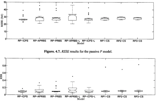
(15) List of Figures 1.1. MR damper configuration. 2. 1.2. Force- velocity behavior of an industrial MR damper.. 2. 2.1. Diagram of the semi-phenomenological model presented in [1]. 7. 2.2. Diagram of the semi-phenomenological model presented in [2]. 8. 2.3. Diagram of the semi-phenomenological model presented in [3]. 2.4. Three layer ANN with three inputs and one output. 11. 9. 2.5 2.6. Fuzzy system block diagram Structure of a first-order TSK fuzzy-based model. 12 14. 3.1. Block diagram of the experimental setup. 23. 3.2. Description of experiment RP-ICPS. 24. 3.3. Description of experiment RP3-CS. 24. 4.1 4.2. RSSE results for the passive ARX model ESR results for the passive ARX model. 27 27. 4.3. RSSE results for the semi-active ARX model. 28. 4.4. ESR results for the semi-active ARX model. 28. 4.5. RSSE results for the semi-active S-P model. 30. 4.6 4.7. ESR results for the semi-active S-P model RSSE results for the passive P model. 30 32. 4.8. ESR results for the passive P model. 32. 4.9 RSSE results for the semi-active P model 4.10 ESR results for the semi-active P model. 33 33. 4.11 RSSE results for the fuzzy-based model. 34. 4.12 ESR results for the fuzzy-based model. 34. 4.13 Non-linear fuzzy-based model 4.14 RSSE results for the non-linear fuzzy model. 35 36. 4.15 ESR results for the non-linear fuzzy model. 36. 5.1. Experimental and estimated damper force by the selected ARX model. 39. 5.2 5.3. Experimental and estimated F-v behavior of the selected ARX model Experimental and estimated damper force by the selected S-P model. 40 41. 5.4 5.5. Experimental and estimated F-v behavior of the selected S-P model Experimental and estimated damper force by the selected P model. 42 43. 5.6. Experimental and estimated F-v behavior of the selected P model. 44. xi.

(16) 5.7. Experimental and estimated damper force by the selected fuzzy-based model. 45. 5.8. Experimental and estimated F-v behavior of the selected fuzzy-based model. 46. 5.9. Experimental and estimated damper force by the selected non-linear fuzzy-based model. 47. 5.10 Experimental and estimated F-v behavior of the selected non-linear fuzzy-based model. 48. A.l. 56. Description of experiment RP-APRBS. A.2 Description of experiment RP-PRBS. 56. A.3 Description of experiment RP-APRBS-L. 57. A.4 Description of experiment RP-ICPS. 57. A.5 Description of experiment RP1-CS. 57. A.6 Description of experiment RP2-CS. 58. A. 7 Velocity calculation using Simulink. 58. B. l. Identification of the coefficients for the models. 59. C. l. Fuzzy-based model validation. 64. D. 1 Non-linear fuzzy-based model validation. 76. xii.

(17) Chapter 1. Introduction 1.1. Presentation. With the development of science and technology for automobiles and the continuously increasing need for safety and comfort, great attention has been drawn to automotive suspension systems. The primary concerns that a suspension system has to address are ride comfort and handling performance of the vehicle. Ride is primarily associated with the ability of a suspension system to accommodate vertical inputs. On the other hand, handling relates more to horizontal forces acting through the center of gravity and moments acting through the wheels. Among automotive suspensions, three main groups can be identified. The first, passive suspension systems, are the most widely used systems in vehicles. As their name suggests, the role of a passive suspension system is to withstand perturbations without the use of an external power supply or feedback control system. Thus, passive suspensions are designed as a compromise between ride comfort and handling performance. The second group is active suspension systems. Active systems are meant to provide independent treatment of perturbations using inertial forces through active control of some of the suspension system functions. In theory this means that the mentioned compromise in passive suspension systems can be eliminated. Active suspension systems, however, usually involve a continuous power supply, fast-acting mechanical devices, complex control algorithms, and closedloop control systems. The final group is that of semi-active suspension systems. These systems offer the reliability of passive devices, but maintain the versatility and adaptability of active systems. A semi-active suspension can be adjusted in real time, but cannot input energy into the system being controlled. Hence, the force delivered by the suspension is constrained to be proportional and opposite to the elongation speed of the damper. Nonetheless, the power requirement of these systems is considerably lower than that of an active system. In semi-active suspension systems for vehicles, the most commonly used damping devices are mono-tube dampers. A widely investigated mono-tube semi-active damper is the one denominated Magneto-Rheological (MR) damper. An MR damper is a non-linear dynamical system where the inputs can be the elongation speed and an electric current. The electric current is the control input that modulates the damping characteristic of the MR fluid through the variation of a magnetic field. The output is the force delivered by the damper. Fig. 1.1 illustrates the main components of an MR damper. MR fluids are non-colloidal suspensions of particles with a size on the order of a few microns [4]. These fluids are unique due to their ability to change their properties reversibly between fluid and solid-like states upon the. 1.

(18) 2. Figure. 1.1. MR damper configuration. The coil is connected to an external power supply. The MR fluid is energized as it passes through the annular gaps. application of a magnetic field. As discussed in [5], when a certain magnetic field is applied to an MR fluid, the particles in the fluid become polarized and form polarization chains in the direction parallel to the applied field. The mechanical energy needed to yield these chain-like structures increases proportional to the applied magnetic field, resulting in a field dependent yield stress. This region is referred to as the pre-yield region. When the external shear stress is increased and exceeds a certain value, the polarization chains will be broken and MR fluids start to flow like regular Newtonian fluids. This last region is referred to as the post-yield region. If the shear stress is gradually decreased again, the broken polarization chains will tend to reform, but with a stress value less than the one with which they were broken. Thus, a hysteretic behavior is observed on the material. Fig. 1.2 shows the force-velocity behavior of an industrial MR damper under various constant electric current inputs.. (a). (b). Figure. 1.2. Force-velocity behavior of an industrial MR damper. On the left side, the force is plotted against the velocity and electric current. On the right side, the force is plotted against the velocity for various constant electric current inputs. As mentioned in [1], in the past decade there has been an increasing interest of scientists and engineers on MR fluid dampers and their applications. MR dampers have been utilized in a broad range of areas. Large MR.

(19) Presentation. 3. damping systems have been studied for civil engineering applications when damping is required to withstand the high vibrations generated by earthquakes [6]. Also, vibration control systems that include MR dampers have been developed for railcar comfort [7]. On the biotechnological side, MR dampers are being studied as part of intelligent prosthesis [8] and bionic legs [9]. According to [10], concerning the automotive industry MR fluids are appealing for vehicle suspension systems since they can operate at temperatures ranging from 40 to 150 °C with only slight variations in the yield stress. Additionally, MR fluids are almost insensitive to impurities and can be controlled with low voltages (12-24 V) and a current driven power supply outputting 1-2 A .. 1.2. Problem Statement. Although MR dampers are greatly promising for the control of vehicle suspension systems, their major drawback lies on their non-linear and hysteretic behavior. Furthermore, the first step in designing a control strategy for a suspension system is modeling the behavior of the damper in an accurate manner. High-accuracy black-box and semi-phenomenological models have been developed recently. The models utilize displacement, velocity, electric current, and, many times, old values of the damping force as process variables in order to predict the output force of the MR damper. Nonetheless, to accurately predict the output force of the MR damper, the models are required to include a high number of parameters or complex mathematical functions. Thus, the computational necessities of those models become non-practical for commercial online application. Due to the aforementioned, what type of model of an MR damper can be developed, which can accurately predict the highly non-linear and hysteretic behavior of the system and be suitable for online implementation of a control system? To answer this question, a broad spectrum of modeling techniques will be analyzed and employed. To obtain experimental data sets, a series of experiments will be carried out on a commercial MR damper . The experiments will be designed to test the behavior of the damper under various input profiles. Then, various MR damper models will be tested and validated using the experimental data. At the end of the research, an MR damper model will be proposed. 1. 1.3 1.3.1. Objectives General Objective. The general objective of the present research is to explore various models and modeling techniques for an MR damper in order to compare them and analyze their strengths and weaknesses based on experimental data.. 1.3.2. Specific Objectives. 1. Perform experiments on an industrial MR damper in order to obtain real data and useful information for model identification. 2. Test models that describe in a precise and simple manner the behavior of an MR damper. 3. Compare how the models predict the behavior of an MR damper, using established criteria. 4. Identify input patterns that allow a better identification of models for the MR damper. 5. Present novel techniques to model an MR damper. 'Thanks to Metalsa www.metalsa.cotn.mx.

(20) 4. 1.4. Justification. As mentioned before, the areas where MR dampers can be utilized abound. Over the past decade, sustained interest in MR devices has increased due to the controllable interface provided by the MR fluid inside the damper. This fluid enables the mechanical system to interact with an electronic controller, which can be used to continuously adjust the mechanical properties of the damper. Some examples of devices in which MR fluids have been employed include dampers, clutches, brakes, and transmissions [11]. Nonetheless, the development of an effective control algorithm is reliant on the accurate modeling of the system to be controlled. The MR damper system includes both the process and the actuator. Thus, the adequate characterization of this system has shown to be a challenge due to its highly nonlinear dynamic response [12]. The present research is motivated by the aforementioned challenge that involves the correct modeling of an MR damping system. Various models and modeling techniques will be analyzed in order to compare their strengths and weaknesses. In addition, the training input patterns utilized for the identification of models will be discussed. Moreover, a new model for an MR damper will be proposed. The obtained results could be applicable to the automotive industry, where better comfort and handling control systems could be developed. Also, the results could be useful to the vast number of industries and applications where MR dampers are employed.. 1.5. Hypothesis. The present research seeks to propose and compare models and modeling techniques for an MR damper. In consequence and based on the elements discussed in the previous sections, the following thesis statements are proposed. 1. Models for an MR damper can be developed, which can precisely describe its behavior. 2. There are certain modeling techniques that outperform the rest and help to develop precise and optimal models of an MR damper. 3. There are certain experimental input patterns that facilitate the identification of models for an MR damper.. 1.6. Research Strategy. The present research will be divided into four main areas. 1. First, the previous work done on modeling of MR dampers will be revised. Then, the literature review will be centered on the various modeling approaches and techniques that have already been used for modeling MR dampers. The review will be the starting point for selecting various models for comparison. 2. Second, experiments to be performed on a commercially available MR damper will be designed. Once the experiments have been defined, experimental data will be obtained using an industrial MR damper. 3. Third, various models for the MR damper will be trained using the generated experimental data. The models will be compared against each other by using various performance indexes and qualitative indicators. After comparing the models, a set of different modeling techniques will be analyzed and new models for the MR damper may be developed. 4. Fourth, based on the results, a novel modeling technique for the MR damper will be documented..

(21) Presentation. 1.7. 5. Thesis Outline. The present work is divided into six chapters and five appendixes. This chapter presented the introduction, problem definition, and general outline of the research. In Chapter 2, a literature review on the modeling of MR dampers is discussed. In Chapter 3, the design of experiments and experimental setup are described. In Chapter 4, the results obtained on the comparison of MR damper models are presented. In Chapter 5, the obtained results are analyzed and discussed. Finally, in Chapter 6 the final conclusions of the research are presented..

(22) Chapter 2. Literature Review A literature review on the modeling of MR dampers is presented. In the first section, the state-of-the-art models of MR dampers are discussed according to various modeling approaches. Next, a summary of previous work done on comparing MR damper models and training patterns is presented.. 2.1. State-of-the-Art Models. The models were divided into four different approaches: Phenomenological, Semi-Phenomenological, Black-Box, and Fuzzy-Based.. 2.1.1. Phenomenological (P) Models. Phenomenological models are obtained by analyzing the physical characteristics of the systems they seek to model. Thus, in this type of models the parameters can be said to have a physical interpretation. The model presented in [5] represents a phenomenological model based on the phase shifting dynamics of MR fluids. The authors based the analysis on the differential equations that characterize the behavior of the MR fluid as it flowed through the gap between the piston and the cylinder in the MR damper. The proposed model is shown in equation 2.1.. where the five parameters pj need to be determined under a given loading velocity x(t); F(t) is the generated force; 3. F(t) and F(t) are the first and second derivatives of the force, respectively; and F(t). 5. and F(t). are the third. and fifth powers of the force, respectively. Notice that the model is a second order differential equation, with five parameters, that uses the velocity and force as inputs. Using the experimental data employed in [1] (specified in the next section), the parameters for the model were identified using nonlinear least-squares approximation. After numerical experimentation, the authors concluded that the model that was constructed captured the hysteretic behavior of the damper precisely. In addition, hysteresis loops with various loading frequencies, applied field intensities, and excitation amplitudes were all modeled successfully by the proposed model. The authors commented that in the model, all the coefficients are to be assumed to be. 6.

(23) Literature Review. 1. dependent on the applied electrical current. That is, the coefficients should be functions of the applied magnetic field. This dependency is to be approximated by a polynomial of order 2 and must be identified from experimental data.. 2.1.2. Semi-Phenomenological (S-P) Models. Semi-phenomenological models combine the analysis of the physical characteristics of the systems and various mathematical techniques in order to model those systems. The model presented in [1] has been widely used to compare models for MR dampers. The authors modified a previously proposed structure in order to include the regions where the acceleration and velocity have opposite signs. The structure of the model is shown in Fig. 2.1 and in equation 2.2.. Figure. 2.1. Diagram of the semi-phenomenological model presented in [1].. where Co and ko represent the viscous damping and stiffness characteristics at large velocities, respectively, ci is the damping coefficient for the roll-off induced at low velocities. k\ and xo represent the accumulator stiffness and its initial displacement, respectively. Sj represents coefficients that are to be determined from experimental data. In addition, z(t) and y(t) are evolutionary coefficients for the model. The model can be seen to include 10 parameters, and be dependent on the displacement and the velocity. To validate the proposed structure, the authors calculated the prediction error as a function of time, displacement, and velocity. The experimental data explored sinusoidal, step, triangle, and pseudo-random displacement patterns with frequencies lower than 3 Hz. The electric current pattern was constant stepped increments. The model was capable of exhibiting a wide variety of hysteretic behaviors. Moreover, the model could be effectively employed for control algorithm development and for system evaluation. Nonetheless, the model does not include the effect of the varying electric current..

(24) 8. Continuing in the search of semi-phenomenological models, the one presented in [2] has been greatly analyzed in the past years. The proposed model is said to describe the bi-viscous and hysteretic behaviors of the MR damper with high precision. The structure is described in Fig. 2.2 and in equation 2.3,. Figure. 2.2. Diagram of the semi-phenomenological model presented in [2].. where A\ represents the dynamic yield force of the MR fluid. A2 and A3 are parameters related to post-yield and pre-yield viscous damping coefficients respectively. VQ and XQ denote the absolute value of hysteretic critical velocity and hysteretic critical displacement, respectively. In the equation, the model can be seen to use the displacement and velocity as inputs and only depend on five parameters. The experiments performed on the MR damper consisted on sinusoidal sweeps for the displacement and constant steps for the electric current. The authors used a non-linear least-squares algorithm in order to identify the coefficients of the model. The results obtained in the experimentation were said to prove the correctness of the proposed structure. In addition, the concise form of the model was mentioned as its best feature. Nevertheless, the authors did not use experiments in which the current varied over time to prove the effectiveness of the model under varying current scenarios. Although, the authors noted that parameter A3 could be said to be independent from the applied electrical current. Another semi-phenomenological model that is to be considered is the one presented in [3]. The model is intended to include the hysteretic force-velocity characteristic of the MR damper. The authors employed a component-wise additive strategy that captured the viscous damping, spring stiffness, and hysteretic behavior of the MR damper. The model is presented in 2.3 and in 2.4.. where, c and k are the viscous and stiffness coefficients, respectively, a is the scale factor of the hysteresis, z (t) is the hysteretic variable given by the hyperbolic tangent function, and fo represents the damper force offset. Also, P and 5 define the slope and width of the hysteretic loop, respectively. Notice that the model only depends on six parameters and uses the displacement and velocity as inputs. w. w. w.

(25) Literature Review. 9. Experimental data was obtained by a series of experiments performed on a commercially available MR damper. Sinusoidal displacement patterns of frequencies between 1 and 2 Hz were used. Also, the electric current was applied to the damper as constant steps. A performance-enhanced technique, based on particle swarm optimization, was proposed to identify the coefficients of the model. In order to make the model depend on the applied electrical current, the authors made the coefficients equal to a linear time function of that current. According to the authors, the results obtained by the new model showed highly satisfactory coincidence with the experimental data, and also proved the effectiveness of the proposed identification technique. In addition, as the proposed model contained only a simple hyperbolic tangent function it was said to be computationally efficient in the context of parameter identification and its subsequent inclusion in controller design and implementation. Along the same modeling approach, in [9] a sigmoidal model of the MR damper was proposed. The authors took a previously proposed model and divided it into two parts corresponding to positive and negative acceleration, respectively. The model is presented in equation 2.5.. where kL is said to be the rigidity coefficient and the parameters Lj must be identified from experimental data. Additionally, the subscript p denotes the positive acceleration region and n the negative acceleration one. As shown, the model uses the velocity as input and depends on 10 parameters, five per equation. Unspecified experimental data was employed to test the proposed model. The identification of the coefficients was done using nonlinear least squares. The resulting model was tested and proved to match the behavior of the MR damper. In order to introduce the electric current to the model, every parameter was made equal to a linear time function of the electric current. The model was further used to successfully design and test a control scheme for an intelligent bionic leg. Finally, in [13] a model that modified the one in [2] was presented. The authors included a nonlinear stiffness term, in addition to an inertial force part. The model is shown in equation2.6..

(26) 10. where f is said to be the pre-load of the accumulator, ct, the coefficient of viscous damping, f the yielding force, e. v. kb the shape coefficient, XQ the hysteretic velocity, and m represents a virtual mass. It can be seen that the model depends on the velocity and acceleration of the MR damper and it has six coefficients. Experiments that employed sinusoidal displacement patterns between 0.6 and 2.55 Hz were selected. The electric current was applied as constant stepped increments of 0.2 A. In order to identify the coefficients of the model, nonlinear least squares was used. The performance of the model was analyzed by calculating the error functions used by [1]. The proposed model could successfully be used to describe the behavior of the damper and to develop control algorithms. In respect to the model in [2], the modified one is said to predict the hysteresis to a higher degree of accuracy. As for other models, the analysis never included varying electric current scenarios.. 2.1.3. Black-Box Models. Black-Box models utilize polynomials, recurrence relations, or artificial neural networks (ANN) to emulate the behavior of a system. This usually implies that the coefficients of such models do not have a physical interpretation. There are two fundamental objectives in the development of nonlinear black-box modeling of MR-dampers: improved model numerical stability at low-integration step rate for real-time embedded applications and generalized model structure for a wide range of dynamics [6]. In [14], a polynomial model was proposed and analyzed to predict the behavior of an MR damper. The structure of the model is shown in equation 2.7.. where b\j and b j are the coefficients that are to be learned from experimental data. It can be seen that the model 2. has the velocity and electric current as inputs and depends on 14 parameters. To validate the model, experiments were performed using sinusoidal displacement patterns and constant electric current steps. The coefficients were estimated via nonlinear least squares. According to the authors, the proposed polynomial structure predicted fairly well the non-linear and hysteretic behavior of the MR damper. In addition, an inverse version of the model was tested in order to track a desired damping force. The reported results were equally successful when an open-loop controller was tested. In [10], an Autoregressive with exogenous (ARX) term model for an MR damper was proposed. The model is shown in equation 2.8,. where Fk, Xk, and ±k represent the discrete force, displacement, and velocity values at instant k, respectively. In the same manner, the subscripts k - 1 and k - 2 represent old values of the respective variables. Additionally, a, are the coefficients that ought to be learned from experimental data. Thus, the model uses present and old values of the displacement, velocity and force as inputs and depends on six coefficients..

(27) Literature Review. 11. The selected experimental data employed constant and random electric current input patterns. The most important regressors of the model were found to be the ones for x and the old values of F. If those two regressors were used, the role played by the regressors of x was negligible. In addition, old values of F were said to be extremely important for the quality of the model. If only x and x were used, the model quality remained very poor even if a great number of old values was employed. When the model was to be made dependent on the electric current, the authors added two regressors to the proposed structure, corresponding to the present and past values of the electric current, respectively. The results obtained showed that the ARX model was able to predict, with high precision, the behavior of the MR damper. Furthermore, for the varying current case the ARX model was said to outperform by far other phenomenological models. Among Black-Box modeling, ANNs have been greatly exploited recently. As mentioned in [15], a ANN is a mathematical model inspired from the basic understanding of biological nervous systems. They are devices that can accept multiple inputs and be trained exclusively from experimental data using various learning techniques. Artificial neurons are the elementary units in an ANN. Incoming information is in the form of signals that are passed between neurons through connection links. Each connection link has a proper weight that multiplies the transmitted signal. Each neuron has an internal action resulting in an activation function being applied to the weighted sum of the input signals to produce an output signal. Fig. 2.4 depicts a three layer ANN with three inputs and one output. It is to note that each connecting arrow has a multiplicative weight that is determined by the learning algorithm. In the figure, the L\j, L2J, LOJ neurons represent the first hidden, second hidden, and output layers of the network, respectively. Input Layer. Hidden Layer 1. Hidden Layer 2. Output Layer. Figure. 2.4. Three layer ANN with three inputs and one output. Two hidden layers are presented, which are hidden in the sense that their direct output cannot be accessed. From input patterns, one can only observe the output pattern from the output layer.. In [ 16] an ANN was proposed in order to model the direct and inverse dynamics of an MR damper. For the direct model, a recurrent^NN) was used, in which the output is delayed and fed back to the input layer. Fifteen input layer neurons, five for each input (displacement, velocity, and force) were utilized. Additionally, 15 hidden layer neurons and one output layer neuron were selected. The form of the input and hidden layers was sigmoidal and that of the output layer was linear. To train the ANN, the Levenberg-Marquardt algorithm was utilized. To test the correctness of the proposed structure, the authors compared the predicted force with that predicted by the model propose in [1],.

(28) 12. After the validation, the authors noted that the trained ANN could reasonably predict the damping force of the MR damper. Nonetheless, the effect of the commanding electric current was never considered. An additional study on modeling using ANNs was presented in [17]. The structure employed the displacement, velocity, and electric current as inputs to predict the MR damping force. The selected experimental data was obtained by using sinusoidal displacement patterns with frequency of 6 Hz and constant steps of 0.2 A increments for the electric current. It was proposed to train the ANN using Recursive Lazy Learning. To validate the results, the error functions presented in [1] were utilized. It was concluded that the proposed model satisfactorily emulated the MR damper. The model could be adjusted when new data was present and it could be used for the design of control algorithms. One more research of modeling with ANN can be found in [18]. Here, a 25 hidden-layer ANN structure that employs the present and one past value of the displacement, velocity, and electric current as inputs, in addition to the past value of the damping force was proposed. Hence, the structure had seven inputs and one output. Experimental data was obtained using sinusoidal displacement input patterns of frequencies between 0.5 and 4 Hz. The electric current was held constant at various values. To train the structure, a back-propagation algorithm was employed. The validation procedure confirmed that the proposed ,4 AW model was able to accurately predict the behavior of the MR damper. In addition, a reversed structure was proposed in order to predict the necessary electric current to obtain a desired damping force. As for the forward model the reported results showed great accuracy between predicted and experimental data.. 2.1.4. Fuzzy-Based Models. Fuzzy systems have been recently employed for modeling and control of physical processes. Said systems have very strong functional capabilities and may, if properly designed, satisfy the universal approximation property [19]. A fuzzy system is a static nonlinear mapping between inputs and outputs. Fig. 2.5 presents a block diagram of a general fuzzy system. The inputs and outputs of the system are crisp, that is, they are real numbers and not fuzzy sets. The fuzzyfication block converts the crisp inputs to fuzzy sets (membership functions) the inference mechanism uses the fuzzy rules in the rule-base to produce fuzzy conclusions, and the defuzzification block converts these fuzzy conclusions into the crisp outputs.. Figure. 2.5. Fuzzy system block diagram.. Among fuzzy systems, a Takagi-Sugeno-Kang (TSK) fuzzy system is one whose output conclusions are linear functions. A TSK fuzzy system can be selected for modeling complex systems. The fuzzy rules of the model can be determined by adaptively generating them based on input and output data or by selecting them by hand. The total output of the system is calculated using the weighted average of the output functions [20], Unlike ANNs, fuzzy.

(29) Literature .Review. 13. systems can include human knowledge in the form of fuzzy rules. Nonetheless, it may take a considerable amount of time to design and tune pure fuzzy models by hand. In this regard and as mentioned in [15], AW learning techniques can automate the learning process of a fuzzy model by extracting rules directly from experimental data. If a first-order TSK model consists of three inputs (with three membership functions each) and one output (described by linear output functions), and only three fuzzy rules are selected as shown in equations 2.9 - 2.11,. (2.9). (2.10). (2.11). where x{t), x(t), and i(t) are input language variables; MAJ, MBJ, and MCJ are fuzzy sets; fi(t), f2(t) and f (t) are output language variables; Oj, qj, r , and Uj are the output parameters of the fuzzy conclusions, then Fig. 2.6 would represent the TSK structure for the first-order fuzzy system. The Wj and Wrij represent the degree of fitness and the normalized fitness of the fuzzy rules, respectively. For simplicity, the example considers only three of the 27 possible fuzzy rules. 3. x. A system as the one shown in the figure can use a hybrid learning algorithm that combines the backpropagation gradient descent and least squares methods. A TSK fuzzy model trained in this manner is often named Adaptive Neuro-Fuzzy Inference System (ANFIS). In general, the ANFIS learning algorithm consists of adjusting the parameters of the structure from sample data. Many other learning techniques, including Genetic Algorithms (GA), can be selected and will be discussed in detail when required. In [12], ANFIS is used to determine the parameters of a TSK model of the MR damper. The selected fuzzy structure was similar to the one in 2.6. It utilized three inputs (displacement, velocity, and voltage) and one output (damping force). Two, four, and three membership functions were selected for the displacement, velocity, and control voltage, respectively. The total number of fuzzy rules was 27 and the output functions were linear. The data selected for training and validating the model was generated from numerical simulation of the model presented in [1]. To validate the accuracy of the fuzzy-based structure, it was compared to the mathematical model when subjected to an identical input. The results showed excellent performance of the proposed model except for the low frequency damper dynamics. Nonetheless, the error was regarded as conservative for vibration control purposes. In [7], the authors designed, fabricated, and modeled an MR damper for a railcar. The later was done by employing fuzzy logic. As the model before, the selected structure employed the displacement, velocity, and voltage as inputs with three, two, and four bell membership functions, respectively. A total of 27 fuzzy rules combined.

(30) 14. Figure. 2.6. Structure of a first-order TSK fuzzy-based model with three inputs and one output. For simplicity, only three fuzzy rules, out of the 27 possible combinations are considered. Each of the inputs is evaluated by the membership functions and their outputs are combined according to the defined fuzzy rules. Each output from the rules is then combined according to the selected sum method. with linear output functions of the force were selected. The validation process was done by using experimental data obtained with the fabricated MR damper. Sinusoidal and random displacement signals were utilized with constant and sinusoidal voltages. The displacement frequencies were always kept lower than 3 Hz. To assess the performance of the model, the error functions employed in [1] were selected. The results confirmed the correctness of the proposed fuzzy model and it was labeled as computationally efficient. Additionally, the authors highlighted the structure as being a suitable option for real time control. A similar approach was followed in [21]. The inputs for the fuzzy structure were selected as displacement, velocity, and control voltage, while the output was the damping force. The structure was trained using a GA that simultaneously evolved the membership function parameters. Hence, the proposed structure was regarded as an evolutionary fuzzy model. In this case, the authors also generated simulated data for the training of a TSK model of the MR damper using the model presented in [1]. The performance of the evolutionary fuzzy model was validated against the damping force generated by the mathematical model. The results showed that the structure emulated the behavior of the MR damper quite well. Additionally, the fuzzy model was tested using an unknown input pattern for which the results were very acceptable. A self-tuning fuzzy structure was analyzed in [22] to model an MR damper. As inputs for the model were selected the displacement, velocity, and electric current with five triangular membership functions each. The output functions were selected as constants combined using the centroid method. To validate the model, experimental data were obtained. Both the displacement and electric current patterns were sinusoidal, the first with frequencies between 1 and 2.5 Hz. The training algorithm of choice was back-propagation. The proposed structure modeled the.

(31) Literature Review. 15. hysteresis of the damper better than a physical model. As for other fuzzy models, the suitability of the structure for real time control was mentioned. In [20], direct and inverse fuzzy models of the MR damper were identified using ANFIS. The identification data was obtained using a mathematical model of the damper. The fuzzy structure for the direct model resembled the one in Fig. 2.6, with velocity, acceleration, and control voltage as inputs and damping force as output. On the other hand, for the inverse model the control voltage and damping force were swapped with respect to the direct one. For both models, three membership functions for each input were selected as the best compromise between simplicity and performance. The results obtained with both fuzzy models proved that the proposed structures could accurately model the behavior of the MR damper.. 2.1.5. Comparison. Table 2.1 summarizes the state-of-the-art models of MR dampers. The selected columns portray the main descriptions of the proposed or studied models. The column Parameters compares the number of parameters of the proposed models. In the case of phenomenological, semi-phenomenological, and non-ANN black-box models, the column represents the number of coefficients in the model. For the ANN black-box structures, the column describes the number of hidden layers in the network. For the fuzzy-based models, the column represents the number of membership functions per input. Additionally, the column Validation Data specifies whether the model presented by the authors was validated using experimental or simulated data. The phenomenological model presented in [5] presents a good option for modeling the MR damper. Nonetheless, the dependency on the variable electric current would need to be added to the model, which would increase significantly the number of parameters. An additional consideration relies on the fact that, to compute the damping force, the model requires a non-linear differential function with four inputs that depend on the same force. This consideration could make the model impractical for online implementation. Among the semi-phenomenological models, the ones presented in [2], [3], and [13] stand out due to their low number of parameters. Nonetheless, in order to include the dependency on the electric current to the models the number of parameters would be increased. On the other hand, the model presented in [1] has been greatly employed for comparison of new models for MR dampers, even when it employs 10 or more parameters. For all the analyzed semi-phenomenological models, their major drawback lies on the use of complex mathematical functions that resemble the behavior of the MR damper.. For black-box structures proposed to model the MR damper, the ARX structure presented in [10] appears to be the more compact one. Nevertheless, its dependency on old values of the damping force may be a challenge for implementation. On the other hand, ANNs propose a feasible modeling approach. Although, a high number of inputs and hidden layers may be required in order to obtain acceptable results. Finally, fuzzy-based models stand as an interesting option for modeling the MR damper. All the analyzed models employed three inputs, including the control variable (voltage or electric current). The selection of inputs, fuzzy sets, and output functions may require a deep knowledge of the behavior of the system, buy may be alleviated by the use of ANFIS and GA. As for ANNs, a high number of fuzzy sets and fuzzy rules may be required in order to successfully model the MR damper..

(32) 16. Table 2.1. Comparison of Models. The state-of-the-art models are compared by modeling approach, number of. 2.2. Previous Work. The research done in [10] compared the semi-phenomenological modified Bouc-Wen model presented by [1] in equation 2.2 and an ARX structure as in equation 2.8. The selected performance index for comparing the results was the Error to Signal Ratio (ESR), defined later in equation 4.2. The authors first compared the models using the three experimental data sets in which the electrical current was held constant. For those data sets, both models were reported to obtain very low error values. For varying electric current scenarios, the reported results showed that the semi-phenomenological model was not able to predict the behavior of the damper and obtained high error values. On the other hand, the ARX model was reported to obtain error values as low as for the constant electric current experiments. In relation to the input patterns selected, the authors did not comment on the effect of those patterns on the identification process of the models. In [23], the work from [10] was continued. Three models of an MR damper were selected and compared. The author divided the experiments performed into two groups. The first group employed constant displacement and constant electric current inputs. The second group of tests employed constant velocity patterns. Once the velocity was measured stable and constant, a constant electrical current was applied to the damper. To compare the models, the ESR index was utilized. The author selected the same two models used in [10] and added to the research the semi-phenomenological model presented in [2]. The dependency on the electric current was added to the models by making their coefficients equal to time varying functions of the current or by adding regressors in the case of the.

(33) Literature Review. 17. ARX one. In this case, the author selected a polynomial of order five instead of a linear function. After identifying the models, the author concluded that the model presented in [2] obtained the best compromise between exactness and overall simplicity. Nonetheless, the other two models were reported to obtain acceptable results. At the end of the research, the effect of the input patterns on the identification process was not analyzed. In the thesis work presented in [24], linear, non-linear, and probabilistic models for an MR damper were analyzed. Experimental data was obtained using an industrial MR damper. The selected input patterns were designed to be bounded according to real-life scenarios. The velocity and displacement patterns were selected as uniform random distributions. The electric current input was also continuously varied according to a uniform random distribution. To compare the MR damper models, force-time and force-velocity plots were employed. The general conclusion of the research was that a deterministic model was insufficient to model the behavior of an MR damper. In addition, it was said that the number of parameters required for a phenomenological model that includes all the dynamic effects would be too high to be implementable. For the non-linear model, the addition of a hysteresis term was observed to dramatically improve its performance. In [25], various input patterns for MR damper modeling were analyzed. A neural network that emulated the behavior of an MR damper modeled by an ARX structure was used. The objective of the research was to determine which experimental input pattern allowed the adaptation mechanism of the neural network to be more precise on its prediction of the behavior of the damper. The authors concluded that a sinusoidal displacement with modulated frequency and constant amplitude, plus an Increased Clock Period Signal (JCPS) current pattern between 0 and 4 A provided the best combination for model identification. For the ICPS signal, the authors noted that the amplitude duration was to be held constant and that the duration of each step was to be at least equal to the settling time of the MR damper force step response. Additionally, the authors proposed a modification to the model presented in [2] in order to make it dependent on the electric current. The resulting model was successfully compared against simulated experimental data sets.. 2.3. Opportunities. After reviewing the state of the art, the following areas of opportunity were identified. • There is a need for an extensive quantitative and qualitative comparison of MR damper models. This comparison should take into account the performance of the models, as well as their overall complexity and ease of implementation. The present work is meant to fulfill this need by selecting various state-of-the-art models and presenting an in depth comparison. • There is a need for MR damper models that can precisely model the hysteretic and non-linear behavior of the system. The present work is determined to analyze how various MR damper models mimic the behavior of the system. • There is a need for MR damper models that can accurately characterize the role of the electric current without being excessively complex. In the present work, a novel method for introducing the electric current dependency to models will be presented..

(34) 18. 2.4. Summary. The chapter presented a literature review on the modeling of MR dampers. The first section various state-ofthe-art MR damper models were summarized according to four modeling approaches: phenomenological, semiphenomenological, black-box, and fuzzy-based. The following section discussed previous work done on the comparison of MR damper models and training patterns. Later, Table 2.1 presented a chronological synthesis of the latest contributions to MR damper modeling. At the end, the areas of opportunity in MR damper modeling were identified..

(35) Chapter 3. Experiments The description of the design of experiments, experimental setup, and experimental results is discussed in the following sections. In order to model a dynamical system, such as the MR damper, experimental data was obtained from an industrial damper. A set of experiments was designed in order to test the behavior of the system under various input patterns. The experimental setup consisted of measuring devices, electric current controllers, and displacement actuators.. 3.1. Design of Experiments. Experiments were designed in order to generate displacement and electric current input patterns that would characterize the behavior of an MR damper for automotive applications. Special attention was placed on the proper frequency content of the displacement signals. Additionally, the patterns were selected in order to aid the modeling process of the system. The experiments were based on the work presented in [26], where a set of training patterns was reviewed and designed for the identification of MR dampers.. 3.1.1. Electric Current Patterns. Electric current patterns are very important for the correct identification of the MR damper. The selection of these patterns is to take into account the settling time of the electric circuit involved in the coil, the electric current input limits of the MR damper, and the capabilities of the experimental setup. The electric current input patterns selected for the experimental tests are described as follows. Increased Clock Period Signal (ICPS) For an ICPS signal, the amplitude is modified randomly at a constant period of time. Due to its random content, this signal is rich in frequencies. According to [27], the signal can be calculated as shown in equation 3.1, (3.1). where [q\ represents the integer part of q; e(t) is a uniformly distributed white noise signal; NICPS represents the number of samples for which the amplitude of the signal is to be held constant; and t is time.. 19.

(36) 20. As mentioned in [27], ICPS signals provide various advantages over white noise signals for system identification purposes. First, for an ICPS signal the amplitude is held constant over long periods of time. This is significantly important, as the measured data would approximately contain information for a transient analysis of the system. Second, an ICPS signal is advantageous for processes where the wearing of the actuators is a main concern, as the input to the system is not continuously varying. For the MR damper, the ICPS signal is employed to extract the steady and transient behavior of the damper by a constant excitation of the MR fluid. The period at which the value of the signal is changed is to be greater than the settling time of the MR damper. For the present work, the ICPS signal was designed to contain electric current values between 0 and 2.5 A , uniformly distributed. The period for which the amplitude of the signal was held constant was set to 0.20 s, according to the typical settling time of an MR damper. Thus, the value of NICPS was calculated for a sampling frequency of 512 Hz. Additionally, the uniformly distributed signal e(t) was obtained in MATLAB™ by means of the rand function.. Pseudo-Random Binary Signal (PRBS) A PRBS signal is very common for system identification. The amplitude of the signal is shifted between two values, with a certain period of time. The duration of every step is governed by a binary algorithm that is to be dependent on the settling time of the system to identify. As mentioned in [27], a PRBS is a purely deterministic signal. This is, future states can be computed exactly. Nonetheless, the correlation function of the signal resembles one of white random noise. In order to compute the PRBS signal, the idinput function from the System Identification Toolbox in MATLAB™ was selected. The function computes a maximum length PRBS based on the desired length of the signal, the minimum constant interval, and the two levels at which the signal is to shift. For the present work, a PRBS signal of 30 s (a total of 15360 samples, base on a sampling frequency of 512 Hz) was employed. The minimum constant interval was set to 0.195 s (a total of 100 samples, based on a sampling frequency of 512 Hz). In addition, the electric current values were bound between 0 and 2.5 A.. Amplitude Pseudo-Random Binary Signal (APRBS) An APRBS signal is one in which the amplitude is randomly modified every certain period of time. The signal can be defined as shown in equation 3.2,. where p is a normally distributed random number and a is a number between 0 and 1 that specifies the probability of i(t) being equal to i(t — 1). If a is one, the amplitude of the signal becomes constant. If a is zero, the amplitude of the signal becomes normally distributed white noise. APRBS signals were employed in [10] to train ANNs in order to model an MR damper..

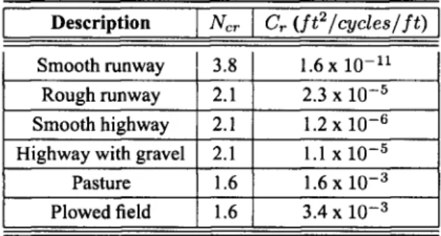
(37) Experiments. 21. For the present work, the algorithm to compute the APRBS signal was programmed in MATLAB™. In order to obtain a signal with normally distributed amplitude, the value of a was set to 0.01. In addition, the electric current values were bound between 0 and 2.5 A.. Stepped Increments Signal (SC) A SC signal is one in which the amplitude is held constant for a predetermined period of time. At the end of the period, the value of the signal is incremented to a different constant value. The purpose of the signal is to identify the various operational zones of the MR damper. In the present work, the electric current values were held constant for 30 seconds. Constant steps of 0.0, 0.4,0.8, 1.2, 1.6,2.1, and 2.5 A were employed.. 3.1.2. Displacement Pattern. As mentioned in [28], it is common to employ sine waves, step functions, or triangular waves as displacement patterns for vehicle testing. While these inputs provide a basis for comparative evaluation of various designs, they do not serve as a valid basis for studying the real ride behavior of a suspension system since surface profiles are rarely of simple forms. In consequence, it is found that road profiles are more realistically resembled by random functions. As discussed in [29] and [30], these random functions can be generally described by means of their frequency composition. According to the ISO 8606:1995 standard, there are eight different degrees of road roughness according to their power spectral density. Based on the work in [28], equation 3.3 describes the power spectral density of a road profile,. where S(f) represents the power spectral density of the elevation of the surface profile, / is a frequency in Hz, C. r. is the roughness coefficient of the road, ui is the number of cycles per feet, N x. cr. is a constant corresponding to the. roughness coefficient, and v is the speed at which the vehicle is traveling. c. Table 3.1 presents the values for C and N r. cr. depending on the desired road profile.. Table 3.1. Roughness coefficients for power spectral density functions of road profiles. Taken from [28].. Once a roughness coefficient has been selected, according to [30] the road profile x(t) can be generated based on a standard procedure as the sum of a series of harmonics. Equation 3.4 presents the calculation of a road profile,.

(38) 22. where <j>j is a random phase angle normally distributed in the interval 0 - 27r; ujj is a frequency within the interval at which S(f) is defined and calculated as Wj = w j m. Aw = (oj. max. - ui )/Nf; min. n. + Aw(j — 1); the frequency increment Aw is defined as. Nf is the total number of frequency increments in the interval uj. min. inside the square root represents the amplitude of the harmonics; w j and u) m. n. max. - w. m a x. ; the term. are the minimum and maximum. frequencies at which the spectrum is defined; and t represents the time. In the present work, road profile (RP) displacement patterns were chosen for all tests. The employed roughness coefficient was that of a smooth highway. The number of harmonics was selected as 100 with minimum and maximum frequencies of 0.2 and 20.5 Hz, respectively. The number of cycles per feet was set to 0.5 and the speed of the vehicle was selected as 440 in/s (25 mi/h). The values were employed in order to recreate the displacement pattern of a highway under standard conditions and contain a time-changing frequency with peak values around 6 Hz. In order to obtain the signals, the algorithm was programmed in MATLAB™. RP signals were employed in [31] to test passive suspension systems and in [10] to train ANNs in order to model the behavior of an MR damper.. 3.2. Experimental Setup. The selected experimental system can be divided into four parts: an MR damper, the actuators, the control system, and the data acquisition system. An ACDelco™MR damper, part of a Delphi MagneRide™ suspension from a Cadillac 2008, was employed. A n MTS™GT controller testing system was used to control the position of the damper. A Flextest™ data acquisition system commanded the controller and recorded the position and force of the MR damper, as well as the electric current on the coil. A sampling frequency of 512 Hz was used. The displacement actuator was a hydraulic servo-controlled piston of 3000 psi and displacement bandwidth of 15 Hz. The displacement and electric current ranges were: 0-1.6 in, and 0 - 2.5 A , respectively. The damping force was measured using an Instron load cell and the measured span was 0 - 640 lbf. The experimental setup was controlled and monitored by a Human-Machine Interface (HMI) developed in LabView™. A block diagram of the experimental setup is shown in Fig. 3.1.. 3.3. Signal Conditioning. 3.3.1. Noise Filter. The measured signals were observed to be highly permeated by noise. In order to remove the undesired noise frequencies, a filter was designed as a second order low-pass filter with a cutoff frequency of 20 Hz. Equation 3.5 presents the transfer function for the designed filter..

(39) Experiments. 23. Figure. 3.1. Block diagram of the experimental setup. The designed experiments are loaded as text files to the HMI. The HMI converts the files and sends the patterns to the control system. Then, a voltage respective to the desired position is sent to the actuation system, at the same time that the desired electric current is sent to the MR damper. The position, force, and temperature measurements are sent to the data acquisition system and are then passed to the HMI in the appropriate format. Finally, the HMI is in charge of formatting and saving the data.. 3.3.2. Discrete Derivative. In order to compute the velocity of the MR damper, a discrete-time derivative was employed after the displacement signal was filtered. The calculations were performed using Simulink (see appendix A).. 3.4. Experimental Results. Eight sets of experimental data were obtained for the identification of MR damper models. In the selected experiments, the electric current patterns were CS, ICPS, PRBS, and APRBS signals. On the other hand, RP patterns were employed as the displacement input. Three 30 s experiments were performed for the highly varying electric current patterns. In addition, two 600 s experiments with APRBS and ICPS electric current patterns were performed in order to test the behavior of the MR damper as the temperature of the device increased. Finally, three 210 s experiments were carried out employing SC electric current patterns. Various replicates of the experiments were performed and used as validation data. The specific patterns of the eight experiments are shown in Table 3.2, where the experiments have been labeled according to the patterns employed. The table specifies the utilized input patterns, the number of replicates performed, the duration of the experiments, the maximum displacement frequency, and the displacement span. Moreover, figures 3.2 and 3.3 show 20 and 100 second windows of the patterns employed for the first and last experiments, respectively. In addition, 30 and 60 second windows present the frequency content of the experiments. See Appendix A for a complete comparison of the experimental data sets .. 3.5. Summary. A description of the design of experiments, experimental setup, and resulting data sets was presented in this chapter. Various electric current patterns were selected in order to characterize the behavior of the MR damper. On the other hand, displacement patterns that resembled usual operating conditions of an automotive suspension system were chosen. The experimental setup and process were specifically described. At the end, eight experimental data sets were obtained in order to be used as training patterns for models of an industrial MR damper..

(40) 24. Table 3.2. Experimental data sets. Figure. 3.3. Description of experiment RP3-CS. Displacement and electric current patterns (left). Frequency content (right)..

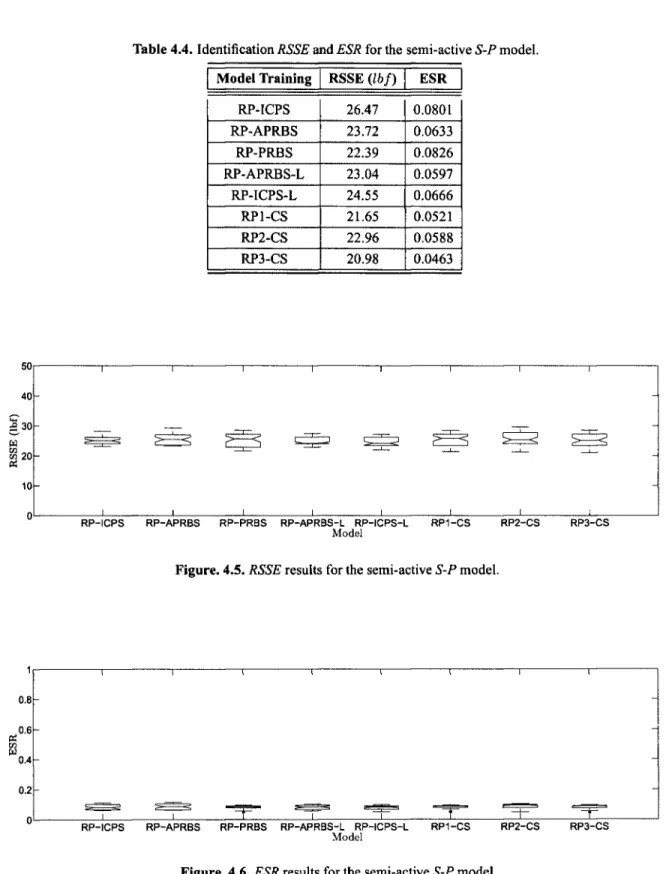
(41) Chapter 4. Results An extensive comparison of MR damper models is presented. The study is motivated on the challenge that involves the correct modeling of an MR damping system. Four models were selected among the state of the art, one from each modeling technique presented in the previous chapter. The models were trained using eight sets of experimental data and two error indexes were calculated. The results are presented by means of box-and-whisker diagram plots.. 4.1. Error Calculation. Among the state of the art, the selected models were the ones presented in [5], [32], a black-box model structure used in [10] and [33], and a fuzzy model that uses ANFIS as presented in [12] and [20]. The models were compared against each other by using the Square Root of the Sum of the Squared Errors (RSSE) and the Error to Signal Ratio (ESR) indexes. The RSSE and ESR are presented in equations 4.1 and 4.2, respectively. The RSSE presents the square root of the sum of the errors between the predicted and experimental output forces normalized by the total number of samples. The ESR is the ratio of the sum of squared errors and the variance of the experimental force. This last index is equal to one if the model is trivial and zero if the model is perfect.. The eight selected sets of experimental data discussed in the previous chapter were employed to train the structures. The models were identified using the first replicate of each experiment and cross validated with the remaining ones. The first three models were first identified in their passive form. This is, no electric current dependency was included. Then, the models were identified in their semi-active form. This is, the electric current was taken into account. The fuzzy-based structure was only identified in its semi-active form. At the end of the chapter, a non-linear fuzzy structure is proposed as an alternative for modeling an MR damper.. 25.

(42) 26. 4.2. ARX Model. The ARX structure shown in 2.8 was modified to consider three regressors for each input variable (x(t), x(t), F(t)) instead of two (see equation 4.3). Using the first replicate of each experiment, the nine coefficients of the model were identified with MATLAB™ using a nonlinear least squares algorithm. Then, the RSSE and ESR were calculated by comparing the experimental force with the force predicted by the models. The coefficients were randomly initialized 25 times and the lowest error value was recorded. The resulting identification errors are shown in Table 4.1. The identified coefficients for the different ARX structures can be seen in Appendix B .. Notice that for every ARX model identified, the RSSE and ESR lie below 12 lbf and 0.03, respectively even for the experiments with high electric current variations. In addition, a marked improvement can be seen for the models trained with the experiments that use constant steps of the electric current. Next, the eight identified models were validated using the remaining replicates and experiments. The resulting RSSE and ESR values by model are depicted in Figs. 4.1 and 4.2, respectively. The figures present a box and whisker plot with one box for each ARX model. The boxes have lines at the lower quartile, median, and upper quartile values. The whiskers are lines extending from each end of the boxes to show the extent of the rest of the data. Outliers are data with values beyond the ends of the whiskers. The models are named according to the experiments with which they were trained. From the figure, it can been seen that the models trained with the experimental data sets with constant electric current obtained various RSSE and ESR values over 20 lbf and 0.10, respectively. On the other hand, the ARX models identified with experiments that contain varying electric current can be observed to have less error values overall. In order to include the variant electric current in the model, the ARX structure was modified by adding three regressors. Equation 4.4 shows the final structure..

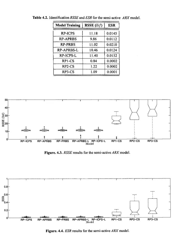
(43) Results. 27. RP-ICPS. RP-APRBS. RP-PRBS. RP-APRBS-L. RP-ICPS-L. RP1-CS. RP2-CS. RP3-CS. RP2-CS. RP3-CS. Model. Figure. 4.1. RSSE results for the passive ARX model. RP-ICPS. RP-APRBS. RP-PRBS. RP-APRBS-L. RP-ICPS-L. RP1-CS. Model. Figure. 4.2. ESR results for the passive ARX model. As for the passive model, the modified ARX semi-active model was trained using the first replicate of each of the eight sets of experimental data. As for the passive structure, 25 random initializations of the 12 coefficients were performed and the lowest error was recorded. The resulting identification errors are shown in Table 4.2. The identified coefficients for the different ARX structures can be seen in Appendix B. It should be noted that the addition of the three electric current regressors improved only slightly the performance of the ARX models. To further analyze the performance, the eight identified semi-active models were cross validated using the remaining replicates and experiments. The resulting RSSE and ESR values by model are depicted in Figs. 4.3 and 4.4, respectively. It can be observed that the results are nearly identical to the results obtained with the passive ARX model for the first five models. Nonetheless, for the models trained with experiments that held the electric current constant, the validation results were not satisfactory..