Departamento de Análisis Económico y Administración de
Empresas
Facultad de Economía y Empresa
Universidade da Coruña
Three Essays in Regional Economics:
The Case of Romania
TESIS DOCTORAL PRESENTADA POR:
Cosmin Gabriel Bolea
DIRIGIDA POR:
Dr. Jesús López-Rodríguez
Universidade da Coruña
Contents
Acknowledgments 11
Abstract 13
Resumen 13
Resumo 14
I. Introducción 15
II. Metodología: Marco Teórico 18
III. Metodología: Estimación Empírica 20
Chapter 1: Economic Remoteness and Wage Disparities in Romania 23
1.1. Introduction 25
1.2. Theoretical Framework 30
1.3. Econometric Specification 35
1.4. Data Source and Construction of variables 36
1.5. Empirical Results 38
1.5.1. Market Access and Wages: Preliminary Analysis 38 1.5.2. Baseline Estimations: OLS Estimations 42
A. Instrumental Variables 44
B. Robustness Checks 47
C. Spatial Dimension 53
1.6 . Final Remarks and Conclusions 56
Chapter 2: Economic Geography, Human Capital and Policy
Implications in Romanian counties 59
2.1. Introduction 61
2.4. Empirical Analysis 73 2.5. Conclusions and Some Policy Implications 93
Chapter 3: Growth dynamics and Transition in the Romanian Economy:
1995-2008 99
3.1. Introduction 101
3.2. The Neo-Classical Model of Growth and the Convergence
Hypothesis 103
3.2.1. The Neo-Classical Model of Growth 103 3.2.2. Convergence in the Neo-Classical Model of Growth 105
3.2.2.1. Theoretical concept 105
3.2.3. Methodologies of Convergence Analysis 108 3.2.3.1. Cross Section estimation of absolute convergence 108 3.2.3.2. Cross Section estimation of conditional convergence 109 3.2.3.3. Panel data estimation of convergence 110
3.2.3.4. Markov Chain Models 111
3.3. A brief overview of the transition process in Romania: Some
Important facts 113
3.3.1. Economy 117
3.3.2. Demography 119
3.3.3. Health care system 119
3.3.4. Education system 120
3.5. Regional growth in Romania by typology of region: 1995-2008 146 3.6. Growth dynamics and Economic Geography in Romania: 1995-2008 160
3.7. Principal Component Analysis 165
3.8. Conclusions 175
Conclusions and Contributions of the Thesis 179
References 185
Annexes 195
A. Appendix to chapter 1: 197
Figures
Figure 1.1: GDPpc and Distance from Timisoara (Romania 2006) ... 27
Figure 1.2: Wages and Market Access (Romania, 2006) ... 38
Figure 1.3: Wages and Domestic Market Access (Romania, 2006) ... 41
Figure 1.4: Wages and Foreign Market Access (Romania, 2006) ... 41
Figure 1.5: GDP per capita and Domestic Market Access (Romania, 2006) ... 42
Figure 1.6: Secondary and Tertiary Education and Market Access (Romania, 2006) ... 48
Figure 1.7: Primary Education and Market Access (Romania, 2006) ... 49
Figure 1.8: R&D Expenditure and Market Access (Romania, 2006) ... 49
Figure 1.9: Moran scatterplot for the log of Wages in 2006 ... 55
Figure 2.1: Higher Education and Distance from Timisoara (Romania, 2006) ... 75
Figure 2.2: Secondary and Tertiary Education and Market Access (Romania, 2006) ... 76
Figure 2.3: Primary Education and Market Access (Romania, 2006) ... 77
Figure 2.4: Cesar Bolliac´s map of 1853 Comercial Routes in Romania ... 89
Figure 3.1: Average Growth Rate in Romania by periods: 1995-2008 ... 127
Figure 3.2: Average Growth Rate in Romania by periods: 1995-2008 ... 130
Figure 3.3: Average Growth Rate in Romania by periods: 1995-2000 ... 132
Figure 3.4: Average Growth Rate in Romania by periods: 2000-2004 ... 133
Figure 3.5: Average Growth Rate in Romania by periods: 2004-2008 ... 135
Figure 3.6: Average Growth Rate in Romania by periods: 2000-2008 ... 136
Figure 3.7: Average Growth Rate in Romanian counties: 2000-2008 .... 139
Figure 3.8: Average Growth Rate in Romanian counties: 1995-2000 .... 142
Figure 3.9: Average Growth Rate in Romanian counties: 2000-2004 .... 143
Figure 3.11: Average Growth Rate in Romanian counties: 2000-2008 .. 145 Figure 3.12: Growth performance of Romanian counties: 1995-2008 (variables nationally standardized) ... 149 Figure 3.13: Growth performance of Romanian counties: 1995-2000 (variables nationally standardized) ... 152 Figure 3.14: Growth performance of Romanian counties: 2000-2004 (variables nationally standardized) ... 154 Figure 3.15: Growth performance of Romanian counties: 2004-2008 (variables nationally standardized) ... 157
Maps
Map 1.1: GDP per Capita in Romanian Regions ... 27 Map 1.2: Spatial percentile distribution for the log of Wages in 2006, (LnAMEG) ... 54 Map 3.1: Real GDP per capita growth rate in Romanian economic regions 1995-2008 ... 130 Map 3.2: Real GDP per capita growth rate in Romanian economic regions 1995-2000 ... 132 Map 3.3: Real GDP per capita growth rate in Romanian economic regions 2000-2004 ... 134 Map 3.4: Real GDP per capita growth rate in Romanian economic regions 2004-2008 ... 135 Map 3.5: Real GDP per capita growth rate in Romanian economic regions 2000-2008 ... 136 Map 3.6: Real GDP per capita growth rate in Romanian economic regions 1995-2008 ... 140 Map 3.7: Growth rate in Romanian economic regions 1995-2008
Map 3.9: Growth rate in Romanian economic regions 2000-2008 ... 145
Map 3.10: Growth rate in Romanian economic regions 2000-2008 (average=100) ... 146
Map 3.11: Growth rate in Romanian economic regions 1995-2008 ... 150
Map 3.12: Growth rate in Romanian economic regions 1995-2000 ... 153
Map 3.13: Growth rate in Romanian economic regions 2000-2004 ... 155
Map 3.14: Growth rate in Romanian economic regions 2004-2008 ... 158
Map 3.15: Growth performance of Romanian economic regions 2000-2008 ... 160
Tables
Table 1.1: GDPpc and Gross Wages: Romania (2006) ... 26Table 1.2: Summary Statistics on Market Access: Romania (2006) ... 39
Table 1.3: Market Access and Romanian Income: Baseline Estimations (Romanian Regions, 2006) ... 43
Table 1.4: Market Access, Human Capital and R&D Expenditure (Romanian regions, 2006) ... 50
Table 1.5: Market Access and Regional Income: Extended Estimations (Romanian Regions, 2006) ... 51
Table 2.1: Educational Attainment Levels in Romania (2006) ... 74
Table 2.2: Market Access and Educational Levels: Baseline Estimations (Romania, 2006) ... 78
Table 2.3: Market Access, Regional Dummies, Educational Levels and Average Years of Education ... 84
Table 2.4: Romanian Higher Education as a function of market access: TSLS instrumental variable regression (2006) ... 90
Table 3.2: Average growth rate by regions and periods ... 138
Table 3.3: Classification of Romanian counties: 1995-2008 ... 151
Table 3.4: Classification of Romanian counties: 1996-2000 ... 153
Table 3.5: Classification of Romanian counties: 2001-2004 ... 156
Table 3.6: Classification of Romanian counties: 2005-2008 ... 158
Table 3.7: Regional Growth estimations ... 164
Table 3.8: Total Variance Explained, 1995 ... 168
Table 3.9: Rotated component Matrix, 1995 ... 169
Table 3.10: Total Variance Explained, 2000 ... 170
Table 3.11: Rotated component Matrix, 2000 ... 171
Table 3.12: Total Variance Explained, 2008 ... 173
Acknowledgments
During these years, there are many people and institutions that have participated in this work. To all of them I want to express my gratitude for the support and confidence they have given to me so selflessly. I would like firstly to thank the Department of Economic Analysis and Business Administration at the University of A Coruña for giving me the opportunity to complete my graduate studies. I especially want to acknowledge the great debt I have with my supervisor, teacher and friend Jesus Lopez-Rodriguez. He is the one who put me in the right way for the realization of this PhD thesis despite the inconsistency of my first research proposal. To him, I must first thank the path, the indications and the aid to develop this thesis. Thanks for the conviction that you showed me when the uncertainty didn’t allow me to glimpse the horizon. I consider myself a privileged person to have your friendship and supervision during this research. His academic expertise has given me the resolution of the difficulties encountered in the course of the investigation. Thank you also for your great generosity in the effort you have shown to me during these five years we have worked together sacrificing some of your free time to make this project go ahead and made me feel at home even if I was far away from it. Therefore I will permanently be in debt with you Jesús.
I also appreciate the lessons and support from my teachers and very especially from Andres Faiña, Miguel Marquez-Paniagua and Atilano Pena López for their time devoted to help me out to solve the problems that often occur running econometric programs. A special thanks goes to Domingo Calvo Dopico for all the time devoted to discuss and help to disentangle the results coming from the Principal Component Analysis in the last chapter of the thesis
and Business at the University of A Coruña between 18-23 of January 2012.
We also thank the comments and suggestions received from David Brasington, Sandy Dall´erba, David Plane, Alexandru Jivan, Geoff Hewings, David Gibson and other participants during the presentations of the various chapters of this thesis carried out by my supervisor at the University of Cincinnati, University of Arizona, the Regional Economics Applications Laboratory (REAL) at University of Illinois at Urbana Champaign, the Institute of Capital, Creativity and Innovation (IC2) at the University of Texas, The Real Colegio Complutense (RCC) at Harvard and at the West University of Timisoara.
Finally thanks to all who showed interest and participated in the presentation of the various chapters of this thesis in the VI World conference of the Spatial Econometrics Association (Salvador, 2012), Southern Regional Science Association (Charlotte, 2012) Simposio of Economic Analysis (Malaga, 2011), Scientific Symposium: Global Crisis and the Reconstruction of the Economic Science, Faculty of Economics, Economic Studies Academy (Bucharest, 2011), Spanish Regional Science Conference (Badajoz, 2010); 5th International ´conference on Applied Statistics organized by the National Institute of Statistics and Academy of Economic Studies (Bucharest, 2010); 5th Annual International Symposium on Economic Theory, Policy and Applications (Athens, 2010). Thank you to Paulino Montes-Solla without whom this thesis would not have had this rigorous and formal appearance. I also thank Aaron Parada, a research assistant during 2012 at the Department of Economic Analysis and Business Administration for their excellent support during the preparation of Chapter 3 of this thesis.
To the friends of Spain, Mexico and Brazil and of course those of Romania that patiently waited for this moment to come and that despite the distance they were always by my side.
All this work would never have been possible without the unconditional support of my family, my parents, my grandparents and my brothers, and especially without the love of Esperanza Luciano Fonseca.
Abstract
Chapter 1 derives an econometric specification which relates the income levels of a particular location with a weighted sum of the volume of economic activities of the surrounding locations (market access). Then, empirically, we estimate this econometric specification for a sample of 42 Romanian regions in the year 2006. The results show that market access is statistically significant and quantitatively important in explaining cross-county variation in Romanian per capita GDP levels. Chapter 2 looks at the link between human capital and geographical location in Romania. The results show that the percentage of individuals with medium and high educational levels is affected positively by the regions´ market access even after looking for third variables that might be affecting regional educational levels and which work through accumulation incentives.
Chapter 3 focuses on the analysis of the growth dynamics in the Romanian economic over the period 1995-2008 and the link between them and the economic geography of the country. The results of our analysis point out that a catching-up process across Romanian counties is not taken place and that the economic geography of the country is shaping the growth dynamics observed over the course of the years analyzed in this chapter.
Resumen
El capítulo 1 deriva una especificación econométrica que relaciona los niveles de renta en una localización con una media ponderada por la distancia del volumen de actividad económica de las localizaciones colindantes (market access en su denominación anglosajona). Empíricamente, se estima esta especificación econométrica para la muestra de las 42 regiones rumanas en el año 2006. Los resultados demuestran que el market access es estadísticamente significativo y cuantitativamente importante a la hora de explicar las diferencias regionales en los niveles de PIB per cápita en Rumanía.
del market access de las regiones incluso después de controlar por otras variables que pueden influir en los niveles educativos.
El capítulo 3 se centra en el análisis de la dinámica de crecimiento de las regiones rumanas en el período 1995-2008 y en el link entre esta dinámica y la geografía económica del país. Los resultados del análisis muestran que no existe un proceso de convergencia entre las regiones rumanas y por otro lado que la geografía económica del país tiene un efecto importante a la hora de explicar la dinámica de crecimiento observada en el período analizado en este capítulo.
Resumo
O capítulo 1 deriva unha especificación econométrica que relaciona os niveis de renda nunha localización con unha media ponderada pola distancia do volume de actividade económica nas localizacións lindantes (market access na súa denominación anglosaxona). Empiricamente, estimase esta especificación econométrica para a mostra das 42 rexións romanesas no ano 2006. Os resultados demostran que o market access e estatisticamente significativo e cuantitativamente importante a hora de explicar as diferenzas rexionais nos niveis de renda per cápita en Romanía.
O capítulo 2 analiza a relación entre capital humano e localización xeográfica en Romanía. Os resultados mostran que o porcentaxe de individuos con niveis educativos medios e altos depende positivamente do market access das rexións incluso despois de controlar por outras variables que poden influír nos niveis educativos.
I.
Introducción
El objetivo de la presente tesis doctoral es triple: a) Analizar en que medida la ecuación nominal de salarios que constituye una de las ecuaciones estructurales mas importantes en términos de aplicabilidad empírica de los modelos centro-periferia de Nueva Geografía Económica se verifica en el caso de las disparidades observadas en los niveles de renta entre las diferentes regiones (condados) rumanas, b) Analizar en que medida las predicciones teóricas mas recientes de los modelos centro-periferia de Nueva Geografía Económica que vinculan la localización geográfica con la acumulación de capital humano se verifican para el caso de Rumanía y c) analizar en que medida los patrones de crecimiento regional observados en las regiones rumanas pueden vincularse a la geografía económica del país.
que el ratio entre el PIB per cápita de la región más rica (Bucharest) y la media del país es superior a 5. Incluso excluyendo de los cálculos la capital del país el ratio es superior a 3. Si hacemos la comparación entre la región mas rica y la mas pobre el ratio se dispara a 18.30 (incluyendo Bucharest) y 9.59 respectivamente (sin Bucharest), b) Los niveles de desarrollo en Rumania muestran un fuerte patrón centro-periferia. La distribución espacial de los niveles de renta en Rumanía muestra que lo que en el lenguaje de los modelos de Nueva Geografía Económica se denomina centro estaría representado principalmente por las regiones del oeste y noroeste del país mientras que la periferia estaría representada por las regiones del noreste y sureste. Otra forma alternativa de ver este patrón centro-periferia es mediante un gráfico que recoja la relación entre el PIB per cápita de cada una de las regiones y su distancia a Timisoara (ciudad localizada en el oeste del país). Los datos reflejan que a medida que nos movemos cada vez más lejos de Timisoara el nivel de renta de las regiones es cada vez menor.
Craiova que es donde se localizan las universidades mas importantes del país. Si comparamos los datos de la educación secundaria en estas regiones con la media del país se ve que los resultados están bastante por encima de la media. En el otro extremo, las regiones rumanas que están localizadas lejos de esto polos de crecimiento, en lo que podría denominarse la periferia económica Neamţ, Mureş, Tulcea, Satu Mare, Botosani, Vaslui, Olt, Teleorman tienen cifras de educación superior por debajo de la media del país. Además, en la distribución espacial de los niveles de capital humano se muestra también un fuerte gradiente centro-periferia que se puede observar fácilmente en un gráfico relacionando los niveles de educación superior con la distancia a Timisoara. Los datos muestran que cuando más lejos nos encontremos de Timiosara menores serán los niveles de educación secundaria y terciaria.
II. Metodología: Marco Teórico
El marco teórico para el análisis realizado a lo largo de esta tesis doctoral se basa por un lado en el uso de modelos de Nueva Geografía Económica (capítulo 1 y 2) y por otro en los modelos neoclásicos de crecimiento económico (capítulo 3).
En relación a los capítulos 1 y 2 existen muchos elementos que pueden justificar el porque los niveles de desarrollo o los niveles de capital humano varían de unas regiones a otras. Desde el punto de vista de las teorías del crecimiento económico (Barro and Sala-i-Martin, 1991, 1995) muestran que diferencias en los niveles de ahorro, niveles de inversión, gasto en I+D, dificultades en la transmisión de tecnología etc. pueden explicar por qué las regiones no converjan. Las teorías tradicionales de desarrollo económico por otro lado ponen más énfasis en los factores de geografía de primera naturaleza (geografía física) que en los factores de segunda naturaleza (geografía económica). Factores como acceso a ríos navegables, puertos, aeropuertos, recursos naturales, horas de sol, etc. estarían en la base de estos modelos (véase Hall and Jones, 1999). Dentro de las teorías de la economía urbana se enfatizan factores como las economías externas de escala que surgen de poner los recursos relevantes en proximidad espacial, por ejemplo en la misma ciudad, lo cual aumentaría la productividad de las empresas y de los trabajadores (Marshall, 1920; Henderson, 1986; Duranton and Puga, 2004).
modelos de equilibrio general con fundamentación microeconómica y a diferencia de las teorías de crecimiento económico tienen en cuenta los aspectos geográficos, concretamente los aspectos de geografía económica y por tanto la estructura geográfica de la producción, niveles de renta y capital humano puede ser analizada explícitamente.
En el capítulo 3 metodológicamente nos centramos en la literatura empírica que se deriva de los modelos de crecimiento neoclásico (Barro and Sala-i-Martin, 1991, 1995) pero incorporamos a nuestro análisis componentes de geografía económica para ver en que medida éstos están en la base de los distintos patrones de crecimiento observados en el período analizado en esta tesis doctoral.
distintas regiones.
III. Metodología: Estimación Empírica
En relación a la estimación empírica de los diferentes modelos propuestos, en el capítulo 1 se estima econométricamente la relación entre los niveles de renta en el año 2006 para las 42 regiones rumanas (condados) y nuestra variable clave de geografía económica que es el market access. Se completa este modelo de base con; a) un modelo ampliado donde se recogen diferentes variables de control para desenredar el efecto que el market access tiene en los niveles de renta y b) un modelo espacial para controlar por los posibles problemas de autocorrelación espacial. Las estimaciones se realizan por mínimos cuadrados ordinarios (MCO) y también se recurre a la estimación mediante el uso de variables instrumentales para controlar por los posibles problemas de endogeneidad entre el market access y nuestra variable dependiente.
las regiones y por otro mediante la ordenación de los niveles educativos en bajos, medios y altos y estimando un modelo probit ordenado. Las estimaciones las realizamos mediante mínimos cuadrados ordinarios (MCO) y también mediante el uso de variables instrumentales para controlar por los posibles problemas de endogeneidad. El capítulo contiene un análisis muy extensivo mediante el uso de diferentes instrumentos basados en la literatura reciente de la Nueva Geografía Económica (Combes et al., 2010).
Chapter 1: Economic Remoteness and Wage Disparities
in Romania
1Abstract
This chapter looks at the link between per capita GDP disparities and market access for the Romanian regions. In first place, we derive an econometric specification which relates the income levels of a particular location with a weighted sum of the volume of economic activities of the surrounding locations (market access). Then, empirically, we estimate this econometric specification for a sample of 42 Romanian regions in the year 2006. The results show that market access is statistically significant and quantitatively important in explaining cross-county variation in Romanian per capita GDP levels. Moreover, our results are robust to the inclusion of control variables thought to be important in explaining Romanian income levels as it is the case with human capital and innovation levels. After controlling for these variables, market access remains still positive and statistically significant although its influence on per capita GDP levels decreases around 25%. Finally some policy conclusions are also drawn.
Key Words: Economic Remoteness, Market Access, Wage Disparities, Romania
JEL Classification: R11, R12, R13, R14, F12, F23
1 A version of this chapter has been published as : Lopez-Rodríguez, J., Faiña A. and C. Bolea-Gabriel
1.1. Introduction
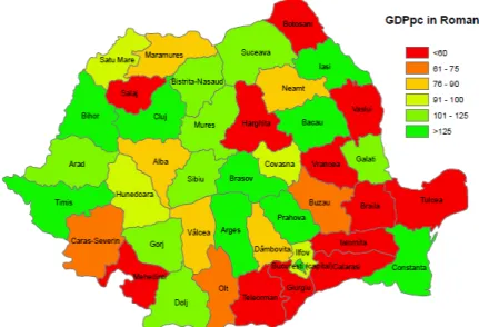
The favourable evolution of the Romanian economy in recent years and especially after its take off in 2004 has allowed an important improvement of the development levels among its regions although this development was quite uneven. The Romanian accession to the European Union (EU) meant that it has had to reorganize its territory in order to have a more efficient EU fund absorption. From the 42 existing counties, Romania has created 8 economic regions2 although without legal personality. The counties belonging to the Northeast (1) and Southeast Economic Regions (2) are far removed from the main European markets and experience severe underdevelopment problems. Moreover, their sectoral structure is heavily based on agriculture. On the other hand, the counties belonging to the West (5), Northwest (6) and Center (7) Economic regions benefit from a better location with respect to the main European markets having more potential to attract investors. Table 1 shows the values of Gross Domestic Product per capita (GDPpc) for the 42 Romanian counties in 2006. The results show quite clearly the dominance of the nation's capital (Bucharest). Per capita GDP in Romania is more than five times higher than the national average. Comparing Bucharest with the poorest county (Giurgiu) the data show overwhelming differences (per capita GDPpc in Bucharest is more than 18 times higher than that of Giurgiu.
If we exclude from the calculations the distortion generated by the capital values, the results still show that in Romania there is a strong regional contrast in terms of per capita GDP. Thus, table 1.1 shows that
2 We are going to use the word/s region/s throughout the chapters of this thesis which are more
the richest city after Bucharest, Timisoara, has a per capita GDP which is over three times higher than the national average.
Table 1.1: GDPpc and Gross Wages: Romania (2006)
County GDPpc County GDPpc
Constanţa 2715 Bistriţa-Năsaud 1820
Galaţi 1848 Cluj 3050
Tulcea 690 Maramures 1440
Vrancea 954 Satu Mare 1670
Arges 2723 Salaj 735
Călăraşi 653 Alba 1350
Dambovita 1560 Braşov 2718
Giurgiu 589 Covasna 1590
Ialomita 840 Harghita 1037
Prahova 3040 Mureş 2154
Teleorman 974 Sibiu 1801
Dolj 1850 Ilfov 1671
Gorj 2000 Bucureşti 10780
Calculation including the capital
(Bucharest) Calculation without the capital (Bucharest)
Average 1948 Average 1691
Max. 10780 Max. 5651
Min 589 Min 589
Ratio max./med 5.53 Ratio max./med 3.34
Ratio max./min. 18.30 Ratio max./min. 9.59 Source: Own elaboration based on INSSE figures
alternative way of looking at the “center-periphery” gradient in Romania is by plotting GDPpc against distance to Timisoara (Figure 1.1). The results show that as we move further away from Timisoara, per capita GDP figures (on average) decreases.
Map 1.1: GDP per Capita in Romanian Regions
(Index, Average 2006 GDPpc Romania=100) Source: Own elaboration based on INSSE figures
Figure 1.1: GDPpc and Distance from Timisoara (Romania 2006)
y = -0,001x + 7,879
Distancia from Timisoara (Km)
At a theoretical level there are many factors that explain why different regions within a territory do not converge. From the standpoint of economic growth theories (Barro and Sala-i-Martin, 1991, 1995) show that differences in savings rates, investment rates, skilled human capital and difficulties in technology transmission could explain this lack of convergence. Traditional theories of economic development put more emphasis on first nature geography factors, i.e. the natural advantages of different locations (access to navigable rivers, ports, airports, allocation of oil, hours of sunshine, etc.) (See Hall and Jones, 1999). Urban economics theories emphasize the external economies of scale that arise from placing relevant resources in spatial proximity, for instance in the same city, which improves productivity of firms and workers in local environments (Marshall, 1920; Henderson, 1986; Duranton and Puga, 2004).
empirical level, Krugman (1991) model has triggered a plethora of contributions for different geographical scenarios: On the one hand it can be mentioned the contributions looking at income differences for cross country samples or cross regional samples involving different countries (Redding and Venables, 2004; Breinlich, 2006; Head and Mayer, 2006; and Lopez-Rodriguez and Faiña, 2007, and Lopez-Rodriguez et al. 2011). On the other hand, there are the contributions looking at cross regional income differences carried out at single country level (Hanson, 2005; Roos, 2001; De Bruyne, 2003; Mion, 2004; Pires, 2006). However, to the best of our knowledge, there are no studies at country level of the forces put at work in Krugman´s (1991) model for any Central and Eastern European country.
to reduce transport costs directly via improvements in infrastructure (e.g. roads, ports, etc.) which in the case of Romania are still very much lagging behind.
The remaining part of the chapter is structured as follows: Section 2 introduces the theoretical framework from which the econometric specifications are derived and are used in the subsequent sections. Section 3 contains the econometric specifications which will be estimated using Romanian data. Section 4 provides information about data sources and the main variables of our analysis. Section 5 presents the results of the estimations and finally, section 6 contains a summary of the main contributions of the chapter and draws some policy conclusions.
1.2. Theoretical Framework
Our theoretical framework is a reduced form of a standard New Economic Geography model 3 (multiregional version of Krugman (1991) model) which incorporates the key ingredients to obtain the so called nominal wage equation which will constitute the workhorse of our empirical estimation.
We consider a world with R regions
(
j
=
1
,
2
,
,
R
)
, and we focus onthe manufacturing sector, composed of firms that produce a great number of varieties of a differentiated good
( )
M
under increasingreturns to scale and monopolistic competition. Transportation costs of differentiated goods are in the form of iceberg costs so in order to receive 1 unit of the differentiated good in location j from location i,
Ti,j >1 units must be shipped, so Ti,j =1 means that the trade is
costless, while Ti,j−1 measures the proportion of output lost in shipping from i to
j
. The manufacturing sector can produce in differentlocations
On the demand side, the final consumers´ demand in location
j
can beobtained by the utility maximization of the following CES function:
j
Where
M
j represents the consumption of the differentiated good in locationj
. D is an aggregate of the different industrial varieties definedby a CES function à la Dixit and Stiglitz (1977):
1
produced on location i,
σ
is the elasticity of substitution between anytwo varieties where
σ
>1. If varieties are homogenous,σ
goes to infinite and if varieties are very different,σ
takes a value close to 1. Consumers maximize their utility (function 1.1) subject the following budget constraint:where pij (pij = piTij), is the price of varieties produce at location i
(for the derivation and discussion of this equation, we refer to appendix A to chapter 1).
This Industrial Price Index of location j measures the minimum cost of
buying 1 unit of the differentiated good M so it can be interpreted as an
expenditure function. If we rewrite the expenditure on consumption as j
Turning to the supply side, a representative country firm maximizes the following profit function:
The technology of the increasing returns to scale sector is given by the usual linear cost function:
l
Mij= +
F
cx
ijM,
where lMij represents theindustrial labour force needed to manufacture 1 unit at location i and
sell it at location
j
, F are the fixed costs units which are needed formanufacturing the industrial good,
c
is the unit variable cost andx
ijM is the quantity of each variety demanded at locationj
and produced atlocation i ( iM ijM
j
firm at location i and sold at different
j
locations) and wiM is thenominal wage paid to the manufacturing sector workers at location i.
Increasing returns to scale, consumers´ love of variety and the existence of a limited number of potential varieties of the manufacturing good mean that each variety is going to be produced by a single firm at single location. In this way, the number of manufacturing firms coincides with the number of varieties. Each firm maximizes is own profit behaving as a monopolist of its own variety of the differentiated good. First order conditions for profit maximization lead us to the standard result that prices are a mark-up over marginal costs.
1
σ represents the Marshall-Lerner Price-cost ratio. The higher
the ratio, the higher the monopolistic power of the firm. Krugman (1991) interprets σ as an inverse measure of the scale economies due to its interpretation as a direct measure of the price distortion and as an indirect measure of the market distortion due to the monopoly power. Since
1
−
σ
σ is higher than 1, Krugman (1991) interprets this result as a
proof of increasing returns to scale. Substituting this pricing rule into the profit function, we obtain the following expression for the equilibrium profit function:
( 1)
The price needed to sell this many units is given by
∑
σ
. Combining this expression with the fact that
prices are a constant mark-up over marginal costs in equilibrium,
we obtain the following zero-profit condition:
1
This equation is called nominal wage equation which constitutes the key relationship to be tested in the empirical part of this work. According to equation (10), the nominal wage level in each location depends on a weighted sum of the purchasing capacities of the different locations where the weighted scheme is a decreasing function of the distance between locations. In the New Economic Geography literature, the expression on the right hand side of equation (1.10) has been labelled with different names market access (Redding and Venables, 2004) and real market potential (see Head and Mayer, 2004)4.
We will refer to this expression as market access and will be labelled as MA. The meaning of this equation is that access advantages raise local factor prices. More precisely, production sites with good access to major markets because of its relatively low trade costs tend to reward their production factors with higher wages.
4 This expression is semantically analogous to the one employed by Harris (1954) but the term real
If we normalize the way we measure production, choosing the units such
F , and defining the market access of location i
as 1 1
=
∑
, we can rewrite the nominal wage equation as:1 M
w MA
i = i σ
(1.11)
This simplification of the nominal wage equation is very similar to the Harris (1954) market potential function in the sense that economic activity is more important in those regions which are close to large markets.1.3. Econometric Specification
Taking logarithms in expression (1.11), the estimated nominal wage equation expressed in per capita terms is based on the estimation of the following expression:
However equation (1.12) is a restricted specification to analyze the potential effects market access has on wages as we cannot say whether the regression captures causality or simply captures correlations with omitted variables such as human capital, innovation and so on. To address these potential impacts and control for the possibility of other shocks that are affecting the dependent variable and are correlated with market access, we also estimate an alternative specification that explicitly takes into account the above considerations. Therefore we expand our baseline estimation (eq. 1.12) to allow for the inclusion of control variables which may be affecting cross-county wage levels by estimating the following equation:
1.4. Data Source and Construction of variables
The data for this chapter refers to the year 2006 and was taken from different sources, National Statistical Institute of Romania (INSEE), the statistical office of the European Union (EUROSTAT) and data from various ministries of the Romanian Government.
First, the dependent variable of the model was approximated by using 2006 data on per capita GDP at county level. These data come from the Romanian National Statistical Institute.
surrounding regions. We proxy each county´s volume of economic activity by its total gross domestic product. With respect to the calculation of the discount factor (distance between regions) it is based on the distances measured in Km between the capital cities of the 42 counties in which Romania is divided. Data on distances between capital cities was obtained from the website www.travelworld.ro. The calculation of the internal distance within each county is approximated by a function that is proportional to the square root of each county´s area. The expression used for calculation is
π
Area 66 .
0 where "Area" represents the size of the county expressed in km2. This expression gives the average distance between two points on a circular location (see Head and Mayer, 2000; Nitsch, 2000; and Crozet, 2004; for a discussion of this measure of internal distance).
1.5. Empirical Results
1.5.1. Market Access and Wages: Preliminary Analysis
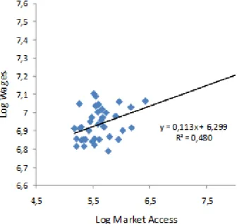
In this section we present and discuss a series of graphs which give a first visual approach to the empirical estimates carried out in the next section. Figure 1.2 plots log regional per capita GDP levels on log market access. This preliminary approach shows a positive effect of market access shaping regional per capita GDP levels which is in line with the theoretical propositions derived from the model proposed in section 2 of the chapter.
Figure 1.2: Wages and Market Access (Romania, 2006)
Source: Own elaboration based on INSSE figures
(FMA) of a Romanian county is the contribution made to total market access (TMA) by the surrounding Romanian counties. Therefore, the analysis of these two components of the TMA allows us to clarify the relative importance of each market access component and therefore we can estimate which has more impact in shaping per capita GDP at county level. Table 1.2 provides some information on the average composition of market access for the 42 Romanian counties by breaking down total market access (TMA) into its two components, the domestic component (DMA) and the foreign component (FMA).
Table 1.2: Summary Statistics on Market Access: Romania (2006)
County DMA TMA DMP/ TMA County DMP FMP DMP/ TMA
the Romanian most dynamic counties with percentages over total market access above 20% such as the cases of Iasi, Constanta, Timis, Cluj, Bihor and Bacau. Within this set of regions Iaşi county, located in the so-called Region 1-Northeast, and Timis county, Region 5-West, stand over the others with a domestic contribution to total market access above 40%. The reason behind these high values of the domestic component lies in the fact that these counties are important growth poles within the country with an important weight in both population and GDP. Timiş county, geographically situated in the west on the border with Serbia and Hungary, has a better access than other Romanian counties to the main central European markets. In fact within a 500 km radius there are four European capitals. Moreover, the county belongs to the euro-region DKMT (Danube, Cris, Mures-Tisa) jointly with other counties from Serbia and Hungary. The other case is Iasi, Romanian's most populous county with nearly 800,000 inhabitants, the ancient capital of the country (before unification) and the largest cultural center of eastern Romania. It works as a growth pole in the Region 1- Northeast. Cluj-Napoca is also an important pole of economic growth in Region 6-North West with a history marked by multiculturalism, along with the Region 7-Center, and the domination of the Austro-Hungarian Empire. These facts have made possible that Hungarian, German and Austrian investments in these regions are higher than the national average. Representative sectors in these counties are the pharmaceutical, the chemical and the high tech ones.
in each county but the important weight the domestic component of market access has in explaining income levels is clearly seen by the better fit of the regression.
Figure 1.3: Wages and Domestic Market Access (Romania, 2006)
Source: Own elaboration based on INSSE figures
Figure 1.4: Wages and Foreign Market Access (Romania, 2006)
The above figures show a positive relationship between income levels, per capita GDP figures and market access for the Romanian regions. The rationale behind these effects of market access on income levels is based on the direct trade cost savings that accrue to central locations.
Figure 1.5: GDP per capita and Domestic Market Access (Romania, 2006)
Source: Own elaboration based on INSSE figures
The above figures show a positive relationship between income levels, either approximated by wages or per capita GDP figures, and market access for the Romanian regions. The rationale behind these effects of market access on income levels is based on the direct trade cost savings that accrue to central locations.
1.5.2. Baseline Estimations: OLS Estimations
Table 1.3: Market Access and Romanian Income: Baseline Estimations (Romanian Regions, 2006)
Dependent Variable Log Wages 2006
Regressors (1) (2) (3) (4) (5) (6)
First Stage (t-statistic) 8.60 3.51 /8.29(size) 3.29(av.d)
Hansen J Statistic identified Exactly identified Exactly 3.11
R2 0.48 0.47 0.40 0.20 0.47 0.48
Prob (F-statistic) 0.00 0.00 0.00 0.00 0.00 0.00
Number observations 42 42 42 42 42 42 Note: Table displays coefficients and Huber-White heterocedasticity robust standard errors in parenthesis;** denotes statistical significance at 5% level ,* denotes statistical significance at 10% level; “First stage” R2 is the R2 from regressing market access on the instruments set, Instruments: region Size Column (2), Average Distance (5) and Average Distance and region Size (6)
Source: Own elaboration
The estimated coefficient on market access is positive and statistically significant at 5% level and the R2 of the regression is 0.48. This first result is in line with the theoretical expectations, showing that doubling a county market access would increase its income by 11%. As a robustness test, column (3) enters log domestic market access5 and column (5) enters log foreign market access6 as separate terms in the regression
5 The Domestic Market Access (DMA) of a region “i” refers to the contribution made to total market
access (MA) by the region itself.
6 The Foreign Market Access (FMA) of a region “i” refers to the contribution made to total market
equation. Theory tells us that this regression is misspecified, and we see that the R2 is lower than with the correct specification (column (1)). However, both terms are positively signed and statistically significant at the 5% level.
However, the use of market access as the only regressor brings the problem of reverse causality in the sense that in its computation we include the Gross Domestic Product of each Romanian county which in turn is increasing in per capita GDP as captured by the dependent variable, log per capita GDP. This endogeneity problem can cause inconsistent and biased estimates. In order to address this issue, we use instrumental variables to estimate the effect of market access on income levels.
A. Instrumental Variables
county’s size expressed in km2. This instrument captures the advantage of large regional markets in the composition of the domestic component of market access. In column 5 we instrument market access with the average distance of each county to the surrounding ones. This instrument captures the market access advantages of locations close to the economic centre of Romania. In column 6 we instrument market access with average distance and with county´s size. We chose to estimate a cross-sectional instrumental variable model (columns 2, 5 and 6) instead of a panel data one for two reasons: First, there is neither enough data on Romanian regions nor reliability of the data to build up a panel and second our potential instruments, area of the region and the average distances, are time invariant variables.
Following the theory on IV estimation, the instruments proposed need to pass two tests: the “first stage” restriction, which tests whether the variation in the instrument is correlated to the variation in the endogenous variable –in this case, market access–, and the exclusion restriction, which cannot be tested empirically.
Formally, we can represent the Two –Stage Least Square estimation we are going to implement in the following way:
i instrument set we are going to use. In the same way, we can represent the aforementioned restrictions:
• First Stage Restriction:
β
≠0The instrument “total area of each county expressed in km2” is significant in the first stage and explains 66% of the variation in Romania´s regional market access. The instrument “average distance of each county to the surrounding ones” is also significant but its explanatory power on market access decreases to 22%. The use of both instruments together is also significant and the explanatory power increases to 73%. The F-test of the null hypothesis that the coefficients on the excluded instruments are equal to zero is 0.00. However, as a rule of thumb, when there is a single endogenous regressor, a first stage F-statistic less than 10 indicates that the instruments are weak (see Stock and Watson, 2007). The heart of this problem lies in the fact that we only have 42 cross-sectional observations for Romania which can be rather problematic when drawing harsh conclusions based on inference. Since the instruments represent quite distinct source of information and are uncorrelated, we can trust them to be reliable instruments7. Moreover, the test of the model’s overidentifying restrictions cannot reject the exogeneity of these variables (see column 6). In the second-stage wage equation, we again find positive and highly statistically significant effects of market access on Romanian per capita GDP, with the IV estimate of the market access coefficients close to those estimated using OLS. The intuitive interpretation of the results presented in Table 3 suggests that high market access counties have a better access to consumer markets. Therefore as manufacturing firms have to sell their output in different locations incurring in transportation cost, the added value that remains
7 The goodness of the instruments is proved with the Sargan test, which contrasts the null hypothesis
that a group of s instruments of q regressors are valid. This is a χ2 test with (s–q) degress of
to pay local factors of production, among them labour, is higher in central locations (high market access) than in remote ones.
B. Robustness Checks
The next panel contains 3 figures (figure 1.6 to figure 1.8). The first two figures of the panel plot the percentage of individuals with secondary and tertiary education in each Romanian county (log Higher Education, Figure 1.6) and the percentage of individuals with primary educational attainment levels (log Lower Education, Figure 1.7) against market access, where the second panel (Figure 1.8) does the same for the expenditure on R&D activities. As is already apparent in the figures, market access shows a positive correlation with high and intermediate levels of education and the expenditure on R&D activities and a negative correlation with primary education. Although naturally there are a large number of alternative determinants of human capital accumulation and the size of R&D activities, this finding is at least supportive of a potential long-run impact of market access.
Figure 1.6: Secondary and Tertiary Education and Market Access (Romania, 2006)
Figure 1.7: Primary Education and Market Access (Romania, 2006)
Source: Own elaboration based on INSSE figures
Figure 1.8: R&D Expenditure and Market Access (Romania, 2006)
Source: Own elaboration based on INSSE figures
While a more detailed investigation of the role of market access in affecting human capital formation and the size of R&D activities is beyond the scope of this chapter, we will try to answer a related question. Therefore, assuming that a significant portion of the advantages of centrality operates through accumulation incentives, what is the importance of the direct trade cost advantage central to the theoretical part of this chapter? A straightforward way of testing this is by including human capital and the size of R&D activities as additional repressors in the baseline specification estimated earlier.
Table 1.4: Market Access, Human Capital and R&D Expenditure (Romanian regions, 2006)
Dep. Variable: Log (Higher
Education) Log (Lower Education) Expenditure) Log (R&D Regressors
Constant 1.09** (0,16) 4,49** (0.07) 4.41** (0,6) Log MA2006 0,25** (0.03) -0,15** (0.02) 1.27** (0,19)
Estimation OLS OLS OLS
R2 0,59 0,59 0,52
N. observations 42 42 42
Notes: Table displays coefficients and Huber-White heterocedasticity robust standard errors in parenthesis; MA2006 refers to the market access index for the year 2006 computed using gross domestic product as a proxy for the volume of economic activity
** indicates coefficient significant at 5% level * significant 10% level
Source: Own elaboration
region (labelled as log Higher Education). The second control variable, size of R&D expenditure gathers 2006 regional expenditures on R&D activities (also measured in logs).
Table 1.5: Market Access and Regional Income: Extended Estimations (Romanian Regions, 2006)
Dependent Variable Log Wages 2006
Regressors (1) (2) (3) (4)
Breusch-Pagan 2.114 0.549
Koenker-Bassett 1.540 0.672
White 13.548 0.139
Moran's I (error) 0.981 0.326
Lagrange Multiplier (lag) 1.099 0.294
Lagrange Multiplier
(error) 0.309 0.578
R2 0.65 0.66 0.69 0.69
Prob (F-statistic) 0.00 0.00 0.00 0.00
Number observations 42 42 42 42 Note: Table displays coefficients and Huber-White heterocedasticity robust standard errors in parenthesis, ;** denotes statistical significance at 5% level ,* denotes statistical significance at 10% level; “First stage” R2 is the R2 from regressing market access on the instruments set, Instruments: Average Distance to other regions and region´s size
Source: Own elaboration
estimation show that the coefficients are in line with the expectations and the coefficient of our main variable of interest, market access, is positive and statistically significant. Moreover its value is the same as in the baseline estimation, column 1 Table 1.3. On the contrary, the explanatory power of the regression has increased seventeen percentage points from the baseline estimations (0.48% to 0.65%). In column 3 we add as an additional control variable to the estimation in column 1 the size of R&D expenditures (OLS estimation). Even in this case, with the inclusion of both controls, the estimation still reports a positive and statistically significant market access coefficient. However, the value of the market access coefficient declines around 25% moving from 0.12 (column 6, Table 1.3) to 0.07. Still in this case if we double the market access, county per capita GDP would increase by 7% after controlling for human capital and for the size of R&D expenditures. The explanatory power of the regression increases around 43%, (from 0.48% to 0.69%). In order to address the potential reverse causality problem of market access, as we did in the earlier estimations (Table 1.3), we instrument total market access with each county average distance to other counties and with county size. Columns 2 and 4 of table 1.4 report the results using IV estimates. As we can see from the estimations, the results back the ones obtained in the OLS estimations with no changes in the coefficient estimates.
access to sources of demand is indeed an important factor in shaping the regional wage structure in Romania.
C. Spatial Dimension
Another additional goal of this section is to shed further light on the analysis derived from equation (1.12 and 1.13) by broadening the empirical analysis by considering the spatial dimension. In this sense, the geographic dimension of the dependent variable is explored by using an exploratory spatial data analysis (ESDA) approach. This analysis will help with the identification of the type of spatial pattern present in the distribution of per capita GDP levels across the Romanian counties. All computations were carried out by using SpaceStat 1.91 (Anselin, 2002), GeoDA (Anselin, 2003) and ArcView GIS 3.2 (ESRI, 1999) software packages. First, we test global spatial autocorrelation for the initial per capita GDP levels by using Moran’s I statistic (Cliff and Ord, 1981),
0
′ , where N is the number of Romanian counties,
0
S = ∑ ∑i j ijw ,
z
it
is the log of wages in county i at time t=2006 in deviation from the mean, W was defined expressing for each county (row) those counties (columns) that belong to its neighborhood. Formally, wij=1 if county i and j are neighbors, and wij =0 otherwise. Thissimple contiguity matrix ensures that interactions between counties with common borders are considered 8. For ease of economic interpretation, a row-standardized form of the W matrix was used. Thus, the spatial lags terms represent weighted averages of neighboring values.
8 Other alternative definitions for the spatial weights matrix were considered. Specifically, defining
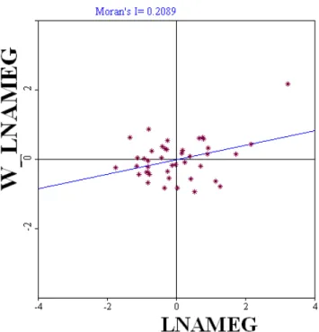
The value of I for the log of per capita GDP (LNAMEG) is 0.2089. The expected value for this statistic under the null hypothesis of no spatial correlation is E[I]=-0.0244. It appears that LNAMEG is spatially correlated since the statistic is significant with p=0.0140. This initial result therefore reveals the existence of a pattern of positive spatial dependence in the distribution of county wages in Romania. Map 2 shows the spatial distribution of county wages in Romania in 2006. Figure 3 provides a view that there is spatial autocorrelation in this year through the Moran scatterplot 9.
Map 1.2: Spatial percentile distribution for the log of Wages in 2006, (LnAMEG)
Source: Own elaboration based on INSEE data
9 The Moran scatterplot displays the spatial lag W log(GDPpc) against log(GDPpc), both standardized.
Figure 1.9: Moran scatterplot for the log of Wages in 2006
Source: Own elaboration based on INSEE data
1.6. Final Remarks and Conclusions
In this chapter we have built a New Economic Geography model an estimate an econometric specification which relates the levels of per capita GDP levels paid in each location with an index of the degree of accessibility to consumer markets in that location. The estimations have being performed for a sample of 42 Romanian regions for the year 2006. The chapter reports two main results: From our baseline estimations we have shown that market access play an important role in shaping the spatial wage structure observed in Romania. This first result has to be interpreted with caution insofar as the instruments for market access are weak. Turning to our preferred specification, our results also point to the fact that there are (at least) two important channels through which market access might be affecting the Romanian spatial wage structure which are human capital levels and regional innovation sizes. Therefore, these results emphasize the role of market access in avoiding Romanian wage differences to be bid away and so in acting as a penalty for the economic catching up of the poorest Romanian regions towards the more developed ones. This result has a clear implication in policy terms: as regions cannot change their location, i.e. regions cannot move, an obvious policy implication in this regard will be the need of implementing policy actions to reduce transport costs directly via improvements in infrastructure (e.g. roads, ports, etc.) which in the case of Romania are still very much lagging behind.
this respect the recent and converging debate on the interplay of human capital externalities theories and urban wage premium theories suggested in Halfdanarson et al. (2008) seems a worthwhile undertaking10. Very recently the collection of reliable micro-data on workers individual features in some countries has allowed performing very fine econometric studies to estimate the effect of individual skills in existing spatial wage disparities. Using French micro-data Combes et al. (2008) show that spatial sorting by skills is very important in explaining spatial wage disparities. In Spain, Puga and De la Roca (2010) have exploited a micro data base (based on Spanish social security records which traces over time the working places and the salaries for a very large sample of individuals) to analyze the dynamic effects in wages of working in dense cities. Once this kind of micro data becomes available for more countries (among them Romania) it would really interesting to enlarge the geographical focus of this type of studies and test for the robustness of the aforementioned studies. Finally, it will also be important to seek alternative channels that may be affecting per capita GDP levels in addition to human capital and innovation.
Chapter 2: Economic Geography, Human Capital and
Policy Implications in Romanian counties
11Abstract
This chapter looks at the link between human capital and geographical location for the Romanian regions based on the theoretical model developed in Redding and Schott´s (2003) chapter. Using 2006 data on the different educational attainment levels for the 42 Romanian regions, it identifies that the percentage of individuals with medium and high educational levels is affected positively by the regions´ market access. Doubling market access would increase the percentage of individuals with medium and high educational levels between 22-25%. We also disentangle the effects market access can have on higher educational attainment levels by looking for third variables that might be affecting regional educational levels and which work through accumulation incentives. Some policy implications to overcome the costs remoteness imposes on human capital accumulation in Romania are also drawn.
Key Words: Geographical location, Market Access, Human Capital, Romania
JEL Classification: R11, R12, R13, R14, F12, F23
11 A version of this chapter has been published as a working paper N.522/2010 of the Colección de
Documentos de Trabajo de la Fundación de las Cajas de Ahorros (FUNCAS) and as Lopez-Rodríguez, J., Faiña A. and C. Bolea-Gabriel (2011) The Effects of Economic Geography on Education in Romania,
counties
2.1. Introduction
Human capital can broadly be defined as “...the productive resources that focus on work resources, skills and knowledge" (OECD) or "human skills and capabilities generated by investments in education and health" (WHO). From these definitions it is clear that human capital must play an important role in the economic development of countries and regions. In fact, aggregate human capital at national or regional level has been a recurrent variable in economic growth models (Barro, 1991, 1997; Barro and Lee, 1994; Benhabib and Spiegel, 1994; Englander and Gurney, 1994; Hanushek and Kim, 1995; Islam, 1995). However, despite of the wide scholarly agreement of its impact on economic growth there is little consensus on the exact contributions of the different measures and indicators of human capital to economic development (Levine and Renelt, 1992; Rodriguez-Pose and Vilalta-Buffi, 2005). Another important issue related to human capital and economic development and far less studied is the role the economic geography of a country or a region plays with respect to this relationship. At this point the fairly new branch of the spatial economics known as New Economic Geography (NEG) (Krugman 1991, 1992) has emerged as a new theory which emphasizes the role second nature geography variables or economic geography variables play with respect to the spatial distribution of income and human capital across countries or regions as oppose to the role played by first nature geography 12 variables (Hall and Jones, 1999).
12 By first nature geography we refer to the physical geography of a country (natural endowments,
The emphasis of a large number of empirical studies in the NEG literature has been put on the effects economic geography have on either cross-country or cross-regional per capita income differences. This has been done by testing the well-known theoretical proposition that arises in standard core-periphery NEG models which is refer to as the nominal wage equation (Brakman et al., 2004; Breinlich, 2006; Hanson, 2005; Overman et. al., 2003; Redding and Venables, 2004; Lopez-Rodriguez and Faiña, 2007). However, recent theoretical developments within the NEG literature (Redding and Schott, 2003) has allowed to extend the empirical investigations to the analysis of the effects geographical location have on human capital accumulation.
counties
economic geography has on cross-country and cross-regional per capita income can be considered as an additional prove of the penalty remoteness imposes for economic development and therefore for the convergence of countries and regions. However, much more empirical studies on the relationship between human capital and location are needed. So far, there is only one paper at country level on the forces put at work in Redding and Schott´s (2003) paper.
This chapter tries to fill in this gap by applying Redding and Schott´s (2003) framework to the regions in a national setting such as the case of Romania. The chapter stresses, for the case of the 42 Romanian regions, the importance of geographical location in human capital accumulation, showing that the percentage of individuals with medium and high educational attainment levels depends positively on the region´s market access whereas the opposite occurs for low educational attainment levels.
The rest of the chapter is structured as follows: section 2 contains the theoretical framework in which the relationship between human capital accumulation and geographical location is established. Section 3 presents the econometric approach and data. Section 4 discusses the econometric results on the link between educational attainment levels and remoteness. Finally section 5 presents the main conclusions and some policy implications.
2.2. Theoretical framework
(2003) model is in the modelling of the role played by intermediate goods. Contrary to Redding and Schott´s (2003) model we assume that the production of manufactured goods is carried out without using intermediates in the production of final output. The difference of this model with respect to standard two-sector NEG models such as Fujita et al. (1999) or Krugman (1991) is based on the introduction of endogenous human capital accumulation. To account for this new feature we consider a world in which we have R locations
i
∈
{
1
,....,
R
}
and eachlocation have a mass of consumers Li. We assume that consumers are endowed with one unit of labour which is offered inelastically with zero disutility and that consumers choose endogenously whether to invest or not in becoming skilled. In the decision of becoming skilled a worker has to compare the costs of education to acquire those skills with the future benefits of been skilled, which for the purposes of this chapter can be summarized in the higher wages skilled workers perceive. Therefore, the critical part of the model is constructed over the individuals’ human capital investment choice, which is formulated as:
( )
w and wiurepresents the wage level of skilled and unskilled
workers respectively. The gap in the left-hand side of (2.1) is the wage premium, which should be higher than the cost of education defined in the right-hand side so that individuals have incentives to invest in education. The cost of education comprises two components:
( )
a z represents individuals’ ability to become skilled, which lowers the
counties
measure, i.e., increasing
h
i raises the cost of private education. From equation (2.1), Redding and Schott (2003) derived a skill indifference condition:a represents a critical level of ability at which individuals are
indifferent to becoming skilled or remaining unskilled. As the relative wages of skilled workers increase, the cut-off for this critical level of ability falls. In turn, this means that the number of individuals with an economic incentive for becoming skilled increases. Therefore, it is the magnitude of the relative wage that determines the individuals’ decision to invest in human capital.
In the same way as in standard models of NEG, this model assumes homothetic utility functions and the same preferences for all consumers, which are defined for the consumption of a homogeneous agricultural good and a set of differentiated manufactured goods. Focusing on the agriculture and manufacturing equilibrium conditions of the model, it is easily to endogenized human capital accumulation as a function of the geographical location of the regions.
i
Y
represents the output of the agricultural sector. In this sector theoutput is produced using a φ share of skilled workers and a 1−
φ
shareof unskilled workers.
θ
i is a parameter representing the agricultural productivity in each location.The manufacturing sector produces differentiated goods according to a technology which presents increasing returns to scale and where the production of each variety requires only primary factors of production (skilled and unskilled labour). The profit function of a typical firm at location ican be given by the following expression:
∑
c
is a marginal input specific to each location representing a technologyindex. F is a fixed cost of production and
∑
produced by the company for all markets it serves. Manufactured goods are traded between different locations incurring iceberg transportations costs, in other words a fraction of the good carried from location i to
location