Beyond earned value management: a graphical framework for integrated cost, schedule and risk monitoring

(1)

Procedia - Social and Behavioral Sciences 74 ( 2013 ) 181 – 189

26

th

IPMA World Congress, Crete, Greece, 2012

Beyond Earned Value Management: A Graphical Framework

for Integrated Cost, Schedule and Risk Monitoring

Fernando Acebes

a

, Javier Pajares

a,*

, José Manuel Galán

b

, Adolfo López-Paredes

a

a_{INSISOC, University of Valladolid, Valladolid, Spain} b_{INSISOC, University of Burgos, Spain}

Abstract

In this paper, we propose an innovative and simple graphical framework for project control and monitoring, to integrate the dimensions of project cost and schedule with risk management, therefore extending the Earned Value methodology (EVM). EVM allows Project managers to know whether the project has overruns (over-costs and/or delays), but project managers do not know when deviations from planned values are so important that corrective actions should be taken or, in case of good performance, sources of improvement can be detected. From the concept of project planned variability, we build a graphical methodology to know when a project remains “out of control” or “within expected variability” during the project lifecycle. To this aim, we define and represent new control indexes and new cumulative buffers. Five areas in the chart represent five different possible project states. To implement this framework, project managers only need the data provided by EVM traditional analysis and Monte-Carlo simulation. We also explore the sensitivity of the methodology to control variables.

Keywords: Earned Value Management; risk management; project control and monitoring

1.Introduction

Earned Value Management (EVM) is one of the most widely used and known methodologies for project control and monitoring. EVM integrates scope, cost, time and schedule under the same framework. Developed by the U.S. Department of Defense during the sixties, it allows project managers to measure and verify the progress of the project and to detect deviations from the project planning phase,

*_{Corresponding author: Tel.: +34 983 185954.}

E-mail address: [email protected].

Selection and/or peer-review under responsibility of IPMA

Open access under CC BY-NC-ND license.

(2)

so that early corrective actions could be taken. New cost and time forecasts can also be computed taking into account deviations under different hypotheses.

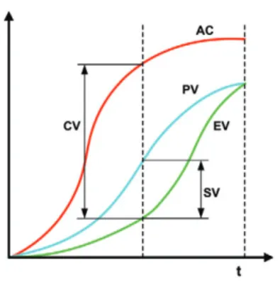
A detailed explanation of the methodology and its implementation can be found in Anbari (2003), Fleming & Koppelman (2005) and PMI (2005). EVM is based on three basic variables: Planned Value (PV) or budgeted cost of work scheduled; Actual Cost (AC) or the actual cost of work performed; and Earned Value (EV) or the budgeted cost of the work performed. From the basic variables, four indexes are defined: Cost Variance (CV = EV-AC), Schedule Variance (SV = EV-PV), Cost Performance Index (CPI = EV / AC) and Schedule Performance Index (SPI = EV /PV). Whenever CV<0 and CPI<1 there are over costs, and whenever SV<0 and SPI<1, the project is delayed. Positive values of SV and CV mean the project is in advance from plan and under budget respectively. Variables and variances can be represented graphically (see Figure 1), helping project managers to monitor project evolution. The graphical representation of PV is the project cost baseline.

Lipke (2003, 2004) proposed an extension of the methodology: the concept of Earned Schedule (ES). ES solves some problems faced by the methodology regarding its forecasting capabilities during the last phases of the project lifecycle. ES is the date when the current earned value should have been achieved. Schedule variance and performance indexes can be re-defined in terms of ES (SV(t)=ES-AT and SPI(t)=ES/AT, where AT is actual time).

Fig. 1. EVM main variables and variances

The integration of risk analysis under the EVM framework represents an interesting step forward in the development of the methodology. EVM variables and variances talk about what happened in the past, whereas risk management is concerned about the future. Pajares & Lopez-Paredes (2011) proposed to integrate both perspectives under the same framework, so that project managers could enjoy new tools for taking better decisions.

Vanhoucke (2011) proposed to monitor the projects under two perspectives: a top-down approach based on earned value metrics and a bottom-up approach based on the schedule risk analysis method. He shows that the efficiency of the each approach depends on the features of the project network. Vanhoucke (2012) used Monte-Carlo simulations to explore why EVM and Schedule Risk Analysis provide good results in some projects and poor results in others. Hazir & Shtub (2011) used EVM measures to monitor projects and develop a simulation software to replicate uncertain environments. They explore the relation between information presentation and project control.

(3)

Project variability can be estimated during the planning phase by means from Monte-Carlo simulations from the activity probability distributions; therefore, there is a “planned or expected variability” of the project at any moment during the project run. As a consequence, project overruns could be, at any time, inside or outside this variability.

EVM variances and indexes show whether the project is delayed or presents over-costs, but they do not say whether these overruns are within the planned variability or not. If they are not, corrective actions should be taken, as some structural changes or external unexpected events could have taken part in the project runtime. To this aim, Pajares & Lopez-Paredes (op.cit.) propose two new indexes: the Schedule Control Index (SCol) and the Cost Control Index (CCol).

In this paper, we give a step forward and we propose a graphical framework, easy to build, to help project managers to know when project performance is out of the planned variability and corrective actions should be taken to assure the project finishes under the planned schedule and budget. The methodology does not need more information than the calculations performed in EMV analysis and the Monte-Carlo simulation methodology.

The rest of the paper is structured as follows. In section 2 we briefly review the calculations of the Schedule and Cost Control Indexes; in section 3, we describe the graphical framework we propose in this paper, and the different scenarios that can be analyzed with it. In section 4 we show the influence of some control parameters in the methodology. We finish with the main conclusions of our work.

2.The Schedule and Cost Control Indexes

Most of the scheduling methodologies include uncertainty, as they suppose that activity durations follow a statistical distribution function. The same reasoning can be applied to activity cost variability. Monte-Carlo analysis allows project schedulers and accountants to know about the statistical distribution of the final project duration and total cost. This way, we can compute, for instance, the maximum cost at a confidence level pc, that is the value (Pc) that satisfies that the probability of the project cost to be lower

than Pc is pc. The same applies to schedule distributions (Ps, ps). However, project managers do not want

to wait until the end of the project to see whether the project has finished “statistically on time”; they need measures during project runtime in order to take the appropriate decisions.

Pajares & Lopez-Paredes (op.cit.) define the Project Risk Baseline as “the evolution of ‘project risk value’ through project execution lifecycle. The risk of the project at any given time is calculated as the risk of the project pending tasks (those not yet completed), assuming that the project has performed as planned until that given time”. A Risk Baseline can be defined for schedule (SRB) and other one can be defined for cost (CRB). The evolutions of risk baselines indicate how risk is “eliminated” during project runtime; therefore, the risk reduction at time t can be computed as:

wct = CRBt 1 CRBt wst = SRBt 1 SRBt (1)

The project total buffers (cost and schedule) are computed as:

CPBf = |Cmean – Pc| SPBf = |Smean – Ps| (2) where Cmean and Smean are the mean project cost and mean project duration computed by means of

Monte-Carlo simulations. This buffer applies at the end of the project, and it means that, with a confidence of pc (ps), the project cost (schedule) will remain less than Pc (Ps), whenever the project

(4)

CBft = wct*CPBf / 2_{Pc SBft = wst*SPBf /} 2_{Ps (3)} where 2

Pc and 2Ps are the total cost and schedule statistical variance, computed by means of Monte-Carlo simulation. Now it is possible to compute the cumulative buffers at time t.

ACBft = CBft + ACBft 1 ASBft = SBft + ASBft 1 (4) and finally, if we compare these cumulative buffers with the variances from EVM, we obtain the

control indexes:

CCoIt = ACBf(t=ES)+ CVt = ACBf(t=ES)+EV AC (5)

SCoIt = ASBft + SV(t) = ASBft + ES AT (6)

where CCoIt and SCoIt are the Cost Control Index and the Schedule Control Index respectively. If CColt (SColt) is negative, over costs (delays) will exceed the cumulative “natural” variability of the project, as project variances (cost or schedule) will be higher (in absolute value) than the cumulative buffer.

3.The graphical framework for project control

In order to build up the graphical control framework, we draw the following curves: The control indexes: SCol and CCol, from equations (5) and (6)

The cumulative buffers: ASBf and ACBf, from (4). In particular, we will split equations (2) and will consider a minimum and a maximum cumulative buffer:

CPBfmin = Cmean – Pc,min ; SPBfmin = Smean – Ps,min CPBfmax = Pc,max – Cmean ; SPBfmax = Smean – Ps,max

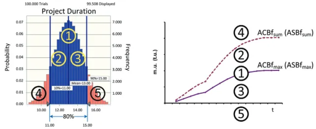
Pmin and Pmax must be decided by the the project manager, as this election determine the amplitude of the control limits. Usually, the common lover and upper limits are related to the probabilities of 10% and 90% respectively (see Figure 2); we will use these values in this paper. Then, we will use equations (3) and (4) to compute the cumulative buffers ACBfmax,t (ASBfmax,t) and ACBfmin,t (ASBfmin,t). Finally, we will represent the curves

ACBfmax,t and ACBfsum,t = ACBfmin,t+ ACBfmax,t ASBfmax,t and ASBfsum,t = ASBfmin,t+ ASBfmax,t

where ACBfsumand ASBfsum are computed by simple addition of the maximum and minimum buffers. Whenever the statistical distribution of the cost (schedule) is symmetric, and mean equals mode, then both buffers become equal and ACBfsum=2*ACBfmax (ASBfsum=2*ASBfmax).

ASBf’s and ACBf’s are computed using the data from the planning phase calculations, as we only need the risk baselines and the project schedule and cost statistical variances, all of them computed by means of Monte-Carlo simulations (see Figure 2a). The control indexes (SCol and CCol) are computed during project runtime from the EVM calculations.

Within this approach, we distinguish among five different scenarios due to the relative values of the control indexes SCoI and CCoI in relation to the cumulative buffers (Figure 2b).

(5)

Fig. 2. a) Project duration probability function. b) Graphical framework.

3.1.The cumulative maximum buffer line

When the project is running according to schedule, SV(t)=0 and, as a consequence, SColt=ASBft This means that the project control index lies within the line 1 in Figure 2. In any case, even if the project had overruns in the past, but then it moved again to planning conditions, the control index will be again within the cumulative buffer line.

If the project is delayed, SV(t)<0, and then SColt<ASBft , no matter how negative SV(t) is. Therefore, whenever the project is delayed, the control index remains below the cumulative buffer line 1 (areas 3 and 5 in Figure 2). On the other side, if the project is behind schedule, SV(t)>0 and SColt>ASBft , and the

control index remains above the cumulative buffer line (areas 2 and 4 in Figure 2).

This means that the cumulative buffer line plays the same role than the x-axis in the schedule variance graph used in EVM analysis. In other words, it gives us the same information. But under the new framework, we can not only know whether the project is delayed or ahead of schedule, but also can see whether this delay is within the planned project variability or not.

3.2.The x-axis line

Whenever the project is delayed, then SV(t)<0. But there are two possibilities:

|SV(t)|>ASBft . Then, SColt<0 and this mean that the delay is higher than the acceptable delay within the planned variability. The project management team should study whether some unexpected events have taken place in the project, and, if necessary, they should take early corrective actions. This happens in area 5 in Figure 2.

|SV(t)|<ASBft . This means that SColt>0 and the project remains under the planned conditions. Area 3 in Figure 2.

(6)

3.3.The sum of cumulative minimum and maximum buffer lines

Whenever the project is ahead of schedule, SV(t)>0, and as we showed in subsection 3.1., SColt>ASBft. But again, the amount of advancement can be or not within the range of probable results derived from the planned project variability. To know the situation the project is in, we must compute the cumulative minimum buffer line ASBfmin,t:

If the project remains within the planned conditions, then SV(t)<ASBffmin,t , therefore: SColt=ASBfmax,t+SV(t)<ASBfmax,t+ASBfmin,t= ASBfsum,t

and the control index figure remains within area 2 (Figure 2).

Finally, if the project is more advanced than it should be according to planning variability, SV(t)>ASBffmin,t , and as a consequence, SColt=ASBfmax,t+SV(t)>ASBfmax,t+ASBfmin,t

Therefore, the curve ASBfsum,t = ASBfmax,t+ASBfmin,t, allows project managers to know whether the project is running within planned conditions or not (areas 2 and 4 respectively in Figure 2). Although the project is ahead of schedule in both cases, project management team should play close attention to situations where the advancement is higher than expected, as it means that some unplanned events are taking place in the project, and they could be a source of opportunities for further improvements.

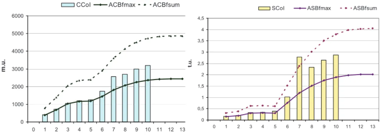
In Figure 3, we show a practical example. Control indexes are represented by means of bars, whereas the two lines show de evolution of ACBfmax,t and ACBfsum,t (ASBfmax,t and ASBfsum,t). The cumulative buffers are computed by means of the data from Monte-Carlo simulations, and the control indexes are computed during project runtime.

In Figure 3, actual time is 10 periods and the project is under budget and ahead of schedule, but these improvements remain under the planned variability.

4.Sensitivity to control limits

The values of pmin and pmax determine how wide or narrow the control is. In practice, levels of 10% and

90% are commonly used, as they cover the 80 % of the area of the project total duration (cost) statistical function. In this section we study the influence of the control limits, as they will affect both the control indexes and the cumulative buffers.

0

(7)

For a particular project, in Figures 4 and 5 we show two different control environments: the wider one is drawn in Figure 4, where pmin and pmax are 10% and 90 %, with values of Pmin=11 t.u. (time units) and

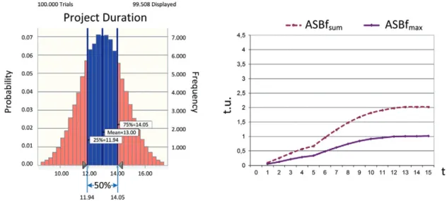
Pmax=15 t.u. The narrower environment is shown in Figure 5, with probabilities of 25 % and 75 % and

values of 11.95 and 14.06. In both cases, the dark surface under the project duration probability function in Figures 4a and 5a expresses the probability of the project to finish between the control limits.

Fig. 4. Control limits: 10%, 90%. a) probability function, b) cumulative buffers.

Fig. 5. Control limits: 25%, 75%. a) probability function, b) cumulative buffers.

(8)

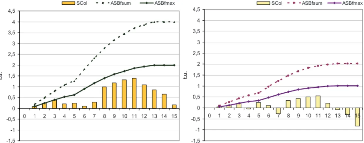
control index equals the cumulative maximum buffer (SCol=ASBfmax).Then, the project is delayed as the Schedule Control Index is bellow the cumulative buffer line. But in the (10%, 90%) case (Figure 6a) the control index is always positive, that is, the project duration always remains within the control limits and the project manager will not be warned about unexpected events. In the narrower case (25%, 75%), the Schedule Control Index became negative at period 7 and after period 13 (Figure 6b), alerting project manager about not planned changes.

-1,5

Fig. 6. a) 10,90 scenario, b) 25,75 scenario.

When the control is narrow, warning signals are more frequent, therefore a trade-off must be reached in order to manage the project properly.

5.Conclusions

We have proposed a simple graphical framework for project control. We represent the evolution of the control indexes proposed by Pajares & Lopez-Paredes (op.cit.) and we add two new measures: the cumulative maximum buffer and the sum of the cumulative minimum buffer and the cumulative maximum buffer. With these new measures, the project manager can determine graphically whether the project is delayed or not and whether the departure from planned values remains within the expected or planned variability (similar reasoning applies to cost). If overruns are higher than the allowed values, corrective actions should be taken in order to drive the project to control. If good performance is achieved, the methodology alerts project managers about possibilities of improvement.

The framework includes all the information deductible from EVM analysis, but in addition integrates risk analysis and the concept of project planned variability.

(9)

Acknowledgements

This research has been financed by the project “Computational Models for Strategic Project Portfolio Management”, supported by the Regional Government of Castile and Leon (Spain) with grant VA056A12-2.

References

Anbari, F. T., (2003). Earned Value Project Management method and extensions. Project Management Journal; 34(4), pp. 12-23.

Fleming, Q., & Koppelman, J. (2005). Earned Value Project Management. Third ed. Project Management Institute, PA: Newtowns Square.

Hazır, Ö., & Shtub, A., (2011). Effects of the information presentation format on project control. Journal of the Operational Research Society, 62, pp. 2157-2161.

Lipke, W. (2003). Schedule is different. The Measurable News (Summer), pp. 31-34.

Lipke, W., 2004. Connecting earned value to the schedule. The Measurable News, Winter 1, pp. 6-16.

Pajares, J. & Lopez-Paredes, A. (2011). An extension of the EVM analysis for project monitoring: The Cost Control Index and the Schedule Control Index. International Journal of Project Management, 29(5), pp. 615-621.

Project Management Institute (PMI), 2005. Practice Standard for Earned Value Management. Project Management Institute, Newtown Square, PA.

Vanhoucke, M., (2011). On the dynamic use of project performance and schedule risk information during project tracking. Omega, 39, pp. 416-426