Implementation of User Element Subroutines for Frequency
Domain Analysis of Wave Scattering Problems with
Commercial Finite Element Codes
Felipe Mosquera-Arias
[email protected]
Grupo de Mec´
anica Aplicada
Departamento de Ingenier´ıa Civil
Escuela de Ingenier´ıa
Universidad EAFIT
Implementation of User Element Subroutines for Frequency Domain
Analysis of Wave Scattering Problems with Commercial Finite Element
Codes
Felipe Mosquera-Arias
[email protected]
A thesis submitted to the
Faculty of the Civil Engineering Department
Universidad EAFIT
in partial fulfillment of the requirements for the
degree of
Master of Science
Nota de aceptaci´on
Presidente del jurado
Jurado
Jurado
Acknowledgements
Table of Contents
Abstract 1
Introduction 2
1 The Wave Scattering Problem in Elastodynamics 7
1.1 Boundary Value Problem Governing the Scattering of Elastic Waves . . . 8
1.1.1 Differential Formulation . . . 8
1.1.2 Integral Formulation of the Boundary Value Problem . . . 11
2 User Element Subroutine 15 2.1 Discrete Formulation of a Generalized Wave Scattering Problem . . . 16
2.2 Finite element formulation in real algebra . . . 18
2.3 Scattering of plane waves . . . 22
2.4 Verification Problems . . . 25
2.4.1 Simple Elasticity Problem . . . 25
2.4.2 Scattering of Plane P waves by a Cylindrical Canyon in a Half-Space . . . . 27
3 The Problem of Site Effects in Earthquake Engineering 29
TABLE OF CONTENTS iv
3.1 The role of diffraction in the site effects problem . . . 30
3.1.1 Prediction of the diffracted field . . . 32
3.1.2 Scattering of P and SV waves by a semicircular and a rectangular canyon . 36
3.2 The modified domain reduction method: Application to topographic effects . . . 45
3.2.1 The domain reduction method . . . 45
3.2.2 Application to topographic effects. . . 47
4 Scattering in a Micropolar Solid 54
4.1 Non-classical Cosserat micropolar material . . . 56
4.2 Finite Element formulation. . . 57
4.3 Scattering of P waves by a semicircular canyon in a micropolar half-space . . . 60
Conclusions and Further Work 65
A Sample Problem: Scattering by a Semicircular Canyon 68
List of figures
1.1 Schematic description of the scattering problem. . . 9
1.2 Definition of the domain and the different instances appearing in the BEM schemes 14 2.1 Definition of the degrees of freedom in a FEM discretization. . . 17
2.2 Definition of the problem domain. . . 23
2.3 Assemblage for static validation of the implemented user element subroutine. . . 25
2.4 Nodal displacements corresponding to the manual solution. . . 26
2.5 Nodal displacements corresponding to the UEL solution. . . 27
2.6 Finite element mesh for the semi-circular canyon. . . 28
2.7 Spatial distribution for the frequency domain transfer function over the canyon surface for a dimensionless frequency η = 1.0. The function corresponds to the amplitude of the Fourier spectral response normalized over the amplitude of the incident wave. The function on the left corresponds to vertical incident and the one in the right to 30.00 incidence. . . 28
3.1 Definition of the problem domain. . . 33
3.2 Classical partition of the total solution into free field plus scattered motions. . . 34
3.3 Partition of the solution into incident, physically reflected and diffracted fields. . . . 34
3.4 Geometrical theory solution for the semicircular canyon. . . 35
LIST OF FIGURES vi
3.5 Response of the rectangular and semi-circular canyons to SV waves incident at
θ = 00 and θ = 300. The results shown in rows 1 and 2 correspond to the spatial distribution over the free surface of the frequency domain transfer function at the characteristic frequencyfc = 1.0Hz associated with the diffracted (row 1) and total
(row 2) vertical displacement component. The results in row 3 are the synthetic seismograms over the canyon surface in each case. The first two columns correspond to the rectangular canyon and columns 3 and 4 to the circular canyon. . . 39
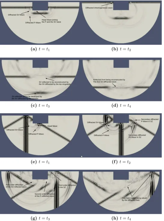
3.6 Response of the rectangular canyon to a vertically and a 300 incident SV wave. The snapshots correspond to full particle motions. The full videos are available at
http://www.youtube.com/watch?v=gen5mNxJPiwandhttp://www.youtube.com/ watch?v=NdijUjEWfAI&feature=youtu.be . . . 40
3.7 Response of the semi-circular canyon to a vertically and a 300 incident SV wave. The snapshots correspond to full particle motions. The full videos are available at
http://www.youtube.com/watch?v=tlCKdgmioGY&feature=youtu.be and http: //www.youtube.com/watch?v=qcq-WYMEvSY&feature=youtu.be . . . 41
3.8 Synthetic seismograms for the semi-circular and rectangular canyon under incident
SV and P waves. Row 1 correspond to the SV case in the rectangular canyon. Row 2 correspond to theSV case semi-circular canyon. Row 3 correspond to theP
case in the rectangular canyon. Row 4 correspond to theP case in the semi-circular canyon. Columns 1 and 2 depict the horizontal and vertical field for 0.00 incidence while columns 3 and 4 depict the horizontal and vertical fields for 30.00 incidence. . 42
3.9 Transfer functions for the semi-circular and rectangular canyon under incident SV
and P waves. Row 1 correspond to the SV case in the rectangular canyon. Row 2 correspond to the SV case semi-circular canyon. Row 3 correspond to the P case in the rectangular canyon. Row 4 correspond to the P case in the semi-circular canyon. Columns 1 and 2 depict the horizontal and vertical field for 0.00 incidence while columns 3 and 4 depict the horizontal and vertical fields for 30.00 incidence. . 44
3.10 Full domain considering a structure and a micro-zone. . . 45
3.11 Reduced domain with the micro-zone and structure being removed. . . 46
3.12 Final domain for the micro-zone excited with the response from the reduced domain. 46
3.13 Simplified model equivalent to the Aburr´a valley with a localized soil deposit.. . . . 47
3.14 Set of points near a microzone where the regional solution is stored. . . 48
LIST OF FIGURES vii
3.16 Spatial distribution of the frequency domain transfer functions for the horizontal and vertical component of the response at three different values of the non-dimensionless frequencyη for receivers located over the microzone surface. . . 49
3.17 Fourier spectral amplitude at the central point of the microzone obtained with the complete model, DRM-model and classical model. . . 50
3.18 Synthetic seismograms at the central point of the microzone obtained with the complete model, DRM-model and classical model. . . 50
3.19 Simplified model equivalent to the Aburr´a valley with a localized soil deposit.. . . . 51
3.20 Spatial distribution of the frequency domain transfer functions for the horizontal and vertical component of the response at three different values of the non-dimensionless frequencyη for receivers located over the inclined microzone surface. . . 52
3.21 Fourier spectral amplitude at the central point of the microzone obtained with the complete model, DRM-model and classical model for the second microzone. . . 52
3.22 Synthetic seismograms at the central point of the microzone obtained with the complete model, DRM-model and classical model for the second microzone. . . 53
4.1 Dispersion for the micropolar waves. . . 55
4.2 Spatial distribution of the transfer function along the cavity surface under vertically incident P waves. . . 61
4.3 Synthetic seismograms for the semi-circular canyon in a micropolar half-space under vertically incidentP waves. . . 62
4.4 Frequency domain transfer functions for the classical canyon (left) and micro-polar canyon (right) for receivers over the canyon surface. . . 63
4.5 Synthetic seismograms for the horizontal and vertical fields over the semi-circular canyon surface with the classical material (left) and the micro-polar material (right). 63
4.6 Snapshots of the propagation patterns in the semi-circular canyon with a classical model (left) and a micro-polar model (right). The full video is available at http: //www.youtube.com/watch?v=y-3j5BdTDaw&feature=youtu.be . . . 64
LIST OF FIGURES viii
Abstract
A user element subroutine (UEL) to be used into the commercial finite element code ABAQUS has been developed and implemented. The subroutine is intended to treat generalized wave propagation problems in 2D-domains and in particular wave scattering problems. It has been formulated in the frequency domain, but fully implemented in terms of real-valued degrees of freedom as required by ABAQUS. Results are obtained both in the frequency and time domain. The subroutine is tested in the solution of problems related to topographic effects in earthquake engineering and in the propagation of waves in materials with microstructure introducing dispersion. Results have been provided in the frequency and in the time domain. The frequency domain is not only powerful from a conceptual point of view, since it offers many insights into the physical aspects of the problem, but it also has other advantages like:
• Easy incorporation of excitations based on plane wave assumptions.
• Simultaneous Consideration of temporal and spatial periodicity.
• Easy consideration of dispersive materials.
Keywords: Wave Propagation, Computational Elastodynamics, Finite Element Methods,
Boundary Element Methods, Seismic Waves, Periodic Materials.
Introduction
The phenomenon of wave propagation appears in many different engineering fields, e.g., electro-magnetism, acoustics, mechanics. At the same time, computational methods have evolved to the point, where simulation based engineering is increasingly being used by the practising engineer in order to support lab results, improve proposed designs or even to compensate for the lack of experimental data. In the case of mechanical waves, the subject is of interest in diverse engineering topics like, earthquake engineering; geophysics; mechanical characterization of materials; and oil and natural gas exploration, among others.
Although computational mechanics based techniques, allow the problem of wave propagation to be solved with great accuracy, the existing commercial tools still pose limitations to the user, due to different factors. For instance, commercial codes are limited in the type of available kinematic assumptions, they only have a few constitutive material models and they are also limited in the possible forms of excitation. These limitations have kept a lot of problems of wave propagation within the strict realm of academics and researchers. One of the major limitations in commercial codes is the impossibility of performing analysis in the frequency domain with enough flexibility in the type of excitation, mainly because most commercial software don’t allow the user to pass complex-valued information. This limitation is taken care of in this thesis.
In this work a computational tool for the simulation of generalized wave propagation problems in the commercial finite element code ABAQUS is presented. The computational framework is developed in the form of a user element subroutine (UEL), which is a possibility offered to the user by commercial codes, like ABAQUS, to overcome limitations in the type of analysis implicit in the code. This work has been motivated by a need identified within the Grupo de Mec´anica Aplicada at Universidad EAFIT to solve wave propagation problems of moderate size (e.g., in the range of millions of degrees of freedom), when working in the particular context of earthquake engineering.
The subroutine takes advantage of the powerful simulation resources available in the commercial code, like its pre and post-processing units and efficient solvers, allowing the analyst to simulate a complex problem, not available in the code, but with the easiness of data input implicit in a robust commercial software.
Although the current UEL subroutine is developed in the context of earthquake engineering, it
3
is general enough and straight forward to modify as required, so it can be easily extended to many different applications and physical areas. This generality is possible, since the analysis is conducted in the frequency domain but in terms of real algebra calculations. In this sense ABAQUS is used as a solver for a series of generalized static problems while being unaware of the type of physical problem being solved. The particular implementation uses the idea of generalized variables to proceed in the frequency domain, but expressing the problem in terms of real valued functions. The frequency domain is not only powerful from a conceptual point of view since it offers many insights into the physical aspects of the problem, but it also has other advantages like:
• Easy incorporation of excitations based on plane wave assumptions.
• Simultaneous consideration of temporal and spatial periodicity.
• Easy consideration of dispersive materials.
Although the main objective of this thesis is the formulation and implementation of the UEL subroutine into the commercial FEM code ABAQUS, several problems have been solved in order to test and show the subroutine’s current capability. The following problems have been solved:
• Scattering of incident in-plane P waves by surface shapes in a micropolar solid. The scat-tering of waves by a geometric irregularity embedded in a non-classical material model has been studied in order to simulate a dispersive medium. For this purpose a Cosserat or kinematically enriched material model has been numerically simulated.
• Scattering of incident in-planeP andSV elastic waves by surface scatterers. The context of the analysis corresponds to the problem of topographic effects in earthquake engineering. A method, based on the isolation of the diffracted part of the response has been presented and explored, where the diffraction field is used as a digital finger print of the topographic effect.
• Study of the topographic effects in a simplified model of a sedimentary basin with a cross section resembling the Valle de Aburr´a. A domain reduction method has been explored as a potential analysis tool to establish the connection between large geometrical or regional topographic effects and localized mechanical effects like the ones existing in seismic micro-zones.
The routine capabilities include:
4
• Point source wave propagation analysis in infinite and semi-infinite domains using absorbing boundaries.
• Simulation of homogeneous and heterogeneous domains.
• Flexibility of boundary conditions like topographies of arbitrary shapes or dams in a strong topographic environment.
• Results in the frequency domain in the form of spatial transfer functions between response and incident motions and in the form of Fourier spectral amplitudes at a given point.
• Results in the time domain in the form of synthetic seismograms at user defined receivers and videos of the propagation patterns inside the complete computational domain.
• Easy consideration of dispersive materials.
The implemented UEL subroutine has been tested in a standard desktop computer with 16Gb of memory. Models as large as 6’000.000 degrees of freedom have been solved. The UEL subroutine and the post-processing software can be downloaded freely from the Mec´anica Aplicada web site
http://mecanica.eafit.edu.co/mecanica/.
This report is organized as follows. In the first chapter the wave scattering problem in elastody-namics is reviewed in differential and integral form. The formulation used by Bielak & Christiano (1984) in terms of total motions inside the scatterer and scattered motions inside the half-space is presented. Chapter 2 describes aspects of the algorithm used in the solution of wave scattering problems within the context of the finite element method (FEM). The idea of generalized variables and a generalized principle of virtual displacements in complex algebra as required by the frequency domain is introduced. The principle is then discretized but treating the real and imaginary parts independently. In this chapter a couple of simple verification problems are solved. Applications of the subroutine start in Chapter 3 with the problem of topographic and site effects in earthquake engineering and continue in Chapter 4 with the diffraction and scattering of waves in a micro-polar half-space. Conclusions and recommendations for further work are presented in the final part.
In the next section we include a brief review of the historical development of numerical methods mainly in earthquake engineering.
Literature Review
5
mechanical testing techniques among many others.Solutions can be obtained via numerical simu-lation and where complex combinations of geometry, material properties and boundary conditions can be considered. An extensive amount of work on the subject from the numerical point of view has been conducted during the last 30 years. Moreover, it has has been approached with different techniques depending on the specific type of problem and available computer requirements.
In the case of infinite or semi-infinite media problems-as is the usual scenario in earthquake engineering and geophysics-one of the challenges in the numerical solution, is the proper impo-sition of radiation boundary conditions. This problem can be dealt with in a very natural way, using integral equations formulations and its discretization in terms of different versions of the boundary element method. In that approach the radiation condition is implicit in the specific problem Green’s function. Solutions through different versions of the direct and indirect boundary element method and corresponding to problems in different physical contexts are reported inWong & Jennings (1975), citesills1978scattering, S´anchez-Sesma & Rosenblueth (1979), S´anchez-Sesma (1983), Dravinski & Mossessian (1987), Zhang & Achenbach (1988), Kawase (1988), Manolis & Beskos(1988), Kawase & Aki(1989), Mossessian & Dravinski (1989),S´anchez-Sesma & Campillo (1991), Kim & Papageorgiou (1993), Papageorgiou & Pei (1998), Janod & Coutant (2000), Itur-rar´an-Viveros et al. (2005), Sohrabi-Bidar et al. (2010). Although BE-based solutions are very accurate, its effective application to real size problems is very limited due to large computing requirements. As a result, the method is currently being used as a tool to perform parametric analysis in conceptual problems.
The first numerical solutions of wave diffraction problems with full domain methods, combined with absorbing surfaces to represent the radiation condition were obtained in terms of classical finite difference algorithms e.g.,(Boore, 1972; Archuleta & Frazier, 1978;Archuleta & Day, 1980). One of the major drawbacks of finite difference schemes, is the appearance of numerical dispersion near zones of large gradients of the field. Moreover, in large scale simulations–representative of realistic problems–the balancing of the trade-off between numerical dispersion and computational cost, turns out to be rather difficult, Komatitsch & Vilotte (1998). This numerical phenomenon can be avoided using staggered-grid formulations (e.g., (Madariaga,1977;Virieux,1986;Levander, 1988; Moczo et al., 2007). Additional works using finite difference schemes, although mainly related to seismic engineering problems, can be identified in Vidale & Helmberger (1988) in the study of surface waves with a 2D model of the Los Angeles basin, Frankel & Vidale (1992) in the response of the Santa Clara Valley to the 1989 Loma Prieta earthquake using one of the first full 3D models, Frankel (1993) in the response of the San Bernardino valley, Graves (1996) with a model of the Marina district in California using staggered grids and similar works likeYomogida & Etgen(1993),Olsen & Archuleta(1996),Stekl & Pratt(1998). Finite difference schemes combined with other techniques to effectively account for free surfaces and general boundary conditions still dominate the spectrum of numerical treatments of wave propagation problems.
6
element method. Early solutions to wave propagation problems were reported byLysmer & Drake (1972), Smith (1975), Ohtsuki & Harumi (1983), Mita & Luco (1987), Toshinawa & Ohmachi (1992). The first large scale simulation with FEM implementations were performed by Bao et al. (1998), who proposed and explicit algorithm embedded into an octree-based data storage scheme allowing for the simulation of real large scale problems; the resulting algorithm however, was restrained to problems without the consideration of topographic effects. These set of algorithms were later improved byBielak et al.(2003) andYoshimura et al.(2003), where a domain reduction method that allowed to effectively translate the source effects near the scatterer was proposed and by Bielak et al. (2009),Taborda & Bielak (2010), where problems of frequencies up to 5.0Hz and billions of elements have been solved.
Chapter 1
The Wave Scattering Problem in
Elastodynamics
Introduction
The problem of scattering and diffraction of elastic waves, by mechanical and geometrical irregu-larities, located over infinite or semi-infinite domains, is relevant in the analysis and design of civil engineering structures subject to seismic events. In particular, there is a strong interest in finding the appropriate design motions, when an incident seismic field interacts with a discontinuity in the form of surface or subsurface topography. In the context of earthquake engineering the prob-lem is termed the site effects probprob-lem, while in the more general context of the theory of wave propagation, it is referred to like a scattering problem.
Mathematically, the problem corresponds to an Initial Boundary Value Problem (IVBP) satis-fied over a semi-infinite domain and it is defined as follows: If one considers a prescribed incident field, impinging over a geometrically perturbed half-space (that is, a half-space with a disconti-nuity), the incident motions are modified by the geometrical disturbances, which subsequently become sources of scattered motions. The purpose of the analysis is the determination of the total displacements inside the scatterer and of the scattered motions over the half-space.
In the first part of this chapter, the differential equations representing mechanical equilibrium and the corresponding boundary conditions for the scatterer and the supporting half-space are formulated. The resulting boundary value problems in each domain, are then welded together through displacement and tractions compatibility arguments along their common coupling surface S. This yields a single well-posed BVP for the complete scatterer-half-space system. Considering the full problem, it becomes evident that the half-space plays the roll of a radiation boundary condition for the scatterer, carrying with it the sources and proper support conditions to be
CHAPTER 1. THE WAVE SCATTERING PROBLEM IN ELASTODYNAMICS 8
prescribed along the common coupling interfaceS. This work deals precisely with the imposition of radiation boundary conditions in terms of Half-Space Super Elements (HSSE), that can be incorporated into the scatterer discrete equilibrium equations in a commercial finite element code.
In the second part of the chapter, we formulate the BVP in the alternative form of integral equations, with the aid of the elastodynamics representation theorem. The discrete versions of this alternative formulations give rise to boundary element numerical schemes. As a result, the following discrete approximations would be possible within the context of this work;
• An approximation in terms of a domain of standard finite elements combined with silent boundaries.
• A semi-analytic description in terms of a boundary integral equation for the half-space using the specific half-space Green’s function.
• An approximation in terms of a boundary integral equation for the half-space using a full-space Green’s function and prescribed incoming motions.
In this work we only implemented the first of the above three approaches but extension to the other two is straight forward.
1.1
Boundary Value Problem Governing the Scattering of
Elastic Waves
1.1.1
Differential Formulation
CHAPTER 1. THE WAVE SCATTERING PROBLEM IN ELASTODYNAMICS 9
~
u(~x, t) =
+∞ Z −∞ +∞ Z −∞ ˆ ˆ ~
U(ˆi~κ,ˆiω)e−ˆi~k·~xd~κeˆiωtdω.
The reduced wave equation is now derived with reference to Figure 1.1 where we display an arbitrary geometrical disturbance, (termed herein the scatterer), occupying a volumeV1 and resting
on top of a homogeneous elastic surrounding (half-space), occupying a volumeV0. By a mechanical
disturbance we mean the change in mechanical properties in the half-space from (ρ0, λ0, µ0) to those
in the scatterer (ρ1, λ1, µ1) through the internal surface S perfectly coupling the half-space to the
scatterer. Each medium is characterized by its mass density ρ and Lam´e constants λ and µ. In elastodynamics however a more appealing definition of a medium is through its SV and P wave propagation velocities defined like β =pµ/ρ and α =p(λ+ 2µ)/ρ. The domain definitions are completed by the exterior normal vectors ˆn and ˆn∗ to the scatterer and half-space respectively.
S
F
S SF
S∞
1 1 1
( , , )ρ λ µ
Scatterer
0 0 0
(ρ λ, ,µ ) Elastic half-space 0 V 1 V ˆ n 1 S * ˆ n D S
Figure 1.1. Schematic description of the scattering problem.
Let the complete scatterer-half-space system, be subjected to an incident plane wave forming an angleθwith the vertical and assumed to be generated by an infinite and continuous distribution of sources, located beyond the infinite boundary S∞ of the half-space, (dashed line in Fig. 1.1). For a review of the definition of a plane wave, the reader is referred toAki & Richards(2002). As a result of the interactions between the incident wave and the bodyV1, an scattered motionuSj(~x,ˆiω)
is generated. This is an outgoing field that must damp out geometrically, reaching a vanishing limiting value at the infinite boundary S∞. The purpose of the analysis is to determine the total motions inside the scatterer ut
i(~x,ˆiω) and the scattered motions uSi(~x,ˆi¯ω) inside the half-space.
CHAPTER 1. THE WAVE SCATTERING PROBLEM IN ELASTODYNAMICS 10
half-spaceui(~x,ˆiω), as the superposition of a free field motion u0i(~x,ˆiω) and the scattered motions
uSi(~x,ˆiω) like;
ui(~x,ˆiω) = u0i(~x,ˆiω) +u S
i (~x,ˆiω) for ~x∈V0. (1.1)
and where the free field term u0
i(~x,ˆiω), corresponds to the solution that would exist in the
half-space in the absence of the scatterer. This field can be found after solving the BVP for a perfect half-space subject to the incident fielduin
i (~x,ˆiω) and leading to a field reflected at the free
boundary SF and denoted by uRi (~x,ˆiω) yielding;
u0i(~x,ˆiω) =uini (~x,ˆiω) +uRi (~x,ˆiω) for~x∈V0. (1.2)
With the above definitions at hand, the reduced wave equation governing the total motions inside the scatterer can be written like;
1Lijutj(~x,ˆiω) +ρ1ω2uti(~x,ˆiω) = 0 for ~x∈V1 (1.3)
with the BVP being completely by the boundary conditions along S1
tti(ˆn, ~x,ˆiω) = 0 for ~x∈S1 (1.4)
and the coupling conditions along S given by
1ut
i(~x,ˆiω) =
0ut i(~x,ˆiω)
1tt
i(ˆn, ~x,ˆiω) +
0tt i(ˆn
∗
, ~x,ˆiω) = 0 for ~x∈S. (1.5)
In the above, the differential operator kLij is the Navier operator from theory of elasticity for
the domain Vk and defined like;
kLij = (λk+µk)δpj
∂2
∂xi∂xp
+µk
∂2
∂xj∂xj
which results after relating the Cauchy stress tensor σij to the infinitesimal strains tensor ij
CHAPTER 1. THE WAVE SCATTERING PROBLEM IN ELASTODYNAMICS 11
result into the conservation equations for the linear momentum. For a detailed review of the theory of elasticity model the reader is referred to Love (2013).
Similarly, the reduced wave equation governing the scattered motions inside the half-space is written like
0LijuSj(~x,ˆiω) +ρ0ω2uSi(~x,ˆiω) = 0 for ~x∈V0 (1.6)
and complemented with boundary conditions
tSi(ˆn∗, ~x,ˆiω) = 0 for~x∈SF (1.7)
and radiation boundary conditions along S∞
lim
r→∞r
∂uS i
∂r −ˆiκu
S i
= 0
lim
r→∞u
S
i(~x,ˆiω) = 0 for ~x∈S∞.
(1.8)
In (1.5) the displacements1ut
i(~x,ˆiω) and0uti(~x,ˆiω) and the tractions1tti(ˆn, ~x,ˆiω) and0tti(ˆn
∗, ~x,ˆiω) represent total displacements and tractions along the internal coupling boundary S obtained as limits approaching the boundary from the inside domain V1 and from the outside domain V0
re-spectively. Using the superposition for the total field in the half-space in terms of free-field and scattered motions (1.1) these coupling conditions can also be written like;
1
uti(~x,ˆiω) = 0uSi(~x,ˆiω) +u0i(~x,ˆiω)
1
tti(ˆn, ~x,ˆiω) +0tSi(ˆn∗, ~x,ˆiω) +t0i(ˆn∗, ~x,ˆiω) = 0 for ~x∈S. (1.9)
1.1.2
Integral Formulation of the Boundary Value Problem
CHAPTER 1. THE WAVE SCATTERING PROBLEM IN ELASTODYNAMICS 12
commercial finite element codes following the steps reported in this work since our formulation is general.
In the presented integral representations, we consider formulations with a half-space and a full-space Green tensor (i.e.,Lamb and Stokes tensors respectively). The representation in terms of the half-space Green function–simultaneously satisfying radiation and free-surface boundary conditions–results in a BEM discretization involving only boundary elements along the coupling surface S (Fig. 1.1). In contrast, if one uses the full-space Green’s function, the discretization of the half-space must be extended laterally beyond the coupling surface. In this section we introduce the general elastodynamics representation theorem and apply it to generate two alternative integral equations for the scattered motions in the half-space.
Representation theorem for the scattered field
Consider once again the total response in the half-space as the superposition of the free-field motion plus the scattered waves, see Pao & Varatharajulu (1976)
ui(~x,ˆiω) = u0i(~x,ˆiω) +u S
i(~x,ˆiω) (1.10)
and where the free field motion u0i corresponds to the solution for the half-space in the absence of the scatterer. Let us consider as starting point for all the subsequent integral formulations, the exact elastodynamics representation theorem for the scattered motions at a point ξ~over the half-space Pao & Varatharajulu (1976) in terms of full-space Green’s tensors expressed by:
uSi(ξ,~ˆiω) =
Z
S h
Gij(~x,ˆiω;ξ)t~ Sj(~x,ˆiω; ˆn
∗
)−Hij(~x,ˆiω,nˆ∗;ξ)u~ Sj(~x,ˆiω) i
dS(~x)−
Z
SF
Hij(~x,ˆiω,nˆ∗;~ξ)uSj(~x,ˆiω) dS(~x)+ Z
SD
h
Gij(~x,ˆiω;ξ)t~ Sj(~x,ˆiω; ˆn
∗
)−Hij(~x,ˆiω,nˆ∗;ξ)u~ Sj(~x,ˆiω) i
dS(~x) for ~ξ∈V0
(1.11)
where Gij(~x,ˆiω;~ξ) and Hij(~x,ˆiω,ˆn∗;~ξ) are the displacement and tractions Green’s tensors
respectively. The relevant surfaces and parts of the domain in this integral equation were already described in Fig. 1.1. The representation theorem in Eq.(1.11), yielding the scattered motions uS
i(~ξ,ˆiω) inside the half-space is exact, even for finite surfaces SF and SD as long as the fields
CHAPTER 1. THE WAVE SCATTERING PROBLEM IN ELASTODYNAMICS 13
In the integral formulation of the problem, it is convenient to write the radiation boundary conditions atS∞ like;
lim
~ r→∞
Z
S∞
h
Gij(~x,ˆiω;ξ)t~ Sj(~x,ˆiω; ˆn
∗
)−Hij(~x,ˆiω,nˆ∗;ξ)u~ Sj(~x,ˆiω) i
dS(~x) = 0.
Boundary integral equation with a half-space Green tensor GHSij (~x,ˆiω;~ξ)
A first representation can be derived directly from Eq.(1.11) if the used Green’s functions satisfy the free surface boundary condition. After using the integral representation for the radiation conditions, we arrive at the following representation theorem for the scattered motions in the half space;
uSi(ξ,~ˆiω) =
Z
S
GHSij (~x,ˆiω;ξ)t~ jS(~x,ˆiω; ˆn∗) dS(~x)−
Z
S
HijHS(~x,ˆiω,nˆ∗;ξ)u~ Sj(~x,ˆiω) dS(~x) for ~ξ∈V0
(1.12)
and where GHSij (~x,ˆiω;ξ) and~ HijHS(~x,ˆiω,nˆ∗;ξ) are the displacement and tractions Green’s ten-~ sors for a half-space. The resulting BEM algorithm would only involve the mesh along the coupling surface S as shown in Figure 1.2a. This approach may result computationally expensive since the free surface boundary condition is difficult to satisfy. A known algorithm to enforce the traction free condition is the discrete wavenumber boundary element method (DWBEM), Kawase(1988), Kim & Papageorgiou (1993).
Boundary integral equation with a full-space Green tensor Gij(~x,ˆiω;~ξ) and exact
radi-ation condition
If the radiation condition alongS∞expressed in integral form is subsequently imposed in Eq.(1.11), we obtain the following exact representation for the scattered motions in the half-space:
uSi (ξ,~ˆiω) =
Z
S h
Gij(~x,ˆiω;ξ)t~ Sj(~x,ˆiω; ˆn
∗)−H
ij(~x,ˆiω,nˆ∗;ξ)u~ Sj(~x,ˆiω) i
dS(~x)−
Z
SF
Hij(~x,ˆiω,ˆn∗;~ξ)ujS(~x,ˆiω) dS(~x) for ξ~∈V0.
CHAPTER 1. THE WAVE SCATTERING PROBLEM IN ELASTODYNAMICS 14
Scatterer
S
BEM mesh (M-elements along S)
(a)
S
F
S SF
S∞ Scatterer
0
V V1
ˆ
n
t i
U
0 s
s
U
1 t
s
U
S
U∞ S
I
U b
U
*
ˆ
n 1
S
(b)
Figure 1.2. Definition of the domain and the different instances appearing in the BEM schemes
Since the traction-free surface SF has to be rendered finite in the computational model, it is only
possible to satisfy Eq.(1.13) approximately as specified in Eq.(1.14) whereby we have used ˆSF to
denote its finite extension
uSi(ξ,~ˆiω)≈
Z
S h
Gij(~x,ˆiω;ξ)t~ Sj(~x,ˆiω; ˆn
∗
)−Hij(~x,ˆiω,nˆ∗;~ξ)uSj(~x,ˆiω) i
dS(~x)−
Z
ˆ
SF
Hij(~x,ˆiω,nˆ∗;~ξ)ujS(~x,ˆiω) dS(~x) for ~ξ ∈V0.
Chapter 2
User Element Subroutine for Wave
Propagation Analysis in the Frequency
Domain
Introduction
In the particular case of commercial codes like ABAQUS or FEAP, the solution of a problem through user element subroutines, requires that the element contribution to the global coefficient matrix and excitations vector be provided. In this chapter we first describe the discrete form of a generalized scattering problem in wave propagation, as defined in Chapter1 in terms of scattered motions. The shown matrix equations, are assembled by the code after receiving from the user the assembly information and the contribution from each element.
Although most of the problems treated in this work, correspond to mechanical waves propagat-ing in classical elastic models, our description is general in the sense that no reference to a specific medium or kinematic assumption is made. For instance it can be easily modified to consider problems of plane strain or plane stress, three dimensional elasticity, antiplane waves, micropolar waves or even waves in other physical contexts. To maintain this generality we introduce the idea of generalized variables, e.g., generalized stress, strain and primary degrees of freedom. Since our formulation works in the frequency domain, we assume all these variables to be complex valued.
The finite element formulation follows classical ideas, starting from a generalized principle of virtual work. In order to cast our algorithm in real algebra, we double the number of degrees of freedom accounting for the real and imaginary part of each variable and perform the required products in the generalized variational statement. Finally, after using interpolation in the classical sense of the finite element method, we arrive at general equilibrium equations in the frequency
CHAPTER 2. USER ELEMENT SUBROUTINE 16
domain for a generalized medium, but written in terms of real variables. The equilibrium equations are written in terms of a generalized impedance matrix and a generalized loads vector. Since the formulation is equally valid for any domains, e.g., finite, full-space or half-space, we particularize the equations to the case of scattering by an object in a half-space, as is usual in earthquake engineering applications. We explicitly show the form of the elemental contributions depending on the part of the domain being occupied by the element.
In order to test the formulation we solve a simple, plane strain elasticity problem. We first obtain the response using a commercial code. Next, we assume the material to have an artificial complex valued modulus, so the resulting problem must be solved via our user element subroutine. As a test we verify that our solution approaches the real, elasticity solution as the imaginary part of the complex modulus approaches a null value. As a second verification example, we compute the response of a semi-circular canyon under incident P waves. We obtain the spatial distribution over the canyon surface of the frequency domain transfer function and compare it with the results predicted byWong(1982),Kawase & Aki(1990). This problem is revisited in depth in subsequent chapters.
2.1
Discrete Formulation of a Generalized Wave
Scatter-ing Problem
In what follows we describe in a very general form the discrete version of the wave scattering problem described in the previous Chapter. In particular we make emphasis on the so-called half-space-super-element (HSSE) approximating the semi-infinite space boundary condition. The used notation for the involved degrees of freedom is defined in Fig. 2.1.
In discrete terms the governing equations for the scatterer can be written like
h
SSC(ˆiω) i
1
USt =1FSt(ˆn) (2.1)
where SSC(ˆiω) is the impedance or dynamic stiffness matrix for the scatterer, while 1FSt(ˆn) are
the interaction forces induced by the supporting half-space. Equation (2.1) is written in terms of degrees of freedom along the coupling surface S. In that sense the terms 1Ut
S and 1FSt(ˆn)
refer to limiting values for total nodal displacements and interaction forces evaluated over S, but approaching the surface from the inside of V1.
formu-CHAPTER 2. USER ELEMENT SUBROUTINE 17
lations described in Chapter 1. These are written in compact notation in terms of an impedance matrix GHS(ˆiω) and interaction surface forces0FSs(ˆn∗) for degrees of freedom over S like
h
GHS(ˆiω)¯ i
0Us S =
0Fs S(ˆn
∗
) . (2.2)
Using the discrete version of the coupling (or jump conditions (1.9)) valid on S
1Ut s =
0US s +U
0
s
1Ft s(ˆn) +
0FS s(ˆn
∗
) +Fs0(ˆn∗) = 0. (2.3)
and substituting (2.3) into (2.1) and (2.2), leads to the following discrete equilibrium equations for the complete scatterer-half-space system
h
SSC(ˆiω) +GHS(ˆiω) i
1
USt =n−Fs0(ˆn∗) +GHS(ˆiω)∗Us0 o
. (2.4)
S
F
S SF
S∞
Scatterer
0
V V1
ˆ n 1
S Uit
0 s s U 1 t s U S
U∞ S
I U b U * ˆ n
Figure 2.1. Definition of the degrees of freedom in a FEM discretization.
In (2.4) the loading term is composed of both, the incoming displacementsU0
s and the consistent
incoming nodal forces Fs0(ˆn∗). Once the impedance contribution GHS(ˆiω) for the half-space is
obtained, it can be coupled to any scatterer of impedance SSC(ˆiω). This last contribution to
CHAPTER 2. USER ELEMENT SUBROUTINE 18
of the half-space, its radiation boundary conditions and the effective loads corresponding to the incoming field. We refer to this element as the Half-Space-Super-Element where;
SHSSE(ˆiω)←−GHS)(ˆiω)
RHSHSSE ←− −FS0(ˆn
∗
) +GHS(ˆiω)∗Us0.
(2.5)
In what follows we will derive a general formulation in real algebra of the frequency domain complex variables problem in terms of generalized impedance matrices like those stated in (2.4).
2.2
Finite element formulation in real algebra
Let Σij, Eij and φi be a generalized stress tensor, a generalized strain tensor and a generalized
displacement vector and assume that the problem can be represented in terms of the following generalized principle of virtual work;
Z
V
ΣijδEijdV −ρωˆ 2 Z
V
φiδφidV − Z
S
TiδφidS = 0. (2.6)
where the complex stress, strain and displacements are defined by;
Σij = ΣRij + ˆiΣ I ij
Eij =EijR+ ˆiE I ij
φi =φRi + ˆiφ I i
(2.7)
and whereTi is a complex generalized projection of the stress tensor Σij in the direction defined
by the outward surface normal ˆn and defined by Ti = Σijnˆi.
CHAPTER 2. USER ELEMENT SUBROUTINE 19
Z
V
ΣijδEijdV = Z
V
ΣRijδEijRdV −
Z
V
ΣIijδEijIdV−
ˆi
Z
V
ΣRijδEijRdV +
Z
V
ΣRijδEijRdV
Z
V
φiδφidV = Z
V
φRi δφRi dV −
Z
V
φIiδφIidV−
ˆi
Z
V
φRi δφIidV +
Z
V
φIiδφRi dV
Z
S
TiδφidS = Z
S
TiRδφRi dS−
Z
S
TiIδφIidS−
ˆi
Z
V
TiRδφIidS+
Z
V
TiIδφRi dS
(2.8)
and substitution of (2.8) in (2.6) after separation of real and imaginary components results in the following real algebra PVW statements;
Z
V
ΣRijδEijRdV −
Z
V
ΣIijδEijIdV −ρωˆ 2
Z
V
φRi δφRi dV + ˆρω2
Z
V
φIiδφIidV =
Z
S
TiRδφRi dS−
Z
S
TiIδφIidS = 0
Z
V
ΣRijδEijIdV −
Z
V
ΣIijδEijRdV −ρωˆ 2
Z
V
φRi δφIidV + ˆρω2
Z
V
φIiδφRi dV =
Z
S
TiRδφIidS+
Z
S
TiIδφRi dS = 0.
(2.9)
Introducing also a generalized constitutive tensor Mijkl (where the tensor Mijkl has imaginary
components different from zero only when damping is considered) we can write
CHAPTER 2. USER ELEMENT SUBROUTINE 20
In matrix form we have;
M =
"
MijklR −MijklI MijklI MijklR
#
Using (2.7) and once again separating real and imaginary parts we have the following real constitutive relationships;
ΣijR=MijklR EklR−MijklI EklI
ΣIij =MijklI EklR+MijklR EklI. (2.11)
Discretization of each independent component of the generalized degrees of freedom, with standard shape functions NiK and where ˆφKR and ˆφKI represent nodal values corresponding to the real and imaginary displacements at the Kth-node allows us to write;
φRi =NiKΦˆKR
φIi =NiKΦˆKI . (2.12)
Similarly we can write for the strain components
EijR=BijKΦˆKR
EijI =BijKΦˆKI (2.13)
Using (2.11)-(2.13) in (2.9) results in the following discrete versions of the generalized principle of virtual work;
δΦˆKR
Z
V
BijKMijklR BklPdVΦˆPR−δΦˆKR
Z
V
BijKMijklI BklPdVΦˆPI−
δΦˆKI
Z
V
BijKMijklI BklPdVΦˆPR−δΦˆKI
Z
V
BijKMijklR BklPdVΦˆPI−
ˆ ρω2δΦˆKR
Z
V
NiKNiPdVΦˆPR+ ˆρω2δΦˆKI
Z
V
NiKNiPdVΦˆPI =
δΦˆKR
Z
S
NiKtRi dS−δΦˆKI
Z
S
NiKTiIdS
CHAPTER 2. USER ELEMENT SUBROUTINE 21
δΦˆKI
Z
V
BijKMijklR BklPdVΦˆPR−δΦˆKI
Z
V
BijKMijklI BklPdVΦˆPI−
δΦˆKR
Z
V
BijKMijklI BklPdVΦˆPR−δΦˆKR
Z
V
BijKMijklR BklPdVΦˆPI−
ˆ ρω2δΦˆKI
Z
V
NiKNiPdVΦˆPR+ ˆρω2δΦˆKR
Z
V
NiKNiPdVΦˆPI =
δΦˆKI
Z
S
NiKtRi dS+δΦˆKR
Z
S
NiKTiIdS
(2.15)
From the arbitrary condition of δΦˆK
R and δΦˆKI in (2.14) and (2.15) we have the following
equivalent system of real equations in the unknown generalized nodal displacements ˆΦP
R and ˆΦPI;
Z
V
BijKMijklR BklPdVΦˆPR−
Z
V
BijKMijklI BklPdVΦˆPI−
ˆ ρω2
Z
V
NiKNiPdVΦˆPR =
Z
S
NiKTiRdS
−
Z
V
BijKMijklI BklPdVΦˆPR−
Z
V
BijKMijklR BklPdVΦˆPI+
ˆ ρω2
Z
V
NiKNiPdVΦˆPI =−
Z
S
NiKTiIdS
(2.16)
and
Z
V
BijKMijklR BklPdVΦˆPR−
Z
V
BijKMijklI BklPdVΦˆPI−
ˆ ρω2
Z
V
NiKNiPdVΦˆPR=
Z
S
NiKTiRdS
Z
V
BijKMijklI BklPdVΦˆPR+
Z
V
BijKMijklR BklPdVΦˆPI−
ˆ ρω2
Z
V
NiKNiPdVΦˆPI =
Z
S
NiKTiIdS
CHAPTER 2. USER ELEMENT SUBROUTINE 22
which can be written in matrix form like
R V
BijKMijklR BklPdV −R V
BijKMijklI BklPdV
R V
BK
ijMijklI BklPdV R V
BK
ijMijklR BklPdV ˆ ΦP R ˆ ΦP I − ˆ ρω2 R V NK
i NiPdV 0
0 R
V
NK i NiPdV
ˆ ΦP R ˆ ΦPI
= R S NK i TiRdS R
S
NK i TiIdS
.
(2.18)
Since the stiffness term in (2.18) is anti-symmetric we actually solve the system for the modified
degrees of freedomΦ¯ˆPI =−ΦˆP
I with the corresponding sign change in the impedance matrix terms
so symmetry is restored.
In the actual implementation, within the context of the user element subroutines in a commer-cial finite element code, each element contributes with a coefficient matrix S(ˆiω) given by;
S(ˆiω) =
R V
BK
ijMijklR BklPdV − R V
BK
ijMijklI BklPdV R
V
BijKMijklI BklPdV R
V
BijKMijklR BklPdV
− ˆ ρω2 R V
NiKNiPdV 0
0 R
V
NK i NiPdV
(2.19)
and with a right-hand-side vector RHS(ˆiω) of the general form;
RHS(ˆiω) =
R S NK i TiRdS R
S
NK i TiIdS
. (2.20)
2.3
Scattering of plane waves
CHAPTER 2. USER ELEMENT SUBROUTINE 23
bounded by the free surface S1 and the internal surface S; the half-space V0 bounded by the free
surfaceSF, the internal surfaceSand the conceptual surface at infinityS∞. Notice that the internal
surface S couples the scatterer to the half-space subdomain. In a finite element representation of the half-space, the conceptual surface S∞ must be approximated by a finite artificial truncation surface SD over which absorbing boundaries trying to mimic the radiation condition on S∞ are
specified.
We now specify the independent contributions from the elements located in each individual part of the domain after using the following definitions for the generalized degrees of freedom: Φi=degrees of freedom in the interior of the scatterer and along the free surfaceS1, ΦS=degrees of
freedom along the coupling surfaceS, ΦI=degrees of freedom over the half-space and its boundary
(excluding S). Similarly,the impedance matrices are defined like S1(ˆiω)=impedance matrix for
the scatterer, S0(ˆiω)=impedance matrix for the half-space andSD(ˆiω)=impedance matrix for the absorbing boundaries (and with a similar notation applying for the right hand side vectors).
S
F
S SF
S∞
1 1 1
( , , )ρ λ µ
Scatterer
0 0 0
(ρ λ, ,µ ) Elastic half-space 0 V 1 V ˆ n 1 S * ˆ n D S
Figure 2.2. Definition of the problem domain.
In the actual implementation in a commercial software, we specified the following elemental coefficient matricesS(ˆiω) and right hand side vectorsRHS(ˆiω) through user element subroutines.
Scatterer Elements
Accordingly, we define the contribution from the scatterer elements to the global discrete equilib-rium equations by the terms
S1(ˆiω) =
Sii1 SiS1 SSi1 SSS1
ˆ
RHS1(ˆiω) =
0 0
CHAPTER 2. USER ELEMENT SUBROUTINE 24
Strip Elements
Similarly, the contribution from the elements located in the half-space but in direct contact with the scatterer is given by the terms
S0(ˆiω) =
SSS0 SSI0 S0
IS SII0
ˆ
RHS0(ˆiω) =
−SSI0 Φ0I S0
ISΦ0S
(2.22)
and where Φ0S and Φ0I represent the displacement from the incoming field evaluated at the nodal points along the coupling surface S and along an internal surface SI separated 1 element width
fromS. This formulation corresponds to an application to the case of plane waves of the so-called domain reduction method (DRM) proposed byBielak et al.(2003) in the context of localized point sources.
Absorbing Boundaries
Over the finite boundarySD representing an approximation of the infinite surface S∞, the
contri-bution of the absorbing boundaries reduces to the specification of a complex spring with impedance ˆ
K. In the appendix we show the specific details of the implementation of absorbing boundaries for an in-plane problem in a classical medium.
Global System
After assembling the different elements through the model the final global system of equations reads;
Sii1 SiS1 0 0 S1
Si SSS1 +SSS0 SSI0 0
0 S0
IS SII0 0
0 0 0 K
Φi ΦS ΦS I
ΦSD
= 0 −S0
SIΦ0I
S0
ISΦ0S
0 (2.23)
CHAPTER 2. USER ELEMENT SUBROUTINE 25
2.4
Verification Problems
2.4.1
Simple Elasticity Problem
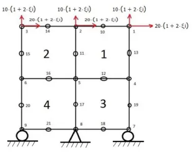
In order to test the implementation the simple 2D plane strain static elasticity problem shown in Figure2.3 was considered. It consisted of a simple assemblage of second order quadratic elements submitted to normal and tangential stresses. The problem was first solved with standard, displace-ment based finite eledisplace-ments available in ABAQUS and then with the user eledisplace-ment subroutine. An artificious damping coefficient ξ was used to introduced the imaginary components. A null value of this damping parameter recovers the classical solution. The problem was additionally solved manually.
Figure 2.3. Assemblage for static validation of the implemented user element subroutine.
In the case of a classical elastic material the generalized stress and strain tensors Σij = (σijR, σijI)
and Eij = (Rij, Iij) are related through the generalized constitutive tensorMijkl defined as follows
CHAPTER 2. USER ELEMENT SUBROUTINE 26
ˆ M =
λ+ 2µ λ 0 λˆ+ 2ˆµ λˆ 0 λ λ+ 2µ 0 λˆ ˆλ+ 2ˆµ 0
0 0 µ 0 0 µˆ
ˆ
λ+ 2ˆµ λˆ 0 −(λ+ 2µ) −λ 0 ˆ
λ λˆ+ 2ˆµ 0 −λ −(λ+ 2µ) 0
0 0 µˆ 0 0 −µ
(2.24)
and where ˆλ= 2ξˆiλ, ˆµ= 2ξˆiµ,λand µare the Lam´e constants from theory of elasticity,σij is the
Cauchy stress tensor and ij is the infinitesimal strains tensor.
The following set of complex loading was applied in the normal and tangential direction;
Px = 20(1 + 2ξˆi)
Py = 10(1 + 2ξˆi)
(2.25)
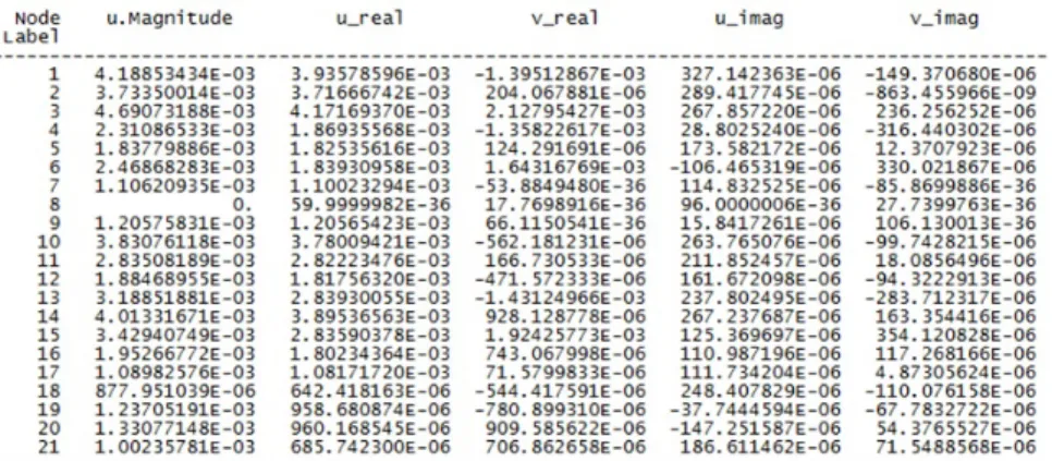
with ξ = 0.8, ˆν = 0.3(1.0 + 2ξˆi), ˆE = 210.000(1.0 + 2ξˆi). We solved the problem manually, with the implemented user element subroutine as initial validation and with classical real elements using ξ = 0. The results from the manual solution and those obtained with the ABAQUS user subroutine are reported in Figure 2.4 and 2.5.
CHAPTER 2. USER ELEMENT SUBROUTINE 27
Figure 2.5. Nodal displacements corresponding to the UEL solution.
On the other hand, the results obtained with a null value of the artificial damping parameter are exactly equivalent to the ones obtained with standard elements available in ABAQUS.
2.4.2
Scattering of Plane
P
waves by a Cylindrical Canyon in a
Half-Space
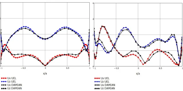
As a second verification example but now applied to a wave propagation problem, we solved the scattering of a P wave incident against a cylindrical canyon in a half-space. This problem has been previously solved by Kawase (1988) in the context of topographic effects in earthquake engineering, using a boundary integral equation formulation with half-space Green’s functions represented in the wave number domain. The problem has become a benchmark solution to validate numerical methods and to develop fundamental understanding of topographic effects in earthquake engineering. The geometry of the problem is shown in Figure 2.6. The characteristic dimension of the canyon corresponds to a radius a = 1.0Km. The mechanical properties of the half-space correspond to ρ = 1kg/m3, β = 1km/s and a Poissons ratio ν = 1/3. The
excitation consisted of a Ricker pulse of central frequency f c = 1.0Hz, maximum frequency f max= 4.0Hz and time durationT max = 8.0s applied at incidence angles (with respect to the vertical) corresponding to 0o and 30o . The analysis in the frequency domain was conducted with
a frequency step of ∆f =f max/32 . For the meshes were used 8-noded quadratic elements with characteristic dimensions satisfying theλc/10 criteria, where λcis the characteristic wavelength to
CHAPTER 2. USER ELEMENT SUBROUTINE 28
Figure 2.6. Finite element mesh for the semi-circular canyon.
Figure 2.7. Spatial distribution for the frequency domain transfer function over the canyon
surface for a dimensionless frequencyη= 1.0. The function corresponds to the amplitude of the
Chapter 3
The Problem of Site Effects in
Earthquake Engineering
Introduction
The frequency and spatial variations introduced by local topography on seismic ground motions are known to produce concentrated damage during earthquakes (e.g.,Northridge, California-1994; Kobe, Japan-1997; Kocaeli, Turkey-1999). In the theory of elastodynamics the quantification of these effects implies the solution of a wave scattering problem. Modern numerical techniques and the available computer power, has led to the possibility of realistic simulations of these effects for large scale regional domains, e.g.,(Bao et al.,1998;Okamoto et al.,2011;Taborda & Bielak,2011; Cupillard et al.,2012;Restrepo et al.,2012). At the same time, actual field records of large urban areas have become increasingly available during the last years providing additional evidence of the effects of topography. Despite these strong advances on the field, a detailed understanding of the underlying physics of the problem is still required.
In this chapter we address the problem of site effects in earthquake engineering from two point of views. In the first section of the chapter, we focus on the role played by the diffracted part of the motion on the modification induced by surface topographies. This idea is motivated by the fact, that in other problems related to propagation of acoustic and/or electromagnetic waves, the diffraction field has been clearly associated to the interaction of waves with geometric singularities. In earthquake engineering that idea has not been explored so far. In this work we use the numerical solution corresponding to the complete field and with the aid of the geometrical theory of raids we isolate the diffracted part of the motion. In particular we try to answer the question whether or not this part of the response capture the modifications induced by the site effects problem.
The second problem, related to the study of site effects, deals with the question of regional
CHAPTER 3. THE PROBLEM OF SITE EFFECTS IN EARTHQUAKE ENGINEERING 30
versus truly local effects. In particular, we try to answer the question of how important are the regional effects in the local response a given site. In order to explore an analysis approach to this problem we use a simple model of a canyon with the shape of a circular sector containing two localized regions with different material properties. We use our user element subroutines to address both problems where the frequency domain response is highly relevant. As analysis tool we proceed in a two-step algorithm taking as a starting point a method proposed by Professor’s Bielak group at Carnegie Mellon University originally formulated to save computer resources maintaining accuracy in the computations. That method has been called by its authors the domain reduction method as will be described later. In this work, since a different use is being made of the method we called it the modified domain reduction method.
3.1
The role of diffraction in the site effects problem
In this section we study the effects of topography on seismic ground motions, using a partition of the field into physically meaningful terms based upon the concept of diffracted motions. In earthquake engineering the terms scattering and diffraction have been used loosely as synonyms, Sanchez-Sesma & Iturraran-Viveros (2001), Mow & Pao (1971), however they are not. A strict definition of scattered field has been first attributed to Rayleigh: ”A scattered wave is the difference of the total wave field observed in the presence of an obstacle and the incident wave”. In the case of an obstacle being in a half-space, it is the difference of the total wave and the free field, Pao & Varatharajulu (1976). On the other hand, according to Keller (1962), diffracted waves are produced by incident waves which hit edges, corners or vertices of boundary surfaces or which graze such surfaces. This connection between the diffracted field and the geometric entities in the scatterer is expected to be reflected in the topographic effects.
The theory of diffraction has a long history. Its physical aspects have been studied in great detail, mainly in the context of electromagnetic waves. A landmark contribution and converted thereby in one of the building blocks for advancing the theory, is identified in the work of Som-merfeld (1896). He found the complete solution for the diffraction of electromagnetic plane waves by a semi-infinite crack in a homogeneous medium. Shortly after Sommerfeld’s work, MacDonald (1902) delivered the solution for the total field on a wedge, under plane and cylindricalSH waves. He wrote the total field as series expansions in terms of Bessel functions. A detailed study of Mac-donald’s solution, highlighting various aspects of the diffracted field can be found inSanchez-Sesma (1985).
CHAPTER 3. THE PROBLEM OF SITE EFFECTS IN EARTHQUAKE ENGINEERING 31
GTD is the introduction of diffraction coefficients, which upon application on the incident rays hitting the geometric singularity would deliver diffracted rays (e.g., just like reflection coefficients are used upon the incident field in a half-space). The diffraction coefficients in Keller’s work failed on the transition regions adjacent to shadow and reflection boundaries. This was later improved byKouyoumjian & Pathak (1974) who completed Keller’s GTD producing a workable expression to predict the diffraction by a generalized wedge.
Within the specific context of earthquake engineering, the particular contribution from the diffracted field to the total solution has not received much attention. In that area the problem has been traditionally solved in terms of the scattered field. A possible explanation may be due to practical reasons for both engineers and mathematicians and also, because of the lack of a sound theory of diffraction of mechanical waves. A particular reference to the role played by the diffracted field in the site effects problem can be found in the work of Sanchez-Sesma and its co-workers. For example in Sanchez-Sesma (1985) the author revisited Macdonald’s solution directly in the frequency domain. It was pointed out the fact that large differential motions were introduced by the diffracted field in the presence of shadow zones.
A partition of the field into incident, reflected and diffracted waves is also explicitly displayed by S´anchez-Sesma & Iturrar´an-Viveros (2001) in the study of diffraction of plane SH waves by a finite crack in a full space. They obtained a near field solution by superposition of two semi-infinite cracks of the Sommerfeld type. These authors explicitly isolated the diffracted field. Later Iturrar´an-Viveros et al. (2010) followed the same technique to find the solution for the diffraction by a cylindrical wave.
In contrast to the antiplane problem, in the case of in-plane waves the analytical solutions related to the diffracted field are just a few and the problem has been studied mainly from the numerical point of view. In this case complexities arise because of the coupling of boundary con-ditions and mode conversions at interfaces. One of the few particular solutions directly addressing diffraction is the one due toAchenbach (1973), who treated the problem of a semi-infinite slit un-der longitudinal waves obtained via integral transforms together with the Wiener-Hopf technique and the Cagniard-de-Hoop method. In the slit problem, the total field was shown to be composed of the incident P wave, reflected and diffracted P and SV waves and head waves connecting the diffracted P and SV fronts.
CHAPTER 3. THE PROBLEM OF SITE EFFECTS IN EARTHQUAKE ENGINEERING 32
In our treatment of topographic effects we obtain the diffracted field from the complete solution computed numerically. Our interest lies in establishing a connection between the topographic effect and the diffracted motions. For that purpose we study the two simple problems of cylindrical canyons of semi-circular and rectangular cross sectional shapes. Those two problems differ in the number of diffraction sources. Although from the very concept of diffraction it is clear that it is related to a geometric effect, the idea has seldom been explored in order to study the effect of topography on earthquake induced ground motions. The physically based partition provided by the diffracted field, is expected to reveal conceptual aspects of the response not evident in the traditional scattering approach. In this chapter we address the effects of topography on the incident ground motions using the diffracted field as a physical characterization of the site effects that directly links the geometry of the scatterer to the motion at a given receiver. The aim of this preliminary study is to contribute with the understanding of the topographic or site effects problem by proposing an alternative methodology to isolate the geometric effects and to suggest a partition of the field that can be used to isolate also the mechanical effects.
3.1.1
Prediction of the diffracted field
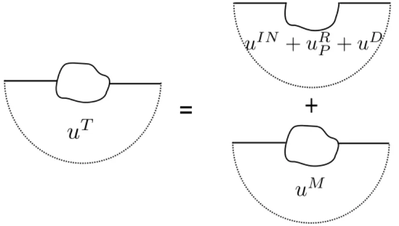
In the classical approach of the scattering problem, the solution is written as the contribution from the free field and the scattered motions, Pao & Varatharajulu (1976). However, while the free-field is well understood, the scattered motions are not. In problems involving arbitrary scattering surfaces, like canyons and ridges, an alternative physically sound way of studying the topographic effect is through the use of the concept of diffraction understood in the sense of optics. As described before, the diffracted motions correspond to that part of the response that cannot be predicted by geometrical methods. For example, if in a given problem the involved scattering surfaces are at least C2-continuous and fully illuminated, a complete, continuous solution, can be constructed based
on geometrical methods without formally solving the elastodynamics wave equation. However, if there are shadow zones or geometric singularities, the diffracted field is required in order to smooth out any discontinuities existing in the geometric field. Our proposed analysis method is based on this idea, where the total response is separated into the geometric and diffracted parts. In this way, a direct physical connection between the solution and the topographic features of the scatterer can be established in a source-receiver basis. In this section we describe these alternative partitions of the field and establish different relations between the involved terms. In particular we show how to obtain the diffracted field from the total displacement.
For the discussion that follows it is convenient to define the scattering problem with domain defined in Figure 3.1. It is composed of the homogeneous isotropic elastic-half space V0 with a
scatterer or topographic irregularityV1. The half-space and scatterer are assumed to be perfectly
coupled along the internal contact surface S. Similarly, SF = traction-free surface of the