The Next Generation Fornax Survey (NGFS) II The Central Dwarf Galaxy Population
19
0
0
Texto completo
(2) The Astrophysical Journal, 855:142 (19pp), 2018 March 10. Eigenthaler et al.. (dwarf) galaxy luminosity function.Another interpretation is that the large majority of low-mass DM halos have been very inefficient at star formation. It is now well established that dwarf galaxies are predominantly found in galaxy group and cluster environments, which tend to host dwarfs of differing morphological types. For example, while dwarf ellipticals (dEs) dominate the cluster galaxy population, star-forming dwarf irregulars (dIrrs) are most commonly found in the field or the cluster outskirts (Sandage & Binggeli 1984; Binggeli et al. 1985, 1988), suggestive of a link between dwarf galaxy evolution and the environment they reside in (e.g., Zhang et al. 2012; Mistani et al. 2016; Read et al. 2017; van de Voort et al. 2017). This morphology–density or morphology–distance relation for dwarf galaxies appears to be largely driven by tidal and ram pressure effects (Grebel et al. 2003). Dwarf galaxies have been detected throughout the Local Volume and beyond; see, for example, Binggeli & Cameron (1991), Côté et al. (1997), Karachentseva & Karachentsev (1998), Karachentseva et al. (1999), Karachentsev et al. (2000), Chiboucas et al. (2009), Müller et al. (2015), and many, many more.However, detections for the faintest dwarfs, the dwarf spheroidal galaxies, have so far been mainly limited to those within the Local Group (LG) due to their low surface brightness (e.g., McConnachie 2012).Thus, identifying and studying these faintest dwarf galaxy systems in nearby galaxy clusters and groups are crucial to constraining the ΛCDM cosmology. Previous observations seem to confirm the missing satellites problem when comparing the observed galaxy numbers with the ΛCDM halo mass function in environments covering a range of galaxy densities (e.g., Pritchet & van den Bergh 1999; Trentham & Tully 2002; Ferrarese et al. 2016; Taylor et al. 2017), including rich galaxy clusters. Potentially easing some of this tension is the discovery in recent years of ultrafaint dwarf (UFD) and dwarf spheroidal (dSph) satellites throughout the Local Group (Willman et al. 2005; Belokurov et al. 2006, 2007, 2010, 2014; Zucker et al. 2006a, 2007; McConnachie et al. 2009; McConnachie 2012; Bechtol et al. 2015; Drlica-Wagner et al. 2015; Koposov et al. 2015; Laevens et al. 2015; Homma et al. 2016) and rich dwarf galaxy systems around nearby giant galaxies and clusters (Karachentsev et al. 2007; Müller et al. 2015, 2017; Muñoz et al. 2015; Crnojević et al. 2016; Ordenes-Briceño et al. 2016; Sánchez-Janssen et al. 2016). The newly discovered UFDs appear to be an extension of dSphs to lower luminosities (e.g., Muñoz et al. 2015), being much fainter (MV −8 mag) and smaller (reff300 pc) than classical dSphs.UFDs have luminosities comparable to globular clusters (GCs), which are much more compact (re10 pc). Classical GCs typically have M/LV≈2 (e.g., McLaughlin & van der Marel 2005; van de Ven et al. 2006; Baumgardt et al. 2009; Strader et al. 2011; Taylor et al. 2015), whereas, in contrast, UFD kinematics reveal M/LV100, indicative of DM-dominated systems (e.g., Kleyna et al. 2005; Simon & Geha 2007). In addition to the rich populations of low surface brightness (LSB) dwarf galaxies in the Local Volume, there have also been discoveries of ultradiffuse galaxies (UDGs), first found and described by Sandage & Binggeli (1984), Impey et al. (1988), Ferguson & Sandage (1988), and Bothun et al. (1991). More recent discoveries of this galaxy class have been identified in various galaxy aggregates like the Coma and Virgo galaxy clusters (Koda et al. 2015; Mihos et al.. 2015; van Dokkum et al. 2015a), the Pisces–Perseus supercluster (Martínez-Delgado et al. 2016), a galaxy group (Merritt et al. 2016), in the galaxy cluster Abell 2744 (Janssens et al. 2017) and Abell 168 (Román & Trujillo 2017a), and even outside of groups and clusters (Román & Trujillo 2017b). The low stellar masses (∼6 × 10⁷ Me) and large radii (1.5–4.6 kpc) of UDGs result in very low surface brightness values in the range μ0,V≈26–28.5 mag arcsec−2, making them challenging to detect. The existence of this mysterious new galaxy class in mostly dense galaxy cluster environments prompts the obvious question of whether there might be similar populations in other galaxy aggregates, or whether they are reserved for rich galaxy clusters only. In the present work, we attempt to address these questions by investigating the properties of the low surface brightness dwarf galaxy population in the inner region of the Fornax galaxy cluster, one of the most nearby southern galaxy clusters, using data obtained as part of the Next Generation Fornax Survey (NGFS). The survey constitutes of deep, wide-field, multipassband u′g′i′ observations taken with the Dark Energy Camera (DECam; Flaugher et al. 2015) mounted on the 4 m Blanco telescope at Cerro Tololo Interamerican Observatory (CTIO). Given its proximity, Fornax is a goldmine for studying the formation and evolution of galaxies and other stellar systems, such as GCs and dwarf galaxies, in a galaxy cluster environment (Muñoz et al. 2015; Iodice et al. 2016; D’Abrusco et al. 2016; Wittmann et al. 2016).Compared to its northern counterpart, the Virgo cluster, Fornax has twice the central galaxy density, half the velocity dispersion, and accordingly a distinctly lower mass (7 ± 2×10¹³ Me; Ferguson 1989; Schuberth et al. 2010). Furthermore, the core of Fornax is dynamically more evolved (Churazov et al. 2008), and its early-type (E/S0) galaxy fraction is significantly larger (∼50%) than that of Virgo (∼35%), considering member galaxies brighter than MB=−16 mag not classified as dwarfs in the Fornax Cluster Catalog (FCC; Ferguson 1989) and VCC (Binggeli et al. 1985) catalogs. Noting the above, the Fornax cluster is an excellent target to study faint baryonic substructures in one of the most nearby cluster environments. Throughout this work, we utilize a distance modulus of 31.51±0.03 mag for Fornax, corresponding to a distance of ∼20 Mpc (Blakeslee et al. 2009). Derived magnitudes refer to the AB system. 2. Observations Our imaging is conducted as part of the NGFS, for which we provide an abbreviated summary here to put the present contribution into context. The NGFS is an ongoing survey of the Fornax galaxy cluster core in the optical u′, g′, and i′ and the near-infrared (NIR) J and Ks filters, targeting the inner 30 deg2, corresponding to ∼1 Mpc in galactocentric radius centered on the cD galaxy NGC 1399.Here we focus on the NGFS optical survey observations, which consist of nine contiguous DECam tiles (see Figure 1), each aiming at a minimum point-source detection limit of u′=26.5, g′=26.1, and i′=25.3 mag at S/N=5 over the point-spread function (PSF) area. With the goal of maximizing sensitivity to LSB structures in the imaging, we employ the Elixir-LSB dithering technique developed for the complementary Next Generation Virgo Survey (NGVS; see Ferrarese et al. 2012, for details), and we use raw images processed by the DECam Community Pipeline (CP; v.2.5.0 Valdes et al. 2014) to produce fully 2.
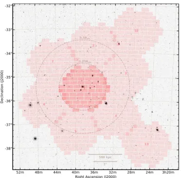
(3) The Astrophysical Journal, 855:142 (19pp), 2018 March 10. Eigenthaler et al.. 3. Analysis 3.1. Detection of LSB Dwarf Galaxies To detect LSB dwarf galaxy candidates, we first constructed RGB images from the observed u′g′i′ frames to take advantage of the total flux captured in each passband while preserving color information.We then visually inspected these frames, looking explicitly for diffuse LSB galaxies.The RGB images allow us to easily identify dwarf galaxy candidates by considering their colors, sizes, and overall morphologies (e.g., comparatively flat surface brightness profile and nucleation). We also included LSB galaxies having SF knots or blue colors, not specifically selecting against these sources. While automated algorithms can prove very effective in detecting faint galaxies (NGVS paper, Ferrarese et al. 2016), for the purpose of this work, we present a by-eye classification done independently by several people. The advantage of this method over automated algorithms like SE is obvious. For example, SE is only able to analyze one frame–passband combination at a time and often fails to detect extended LSB sources due to contamination by foreground stars, while visual inspection allows for the identification of galaxy candidates based on all aforementioned criteria simultaneously.We find that galaxy color is particularly effective in this regard since the colors of cluster dwarfs are expected to follow a cluster red sequence as seen in many galaxy aggregates (Gladders & Yee 2005; Roediger et al. 2017), with likely origins in the galaxy mass–metallicity relation. Combining this criterion with the diffuse morphologies arising from shallow dwarf surfacebrightness profiles results in a straightforward detection strategy for dwarf galaxy candidates.Despite these advantages, the disadvantage of visual inspection is that it precludes us from quantifying a selection function to verify sample completeness and that it has the potential to introduce human bias.Hence, to avoid any personal detection biases, we (P.E., T.H.P., Y.O., M.A.T., K.A.M., K.X.R.) individually investigated the RGB images independently, yielding up to six separate dwarf galaxy candidate catalogs for each tile. Tile 1 has five independent candidate catalogs.. Figure 1. Overview of the NGFS mosaic footprint consisting of DECam tiles 1–7, 10, and 13, with the central tile investigated in this work being highlighted.The dashed circles indicate a quarter and a half virial radius, i.e.,0.25 and 0.5 Rvir.The underlying figure is taken from DSS1 obtained via the Online Digitized Sky Surveys server at the ESO Archive.The displayed field is 7°×7°.. calibrated image stacks. The CP processes the raw DECam images for basic calibration steps (e.g., bias correction, flatfielding, image crosstalk correction), and we use the ASTRO18 MATIC software suite (SOURCE EXTRACTOR, hereafter SE, v.2.19.5; SCAMP, v.2.0.1; SWARP, v.2.38.0; Bertin & Arnouts 1996; Bertin et al. 2002; Bertin 2006) to perform the astrometric and photometric calibrations based on reference stars from the 2MASS Point Source Catalog (Skrutskie et al. 2006) and SDSS stripe 82 standard star frames, respectively, to build our image stacks. We then apply our custom background subtraction strategy based on an iterative masking and sky modeling procedure. We cross-validated our u′g′i′ photometry by running PSF photometry in the surveyed area and comparing the resulting magnitudes with the U, B, V, and I photometry of Kim et al. (2013) for globular clusters in the same field.In order to adequately compare the two photometries, we utilized the empirical transformation equations from Jordi et al. (2006) and found good agreement within the uncertainties. In a previous contribution (Muñoz et al. 2015), we presented a preliminary i′-band-based analysis of a rich population of dwarf galaxies in the central ∼3 deg2 tile of the NGFS footprint.Here we build upon these results by including the full u′g′i′ color information for the central dwarf galaxy population with an average seeing of 1 7 in u′, 1 3 in g′, and 1 1 in i′. In order to evaluate the detection threshold for extended sources in u′, g′, and i′, we directly measured the pixel statistics on the sky in the individual passbands, resulting in 1σ surface brightness limits of μu′=28.04, μg′=29.06, and μi′=28.15.Figure 2 illustrates the footprint of the central NGFS tile. 18. 3.2. Quality Flags To estimate the reliability of our detections, we match the catalogs using TOPCAT (Taylor 2005) to quantify in how many catalogs a given source was found.We then assign quality flags to each dwarf galaxy candidate such that one found in all five catalogs is assigned a flag , in four catalogs a flag , and so on.The matching is done systematically so that we first match all flag objects and remove them from the corresponding catalogs.We continue by searching for flag sources, and we continue until all remaining sources are flag , that is, untrustworthy candidates only identified by a single team member. In order to find all matches for a given flag k, all 5 possible k catalog combinations have to be matched, leading to lists of 145 flag , 59 flag , 54 flag , 29 flag , and 136 flag sources. Figure 3 shows the distribution of quality flags, which illustrates the potential human detection bias given the large number of accumulated flag sources present in the merged candidate catalog.Conversely, those sources with multiple independent identifications, flags , show a strong trend toward unanimous detections. Flag illustrates the average. (). http://www.astromatic.net/software. 3.
(4) The Astrophysical Journal, 855:142 (19pp), 2018 March 10. Eigenthaler et al.. Figure 2. Spatial footprint of the central NGFS tile centered on NGC1399 and analyzed in this paper (shown in white).The distribution of the dwarf galaxy population corresponds to the one listed in Table 1. Both bright galaxies (MB −16; orange) and dwarfs (red) are indicated, and the two brightest galaxies are labeled with their NGC numbers. Ellipticities and position angles of the symbols are scaled by the corresponding GALFIT model values.The dashed circle indicates 0.25Rvir of the Fornax cluster (Rvir = 1.4 Mpc), as determined by Drinkwater et al. (2001).. number of sources uniquely identified by one person (solid line) as well as all accumulated sources (dashed line). The lower panel in Figure 3 shows the correlation between detection flags and median values of galaxy apparent g′-band magnitude, effective radius (re), and surface brightness (μg′) for each flag. As expected, apparent magnitude and re show clear trends toward brighter and larger galaxies having flags , while flags correspond to fainter and smaller sources. No obvious correlation is seen with μg′.We note that these correlations should be taken with caution, since we only measure structural parameters for a small subsample of flags. Moving forward, we consider only galaxies with detection flags , that is, with at least three independent identifications, to be dwarf galaxy candidates, yielding a final sample of 258 sources. Of these candidates, 75 (∼29%) show evidence of nucleation based on visual inspection of the u′-, g′-, and i′-band images, while 183 galaxies (∼71%) show no nucleus. 3.3. Comparison with Existing Catalogs. Figure 3. Dwarf galaxy candidate detection flags. Upper panel: distribution of detected dwarf galaxy candidates as a function of the quality flags. For flag , the solid line indicates the average number of sources uniquely identified by one person, while the dashed line shows all accumulated flag objects. Lower panel: total galaxy magnitudes (red), surface brightness (yellow), and effective radii (blue) as a function of quality flags. Sources with flags are considered dwarf galaxy candidate detections. See text for details.. We compare our sample with galaxies flagged as likely members in the FCC (Ferguson 1989).Out of 340 FCC galaxies, 112 fall in our observed DECam footprint.We note that we could not reidentify FCC 162, which is reported to be located within the halo of the bright elliptical NGC 1379 4.
(5) The Astrophysical Journal, 855:142 (19pp), 2018 March 10. Eigenthaler et al.. (FCC 161), leaving 111 recovered FCC galaxies. Of these, 90 are fainter than MB=−16 mag and, hence, can be considered as dwarf galaxies (Ferguson & Binggeli 1994; Tammann 1994). In addition, two galaxies with MB−16 (FCC 136 and FCC 202) have explicitly been classified as dwarfs in the FCC catalog, resulting in a total number of 92 FCC dwarfs in our observed footprint. We also recover 45 galaxies from the Mieske et al. (2007) catalog that have not been classified as FCC galaxies. Finally, we checked for Mieske et al. (2007) dwarfs that are not in our sample and conclude that, based on their morphologies and colors, all are likely to be background galaxies. Summarizing, we find a sample of 258 – 92 – 45=121 previously uncataloged dwarf candidates. We note that this number is smaller than in our recent publication (see Muñoz et al. 2015), since in the present work we only consider galaxies with quality flags as dwarf identifications. Figure 2 shows a schematic representation of the spatial distribution of the detected dwarf galaxy candidates and known bright galaxies in the central DECam tile of the NGFS footprint analyzed in this work (tile 1 in Figure 1). The symbol shape, alignment, size, and opacity of each galaxy marked in Figure 2 are scaled by the corresponding ò, PA, re, and Mg, respectively, as obtained from our GALFIT models. We point out that since precise 3D spatial information is not known, Mg may vary by up to ∼0.16 mag due to the unknown depth of the cluster.19. between the four resulting model fits for each galaxy, we obtain a qualitative estimate of the robustness of a fit. In the best scenario, all initial guesses converge to the same solution, but in most cases two or three initial guesses converge to a single model, leaving one or two outliers. In the worst cases, all initial guesses yield different results.To properly assess the reliability of the fits, we compare the galaxy, model, and residual images for each dwarf in detail. In most cases where multiple initial guesses converge to the same result, visual inspection shows the fits to be reliable. In the second iteration, we consider galaxies for which the automatic fitting procedure did not converge to a common solution, due to their diffuse natures or small extents. For these galaxies—the majority of our sample—the models display a severe mismatch with respect to the surface brightness distributions of the galaxies, or the residual images show signs of oversubtraction. We refine the fitting procedure for these galaxies as follows. First, we estimate the total galaxy luminosity by running SE on the galaxy postage stamp images and use the resulting MAG_AUTO values from the corresponding segmentation as initial guesses for the GALFIT Sérsic models. Keeping these values fixed reduces the number of free parameters available for the next galaxy model, stabilizing the fit and resulting in more robust estimates of the remaining model parameters. We then use the new parameters and fix them and allow GALFIT to recompute the galaxy luminosity freely. In the final step, the newly determined galaxy magnitude was again fixed, and we recompute the other parameters, resulting in model parameters that are all consistently derived by GALFIT. In this way, all nonnucleated dwarfs are fit successfully, leaving little to no sign of the galaxies’ light in the residual images (see Figure 4).. 3.4. Surface Brightness Profile Modeling We determine the structural parameters for the 258 dwarf candidates in u′, g′, and i′ filters utilizing the software package GALFIT (v3.0.5; Peng et al. 2010). GALFIT is an effective tool for extracting structural information from dwarf galaxies, allowing the user to model the two-dimensional distribution of the diffuse starlight in galaxies with numerous parametric functions.Utilizing the full 2D information for a given galaxy enables us to obtain reliable fits to the surface brightness distribution constrained by each nonmasked image pixel. Surface brightness profiles of dwarf galaxies are commonly well fit by a single-component Sérsic (1968) model: I (r ) = Ie exp {- bn [(r re )1. n. - 1]},. 3.4.2. Fitting Nucleated Dwarfs. We modify the above strategy for dwarf candidates that show evidence of nucleation in order to account for the excess light at their centers.While in principle a two-component model consisting of a King (1962) profile for the nucleus and a Sérsic profile for the spheroid would be preferred, the pixelscale sizes of the nuclei preclude this approach.Very few stable solutions are found for the nuclei, and the addition of model parameters increases the likelihood of degenerate solutions, making this approach futile. As a solution to this problem, for a given nucleated candidate, we instead mask the nucleus and fit a single Sérsic model to the diffuse spheroid iteratively. We first manually create a preliminary mask for the nucleus in the segmentation maps and use it to fit the galaxy light without the nuclear component. From the resultant residual images (including the nucleus), we generate an improved mask for the nucleus and any other sources contaminating the diffuse components of the dwarfs. We then repeat the fit using the improved mask and iteratively improve the mask and residual image. If the nucleus is not masked correctly, the Sérsic model will attempt to fit it partially, thus predicting a too-high n and producing symmetric regions of over- and undersubtraction in the residuals. Following this procedure, we find that three to four iterations result in clear nucleus–spheroid separation free of symmetric residuals in the circumnuclear regions, and give stable solutions for the spheroid components of all nucleated dwarf candidates confirmed by visual inspection.. (1 ). which is parameterized by the effective radius re, the intensity Ie at re, and the shape index n (also referred to as the Sérsic index) that defines the curvature of the model. The parameter bn is linked to n such that half of the total light from the model is enclosed within re (Caon et al. 1993). We choose this singlecomponent, ellipsoidal model to measure the global morphology of our dwarf galaxy candidates. Our iterative fitting procedure is split into several steps. First we create postage stamp images for each dwarf candidate in the u′-, g′-, and i′-band frames and construct corresponding segmentation maps using SE. The segmentation maps are used to create bad-pixel masks for each dwarf, masking any nondwarf sources above a 2σ threshold. This initial step results in dwarf-only images that are used for subsequent model fits. 3.4.1. Automatic and Refined Fitting. In a first iteration, we fit galaxies assuming four different initial guesses for the Sérsic model parameters. By comparing 19. This applies only under the assumption of spherical symmetry.. 5.
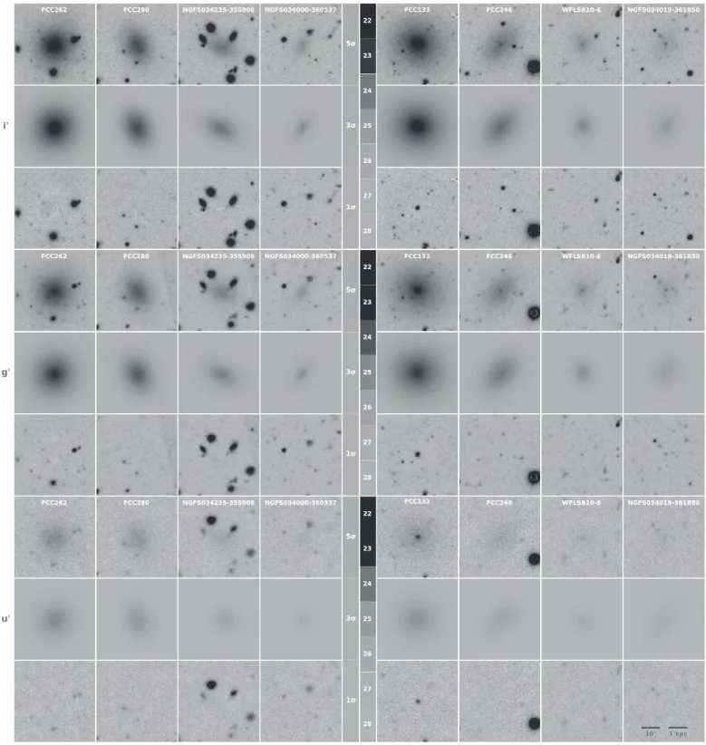
(6) The Astrophysical Journal, 855:142 (19pp), 2018 March 10. Eigenthaler et al.. Figure 4. Examples of the dwarf galaxy surface-brightness modeling with GALFIT. Four nonnucleated (left) and four nucleated (right) dwarfs with successively decreasing (left to right) effective surface brightness values are shown in u′ (lower panels), g′ (middle panels), and i′ (upper panels) as examples. We show the dwarf galaxy postage stamps, the corresponding 2D Sérsic (1968) models, and residual images (galaxy–model) for every passband. The grayscales show values of constant surface brightness ranging from μ=22 to 28 mag arcsec−2 in steps of 1 mag arcsec−2 as well as 1σ, 3σ, and 5σ surface-brightness detection thresholds in all passbands.Note that only the spheroid component is modeled for nucleated dwarfs so that the nuclear star cluster is visible in the residual images. We also point out the clear variance in the nucleus-to-galaxy luminosity ratio for these dwarfs. Dwarfs are, from left to right, FCC262, FCC280, NGFS034235-355906, NGFS034000360537, FCC133, FCC246, WFLSB10-6, and NGFS034019-361850. The images cover 0.72′ (∼4.25 kpc) on a side.. Figure 4 shows models for eight (four nonnucleated and four nucleated) representative dwarf galaxies with successively decreasing average surface brightness in the range 24.0 μi′/mag26.5. A comparison of the galaxies (top row), models (middle row), and residuals (bottom row) clearly. illustrates the robustness of our modeling approach. In total, we derive structural properties for 246/258 (95%) of the detected dwarf candidates in the i′ and g′ bands, dropping to 144 (56%) in the u′ band. While the lower fraction of modeled galaxies in the u′ band is likely due to the lower sensitivity and 6.
(7) The Astrophysical Journal, 855:142 (19pp), 2018 March 10. Eigenthaler et al.. Table 1 Photometric Properties and Stellar Masses of the Dwarf Galaxy Sample ID. Referencea. NGFS033309-352349 NGFS033311-353956 NGFS033348-355010 NGFS033350-355706 NGFS033400-354533 NGFS033406-351638 NGFS033407-352838 NGFS033409-353100 NGFS033412-351343 NGFS033414-354910 NGFS033423-355042 NGFS033427-350621 NGFS033433-350236 NGFS033436-360315 NGFS033443-353115 NGFS033446-345334 NGFS033456-351127 NGFS033458-351324 NGFS033458-350235 NGFS033500-351920. FCC114 K FCC125 K K FCC127 K FCC130 FCC131 K K K K K K K FCC140 WFLSB6-2 FCC142 FCC144. α (J2000) 03h33m08 03h33m10 03h33m48 03h33m49 03h33m59 03h34m05 03h34m06 03h34m09 03h34m12 03h34m14 03h34m23 03h34m27 03h34m32 03h34m36 03h34m43 03h34m46 03h34m56 03h34m57 03h34m58 03h35m00. δ (J2000) 63 93 42 87 75 97 97 18 13 29 34 18 55 38 39 06 41 56 19 20. −35°23′49 −35°39′56 −35°50′09 −35°57′06 −35°45′33 −35°16′38 −35°28′37 −35°30′59 −35°13′43 −35°49′10 −35°50′41 −35°06′20 −35°02′35 −36°03′15 −35°31′15 −34°53′33 −35°11′27 −35°13′24 −35°02′34 −35°19′20. 01 16 66 17 26 25 99 50 28 05 89 76 50 27 07 56 42 42 80 26. i′ (mag). g′ (mag). u′ (mag). (g′−i′)0 (mag). (u′−g′)0 (mag). (u′−i′)0 (mag). M gb (mag). log (Me). 18.67 20.05 17.64 20.91 18.30 18.61 20.63 17.38 19.15 19.79 19.18 20.55 20.38 20.56 20.45 20.52 17.61 18.72 17.34 18.24. 19.57 21.62 18.50 21.57 19.52 19.39 22.47 18.10 19.92 20.47 20.51 21.55 20.62 21.61 21.04 21.29 18.25 19.72 18.37 19.11. 20.28 K 19.64 K 20.05 20.30 K K 20.50 K K K K K K K 19.37 20.45 19.45 19.83. 0.90 1.57 0.86 0.66 1.22 0.78 1.84 0.72 0.77 0.68 1.33 1.00 0.24 1.05 0.59 0.77 0.64 1.00 1.03 0.87. 0.72 K 1.15 K 0.54 0.92 K K 0.59 K K K K K K K 1.12 0.74 1.08 0.73. 1.62 K 2.01 K 1.76 1.70 K K 1.36 K K K K K K K 1.76 1.74 2.11 1.60. −11.94 −9.89 −13.01 −9.94 −11.99 −12.12 −9.04 −13.41 −11.59 −11.04 −11.00 −9.96 −10.89 −9.90 −10.47 −10.22 −13.26 −11.79 −13.14 −12.40. 7.11 7.05 7.62 6.24 7.27 7.17 6.96 7.68 6.88 6.70 7.28 6.56 6.23 6.58 6.39 6.45 7.59 7.11 7.74 7.28. Notes. a Reference to galaxies listed in the FCC catalog (Ferguson 1989) and in Mieske et al. (2007). b Assuming a distance modulus of (m − M)0=31.51 mag (Blakeslee et al. 2009). (This table is available in its entirety in machine-readable form.). comparatively low flux of galaxies in this particular passband, the 12 missing galaxies in the i′ and g′ bands are either too faint or too strongly contaminated by a bright nearby star.We list our photometric results in Table 1, including galaxy coordinates, all available total galaxy magnitudes derived from GALFIT, integrated galaxy colors, absolute g′-band magnitudes (Mg′), and estimated total stellar masses ( ; see also Section 4.3).We also list the cross-identifications from the FCC and the Mieske et al. (2007) catalogs. Likewise, we list in Table 2 all available structural parameters derived by GALFIT in this work, also indicating for each galaxy whether or not a nucleus is present.. áreñu ¢ = 0.69 0.03 kpc, which is at first impression indicative of a lack of significant stellar population gradients in the spheroid components. We find in all filters similar minimum drop-offs in re and similar re, max≈2 kpc. However, the re consistency plots in the bottom panels show that the u′-band half-light radii are systematically smaller than in the redder bands. This may be due to the lower surface brightness depth of our u′-band data or to stellar population gradients pointing toward bluer cores of dwarf galaxy spheroids.Quantitatively evaluating the detailed causes of this intriguing result goes beyond the scope of this paper. We will, however, return to this aspect in a future paper on the stellar population content of the NGFS dwarf galaxies. The distributions of Sérsic indices n closely follow Gaussian profiles in all passbands with similar mean values of ánñu ¢ = 0.83 0.03, ánñg ¢ = 0.78 0.02, and ánñi ¢ = 0.83 0.02. However, we note that there may be an observational bias giving rise to the narrow distributions in n, likely due to selection effects since we explicitly looked for diffuse galaxies in our search for dwarf galaxy candidates. We find generally more platykurtic distributions in ò and PA than in re and n.Our measurement values are in the range 0.0ò0.7, with indications that ò may be bimodally distributed.Despite the visual impression, detailed Gaussian mixture modeling does not conclusively quantify whether a single-mode or a bimodal distribution is preferred.We find a marginal tendency of increasing average ellipticity toward bluer passbands. Interestingly, we do not find any highly elongated dwarfs, with 97% of the NGFS dwarfs exhibiting ellipticities ò<0.55. This is in very good agreement with the result from SánchezJanssen et al. (2016) for dwarfs in the core of the Virgo cluster, and with the fast rotators in the ATLAS3D sample (Cappellari 2016). Finally, we see that position angles do not show any. 4. Results 4.1. Structural Parameters We show in Figure 5 the distribution functions of the structural parameters derived by GALFIT for the entire dwarf galaxy sample in the u′, g′, and i′ filters.The upper panels show the distributions of effective radius (re), Sérsic profile shape parameter (n), ellipticity (ò), and position angle (PA), split by filter with u′ in the top row followed by g′ and i′ below.The histogram bin widths were chosen based on Knuth’s rule (Knuth 2006).Alternative visualizations of the distributions are shown by the solid relations, which are nonparametric Epanechnikov kernel probability density estimates (KDEs) for each parameter–filter combination. The lower panels show consistency plots for each structural parameter, as derived from the u′, g′, and i′ filters. While re and n show well-defined peaks in their distributions, the ò and PA values are more broadly distributed. We find a characteristic effective radius consistent between the passbands in the range 0.1 re kpc 2.0 with a similar mean size of áreñg ¢ = 0.68 0.02 kpc , áreñi ¢ = 0.71 0.03 kpc, and 7.
(8) The Astrophysical Journal, 855:142 (19pp), 2018 March 10. Eigenthaler et al.. Table 2 Structural Properties of the Dwarf Sample ID NGFS033309-352349 NGFS033311-353956 NGFS033348-355010 NGFS033350-355706 NGFS033400-354533 NGFS033406-351638 NGFS033407-352838 NGFS033409-353100 NGFS033412-351343 NGFS033414-354910 NGFS033423-355042 NGFS033427-350621 NGFS033433-350236 NGFS033436-360315 NGFS033443-353115 NGFS033446-345334 NGFS033456-351127 NGFS033458-351324 NGFS033458-350235 NGFS033500-351920. Reference FCC114 K FCC125 K K FCC127 K FCC130 FCC131 K K K K K K K FCC140 WFLSB6-2 FCC142 FCC144. i′. Typea d d d d d d d d e d d d d d d e e d e d. g′. u′. reb. nc. òd. PAe. reb. nc. òd. PAe. reb. nc. òd. PAe. 0.699 0.883 0.896 0.435 0.563 0.619 0.623 1.819 0.526 0.634 0.848 0.466 0.499 0.573 0.377 0.440 0.898 0.559 1.011 0.597. 0.81 0.63 0.71 0.45 0.87 0.82 0.82 0.80 0.75 0.39 0.73 0.95 0.78 0.62 0.74 0.65 0.81 1.00 1.34 0.81. 0.43 0.24 0.15 0.39 0.24 0.23 0.13 0.17 0.44 0.17 0.21 0.42 0.36 0.51 0.09 0.29 0.46 0.29 0.06 0.23. 98 125 141 114 21 72 173 135 127 2 98 26 100 168 99 140 95 41 134 56. 0.642 0.757 0.866 0.503 0.421 0.602 0.359 2.008 0.521 0.715 0.673 0.356 0.657 0.467 0.400 0.410 0.968 0.508 0.847 0.592. 0.72 0.23 0.65 0.50 0.63 0.82 0.30 0.91 0.91 0.57 0.41 0.68 0.69 0.50 0.73 0.67 0.89 0.80 1.02 0.77. 0.47 0.50 0.14 0.43 0.17 0.22 0.16 0.18 0.47 0.25 0.15 0.32 0.39 0.36 0.11 0.22 0.47 0.31 0.06 0.25. 97 106 139 136 30 74 118 130 128 179 69 33 99 179 89 98 94 50 149 56. 0.584 K 0.766 K 0.622 0.526 K K 0.475 K K K K K K K 0.795 0.486 0.708 0.523. 0.64 K 0.50 K 1.13 0.76 K K 0.72 K K K K K K K 0.63 0.65 0.92 0.82. 0.46 K 0.13 K 0.30 0.24 K K 0.34 K K K K K K K 0.47 0.30 0.11 0.23. 99 K 150 K 29 73 K K 109 K K K K K K K 94 54 16 55. Notes. a Morphological galaxy type classification: e=nucleated, d=nonnucleated dwarf galaxy. b Effective radii given in kpc. c Sérsic index (Sérsic 1968; Caon et al. 1993). d Ellipticity ò=1−b/a. e Position angle in ° from north toward east. (This table is available in its entirety in machine-readable form.). preferred alignment and populate the whole parameter range 0°PA180° with very good consistency between the u′, g′, and i′ filters. The lower panels in Figure 5 compare the derived structural parameters in all three passbands. Assuming the galaxies are homologous in all passbands, that is, the same re, n, ò, and PA, one would expect all galaxies to follow unity, with the observed scatter arising from the statistical uncertainties of the measurements. However, this would also imply that the dwarf candidates do not exhibit color gradients, which is not necessarily true, as pointed out above. Hence, while the statistical measurement errors likely contribute to the observed scatter, intrinsic differences between galaxy models—such as color gradients—may also play a role. In general, the i′- versus u′-band comparison shows a systematically larger scatter than that of the i′ versus g′ bands, in part likely due to the shallower u′-band observations. Detailed consideration of the derived R2 values reveals that re and PA show the tightest correlations, implying that these structural parameters constrain the galaxy models most efficiently in either of the filters. Meanwhile, the n distribution shows a much larger deviation from unity, indicating that it is more difficult for GALFIT to find one unique solution for the Sérsic index in all passbands. In any case, we note that the range in n is relatively small:83% of the measured galaxies have shape parameters in the range 0.5n1.5, and variations on the order of Dn 0.1 are expected. We also highlight the nucleated dwarfs in the parameter distributions of the upper panels of Figure 5, which clearly show that the average spheroid of a nucleated dwarf has a larger half-light radius and more spherical light distribution,. with a hint of a slightly more exponential-type Sérsic profile (i.e., n closer to 1) than their average nonnucleated counterpart. There is mild indication that the spheroid components of nucleated dwarf galaxies are more spheroidal, that is, show lower ellipticity, than their nonnucleated counterparts. Except for effective radii, the nucleated dwarf samples show tighter correlations than the overall samples in the filter correlation plots. This is primarily because the nucleated dwarfs are on average brighter than nonnucleated dwarfs. We find that the nucleation fraction (nuc ) is a strong function of galaxy luminosity, and nuc shows a strong tendency toward higher fractions in bins containing the brightest galaxies and declines to ∼0% when only the faintest galaxies are considered. Likewise, the cumulative nuc shows a similar trend, in that nuc = 100% for exclusively bright galaxies and falls to the final value of ∼29% for the overall dwarf galaxy sample. The same trend of higher nucleation fractions in brighter dEs was found in the Virgo cluster by Grant et al. (2005) and Lisker et al. (2007), indicating a possibly generally valid trend. We furthermore note that, given the present seeing, low-luminosity nuclei that have low contrast with the host galaxy could remain unidentified and affect the derived nucleation fraction. 4.2. Color–Magnitude Relations Color–magnitude diagrams (CMDs) of galaxies have long been used to infer the mass assembly and star formation histories of galaxies in large-area, deep surveys with ground and space-based telescopes (e.g., Baldry et al. 2004; Bell et al. 2004, 2012; Faber et al. 2007; Trayford et al. 2016; Roediger et al. 2017).Multipassband CMDs are powerful tools to obtain 8.
(9) The Astrophysical Journal, 855:142 (19pp), 2018 March 10. Eigenthaler et al.. Figure 5. Structural parameters derived from GALFIT in the u′, g′, and i′ filters. Upper panels: distributions for the effective radius (re), Sérsic profile shape parameter (n), ellipticity (ò), and position angle (PA) in all three passbands. Lighter histograms refer to nucleated dwarfs only. Smooth curves show the corresponding Epanechnikov kernel probability density estimates for the entire sample (solid) and nucleated dwarfs only (dashed). Vertical lines indicate the mean (lighter) and median (darker) of the overall distributions for the entire sample of dwarf galaxies (solid lines) and nucleated dwarf only (dashed lines). Lower panels: comparison of u′- and g′-band parameters as a function of the corresponding i′-band values. Straight lines show the unity relations. Symbols with black dots refer to nucleated dwarfs. Correlation coefficients R2 are shown in each panel for both the overall sample and the nucleated dwarfs only.. reaches down to stellar masses of ∼106 Me, while the optical g′- and i′-band photometry reaches even lower values.All three panels clearly illustrate the expected red sequence for early-type cluster galaxies, where brighter systems exhibit redder colors than fainter ones.This color–magnitude relation of galaxies is commonly interpreted as a mass–metallicity relation since the deeper potential wells of more massive galaxies more easily retain metals produced throughout their star formation history (e.g., Kodama & Arimoto 1997; Poggianti et al. 2001; Tremonti et al. 2004; Savaglio et al. 2005; Baldry et al. 2008; Maiolino et al. 2008; Møller et al. 2013; Segers et al. 2016; Ma et al. 2016). We fit linear relations to the CMDs of NGFS dwarfs and derive shallow color gradients in the sense of D (g¢ - i¢)0 Dg¢= (g ¢- i ¢)0 = -0.01, D (u¢ - g¢)0 Dg¢ = (u ¢- g ¢)0 = -0.09, and D (u¢ - i¢)0 Dg¢ = (u ¢- i ¢)0 = -0.13.. constraints of luminosity-weighted average stellar population ages and metallicities, as well as stellar masses of large samples of galaxies (e.g., Chilingarian & Zolotukhin 2012). In the left panels of Figure 6 we show the (g′ − i′)0, (u′ − g′)0, and (u′ − i′)0 versus g′ CMDs for NGFS dwarf galaxies and compare them with other galaxy samples and theoretical predictions of color–magnitude relations.We account for foreground extinction toward Fornax by utilizing average extinction coefficients (Au′, Ag′, and Ai′) derived from several bright Fornax galaxies based on the recalibrated extinction maps of Schlafly & Finkbeiner (2011), noting that the extinction variance across the observed field is sAu ¢ 0.008, sAg ¢ 0.006, and sAi¢ 0.003 mag.Dashed lines show the iso- relations based on the Bell et al. (2003) color– L conversions (see also Section 4.3). Given the photometric limits of the combined data set, the sample 9.
(10) The Astrophysical Journal, 855:142 (19pp), 2018 March 10. Eigenthaler et al.. Figure 6. Color–magnitude diagrams and simple stellar population model predictions for stellar populations in NGFS galaxies. Left panels:color–magnitude relations based on u′-, g′-, and i′-band photometry. Dashed lines show estimates from Bell et al. (2003), while solid lines show red-sequence fits from NGVS (Roediger et al. 2017). Right panels: Color distributions are shown along the ordinate of each panel for both the overall (dark shading) and nucleated dwarfs (light shading) samples. Also overplotted are Bruzual & Charlot (2003) model predictions relating simple stellar population ages and metallicities with the corresponding galaxy colors. Vertical lines indicate ages at 1, 2, 5, and 13.7 Gyr.. We note that the scatter present around the red sequence likely arises from effects intrinsic to the constituent stellar populations (e.g., spreads in ages or metallicities) or from photometric uncertainties. To quantify the scatter in the observed CMDs, we. computed the variance of the measured values with respect to the linear fits, obtaining s (g ¢- i ¢)0 = 0.25, s (u ¢- g ¢)0 = 0.24, and s (u ¢- i ¢)0 = 0.27 mag. We discuss in Section 4.2.3 the implications of these color variances in terms of stellar population properties. 10.
(11) The Astrophysical Journal, 855:142 (19pp), 2018 March 10. Eigenthaler et al.. 4.2.1. Comparison with Other Environments. from NGVS photometry to the standard SDSS system. Both the Illustris and EAGLE simulations predict systematically redder colors than the NGFS data set and the NGVS fits for galaxies fainter than Mg′≈−18 mag (∼1010 Me).We observe that no model reproduces the red-sequence slope in Fornax’s and Virgo’s core (see Roediger et al. 2017), with model slopes being systematically shallower than observed. We conclude that this discrepancy could be explained by shortcomings of the galaxy formation models.Unfortunately, given the small overlap in mass between these models and the NGFS data set, a statistically robust comparison between the red-sequence model slopes and the present data is not feasible.. In order to put our Fornax measurements in a larger context, we overplot in Figure 6 the red-sequence fits for Virgo cluster galaxies from the NGVS (see Roediger et al. 2017). This data set is comparable to our NGFS data in photometric depth, SED sampling, and homogeneity.For this, we convert the NGVS photometry to the standard SDSS system utilizing the photometric transformation equations on the CADC website.20The brown shaded area illustrates the uncertainty in the photometric transformation arising from multiple transformation equations and filter throughput mismatch.We also plot earlier CMD relations for the 100 ACS Virgo Cluster Survey galaxies based on SDSS measurements (Chen et al. 2010).In addition, we show measurements from the GOLDMine database (Gavazzi et al. 2003, 2014) for various other environments, including the Coma, Cancer, Hercules, A2197, and A2199 galaxy clusters, as well as the Local Supercluster. With the combined empirical data set, we note a relatively sharp red cutoff for galaxies at the upper envelope of the red sequence in the (g′ − i′)0 versusg′ CMD, which continues from bright galaxies with 1011 M down to faint luminosities of our NGFS dwarf galaxy sample at 107 Me and lower masses. Galaxies above this threshold are potentially heavily reddened or possible background sources, and their offsets from the red sequence toward redder colors are even more obvious in the (u′ − g′)0 and (u′ − i′)0 CMDs, likely a result of internal dust absorption or redshift in combination with the wider SED sampling. We note that the NGVS red-sequence fit lies systematically toward redder colors compared to the present NGFS (u′ − g′)0 and (u′ − i′)0 data.Despite the photometric filter transformation uncertainties, one might speculate whether this discrepancy is due to a systematically lower metallicity of the dwarf galaxy population in Fornax compared to Virgo.But we defer further discussion on this interesting aspect until spectroscopic metallicities become available.. 4.2.3. Stellar Population Properties. The right-hand panels of Figure 6 show an attempt to constrain the (luminosity-weighted) ages of the dwarf candidate sample by comparing their broadband colors with the prediction of simple stellar population (SSP) models of Bruzual & Charlot (2003),21 hereafter BC03.These models provide color predictions for Chabrier (2003), Kroupa (2001), and Salpeter (1955) stellar initial mass functions (IMFs) using BaSeL (Westera et al. 2002), STELIB (Le Borgne et al. 2003), and MILES (Sánchez-Blázquez et al. 2006) stellar libraries.We compare the various SSP permutations for (g′ − i′)0, (u′ − g′)0, and (u′ − i′)0 colors, finding that changing IMFs has minimal effect on the predicted galaxy colors (average of maximum deviations in all colors and metallicities is of order ∼0.02 mag), while switching stellar libraries results in more significant but still minor differences (average of maximum deviations in all colors and metallicities is ∼0.10 mag). See Powalka et al. (2016) for more comparisons between model predictions.In the following, we utilize the BC03 models based on the MILES stellar library with a Chabrier IMF. We further explore the color distributions with the histograms and associated Epanechnikov KDEs shown along the ordinates in the right panels of Figure 6, for both the overall (red shading) and nucleated (light shading) samples.While the overall population shows generally symmetric color distributions about the peaks, the nucleated subsample exhibits a tendency toward redder average colors.This feature likely arises from the mass–metallicity relation, in light of the trend toward higher nucleation fractions with increasing luminosity shown in Figure2 of Muñoz et al. 2015, and is consistent with similar findings for dwarf galaxies in the Virgo cluster (Grant et al. 2005). We plot the BC03 SSP model predictions for metallicities in the range 0.0001Z0.02 as a function of age.The models clearly demonstrate the well-known age–metallicity degeneracy that complicates stellar population studies based on broadband optical colors.Nonetheless, relating our derived (g′ − i′)0 colors with the BC03 tracks, we see that even at the highest metallicity (Z = 0.02), the average dwarf shows an age 1 Gyr.Given the mass–metallicity relation for galaxies, it is likely that the vast majority of the low-luminosity dwarf sample have significantly lower metallicities. Kirby et al. (2013) measured spectroscopic metallicities from individual red giant branch stars in 15 MW dSphs, seven LG dIrrs, and 13 M31 dSphs, finding that their metallicities scale as á [Fe H]ñ = -1.69 + 0.30 log ( 106 M).Comparing this relation with metallicities of more massive galaxies from Gallazzi et al.. 4.2.2. Comparison with Numerical Model Predictions. In order to test whether the overall empirical data sets shown here are in agreement with current galaxy formation models, we overplot theoretical color–magnitude red-sequence predictions from the Illustris and EAGLE simulations (Vogelsberger et al. 2014; Schaye et al. 2015).Illustris consists of eight cosmological N-body hydrodynamic simulations, each spanning a volume of ∼106 Mpc3, differing in terms of resolution, among other things, while EAGLE comprises six simulations similar to Illustris, running a modified SPH code.In order to ensure a consistent comparison between these simulations, our data set, and the NGVS red-sequence fits, we utilize the same model relations as shown in Roediger et al. (2017), that is,adopting the same selection criteria for obtaining the samples of Illustris and EAGLE galaxies.The galaxy populations from both numerical models cover a range of 108.5 M while our NGFS dwarf sample reaches masses down to 106 M.The green- and blue-shaded bands illustrate the uncertainty in the photometric transformation 20. http://www.cadc-ccda.hia-iha.nrc-cnrc.gc.ca/en/megapipe/docs/filt.html. We stress that that the transformation from the CFHT/MegaCam to the SDSS u band is known to be biased, in the sense that the SDSS u band covers substantially bluer wavelengths than the MegaCam u band.Thus, the corresponding transformation between the filter sets becomes an extrapolation rather than an interpolation.. 21. 11. http://www.bruzual.org/bc03/.
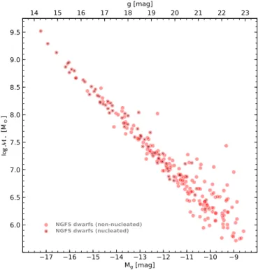
(12) The Astrophysical Journal, 855:142 (19pp), 2018 March 10. Eigenthaler et al.. (2005), Kirby et al.concluded that this relation is roughly continuous from the least massive systems at = 10 3.5 M to the most massive giant ellipticals at = 1012 M. Our most massive dwarf galaxy has log = 9.42, corresponding to a metallicity of [Fe/H];−0.66, if it follows the Kirby et al. (2013) relation.Considering standard abundances from Asplund et al. (2005), this converts to a metallicity of Z; 0.003.Hence, based on the BC03 (g′−i′)0 model tracks, one can expect ages of at least 5 Gyr for the average dwarf in our NGFS sample. While showing the expected low metallicities, we note that the dwarf candidate sample exhibits a large spread in metallicity if it is mostly uniformly old, that is,older than ∼10 Gyr.This might be explained by the host cluster environment that is likely to have experienced epochs of significant chemical inhomogeneities and, hence, may have uniquely influenced the star formation histories of the individual galaxies.However, the difficulty in breaking the age–metallicity degeneracy with u′g′i′ photometry alone is obvious.Future imaging campaigns that sample different regions of the spectral energy distribution (e.g., Muñoz et al. 2014) and deep integrated-field spectroscopy (e.g., Mentz et al. 2016) will be very valuable in further constraining the stellar population properties of these low-mass NGFS galaxies to higher accuracy.We, thus, defer a more detailed stellar population analysis and a discussion of the build-up of the faint galaxy population (Boselli & Gavazzi 2014), including nearinfrared photometry information, to future work.. Figure 7. The stellar mass–luminosity relation for our sample dwarf galaxies. Stellar masses are estimated using the prescription of Bell et al. (2003) utilizing the derived and dereddened (g′ − i′)0, (u′ − g′)0, and (u′ − i′)0 colors. Black dots denote nucleated dwarfs.. 5. Discussion. 4.3. Stellar Masses. 5.1. Scaling Relations. In order to study the physical scaling relations of the dwarf galaxy sample in relation with other stellar systems, we compute the stellar masses of our NGFS dwarf candidates using the prescriptions from Bell et al. (2003), which are good matches for the expected star formation histories of our NGFS spheroidal dwarf galaxies (Zhang et al. 2017). We parameterize the stellar mass-to-light ratios ( L ) by galaxy colors using the relation log ( L ) = al + bl ´ color,. Elliptical galaxies are known to fall on a so-called fundamental plane (FP), a tight correlation between effective radius, central velocity dispersion, and the average effective surface brightness within the effective radius (e.g., Faber & Jackson 1976; Djorgovski & Davis 1987; Dressler et al. 1987; Faber et al. 1987; Bender et al. 1992; Burstein et al. 1997; Gallazzi et al. 2006).A similar relation was found by Tollerud et al. (2011), showing that dispersion-supported galaxies form a one-dimensional fundamental curve in the mass–radius– luminosity space from ultrafaint dwarf spheroidals to giant cluster spheroids.Since the FP shows very little residual scatter, it implies very similar mass-to-light ratios and suggests a uniform formation process for bright elliptical galaxies. Projecting the FP onto the luminosity versussurface-brightness plane, Kormendy (1985) had noted that there seems to be a dichotomy between the scaling relations of bright elliptical galaxies and dwarf galaxies.This dichotomy can be interpreted as the result of different formation mechanisms for giant ellipticals and dwarf spheroids, but it is still hotly debated in the literature (e.g., Binggeli 1994; Graham & Guzmán 2003; Ferrarese et al. 2006; Kormendy et al. 2009; Kormendy & Bender 2012).In order to investigate these possible differences in the formation process of dwarf galaxies in comparison to bright elliptical and spiral galaxies, we plot in Figure 8 the effective radius (reff, in units of parsec) as a function of stellar mass M and in Figure 9 the effective mass surface 2 , in units of Me pc−2) as a density (Seff, = 2preff function of stellar mass M for our NGFS galaxy sample. We put the measurements in the larger context of several other families of stellar systems, covering a wide range in galaxy. (2). where the coefficients aλ and bλ define the transformation for different filter combinations, that is,colors (see Bell et al. 2003, their Table 7).We compute the g′- and i′-band L from our measured and dereddened (g′ − i′)0, (u′ − g′)0, and (u′ − i′)0 galaxy colors, yielding up to six estimates for a given galaxy.To compute , we derive galaxy luminosities in g′ and i′ considering absolute solar magnitudes measured by C. Willmer.22Finally, we average the individual estimates and adopt error bars as the standard deviation of the sample of individual measurements.We obtain stellar masses in the range 5.5 log M 9.4 .Figure 7 shows the comparison of the derived stellar masses with the apparent and absolute g′-band magnitudes.The corresponding values, in the following always given in units of Me, are summarized in Table 1.. 22. http://mips.as.arizona.edu/∼cnaw/sun.html. 12.
(13) The Astrophysical Journal, 855:142 (19pp), 2018 March 10. Eigenthaler et al.. Figure 8. Effective radius (reff in units of parsec) versus stellar mass ( in units of Me) parameter space for NGFS galaxies (red symbols) and various other stellar systems (see legend) with lines of iso-Seff, º M (2pre2 ) indicated.The top ordinate shows the corresponding absolute g′-band luminosity scaled by the average relation from Figure 7.The parameter space is split into extended and compact stellar systems at re=100 pc highlighted by the horizontal dotted line. We also show the average seeing limit of our observations measuring ∼1.4 arcsec. Curves of equal relaxation timescales for re - parameter combinations are indicated for various fractions of the Hubble time (thick dash-dotted curves).The Zone of Exclusion (thick dashed line) illustrates the stellar density limit beyond which virtually no objects are found.The line of maximum stellar surface density (Σmax ≈ 1011.5 Me kpc−2) observed for dense stellar systems in the nearby universe is also indicated (see Hopkins et al. 2010).Similar relations for the ATLAS3D data sets from Cappellari (2016) are plotted for two dynamical to stellar mass ratios, dyn = 1 and 5.The brown curve indicates a LOWESS fit to the NGFS dwarfs and other early-type galaxy data from the literature, while the blue curve is a LOWESS fit to the NGFS dwarfs and massive spiral galaxies only.The inset plot in the bottom right corner shows the gradients of these curves with three stellar mass zones dominated by different galaxy mass accumulation processes (see the text for details).. systems further in this work, noting only that numerous recent studies have described the formation scenario of UCDs via tidal stripping of galaxies with NSCs on relatively short timescales (e.g., Bekki et al. 2003; Goerdt et al. 2008; Thomas et al. 2008; Pfeffer & Baumgardt 2013; Pfeffer et al. 2014, 2016; Liu et al. 2015; Zhang et al. 2015).Instead, we focus in the following on the extended stellar systems and the larger galaxy evolution context of our NGFS galaxy sample. The NGFS sample dwarfs cover stellar masses in the range log » 5.5–9.5 (see also Figure 7).The bulk of the NGFS dwarfs show Seff, values in the range ∼1–10 Me pc−2, with the most massive dwarfs reaching ∼100 Me pc−2 (see Figures 8 and 9).Dwarf galaxies with relatively low stellar masses (log 5.5–8.0 ) follow a scaling relation with reff. morphology and stellar mass from low-mass LG dSph galaxies with log » 3 to giant elliptical galaxies at log » 12. For the subsequent discussion, we divide the reff– and Seff, – diagrams in two hemispheres with (1) extended stellar systems (log reff [pc] 2.0 ), such as dwarf spheroidal galaxies, dE, and giant elliptical (gE) galaxies, and (2) compact stellar systems (log reff [pc] 2.0 ) with two subsets, one of which represents globular clusters with two-body relaxation times shorter than a Hubble time (i.e., objects below the curve trelax = Hubble time) and the other subset comprising nonrelaxed compact stellar systems, such as nuclear star clusters (NSCs) and ultracompact dwarfs (UCDs).For a description of this part of the parameter space, we refer the reader to Misgeld & Hilker (2011).We will not discuss the compact stellar 13.
(14) The Astrophysical Journal, 855:142 (19pp), 2018 March 10. Eigenthaler et al.. Figure 9. Effective surface mass density (Seff, ) versusstellar mass ( ) parameter space for NGFS galaxies (red symbols) and various other stellar systems (see legend). Solid diagonal lines mark constant effective radius, i.e.,iso-reff lines. Other curves and lines correspond to those in Figure 8.The top ordinate shows the corresponding absolute g′-band luminosity scaled by the average relation from Figure 7, while the right abscissa gives the effective surface mass density in units of Me pc−2.. log » 5.5–12.0: (A) NGFS dwarfs + Virgo ETGs (Ferrarese et al. 2006) + Carnegie-Irvine E galaxies (Ho et al. 2011) shown as a brown curve; and (B) NGFS dwarfs + spiral galaxies from the ATLAS3D survey23 (Cappellari et al. 2011) illustrated as a blue curve.While sample A assumes that dwarf galaxies are evolutionarily connected to more massive early-type galaxies through their morphology, sample B joins, somewhat ad hoc, the dwarf galaxy regime with more massive spirals under the premise that they form a dynamical family in which the angular momentum increases with stellar mass (for a discussion, see Cappellari 2016). We disregard the class of UDGs for the rest of this work (but see Amorisco & Loeb 2016; Rong et al. 2017, for a theoretical discussion of this galaxy type), but note that the scaling relations in Figures 8 and 9 show a few NGFS objects consistent with massive dwarf galaxy candidates (7.5 log M 8.5). that is positively inclined with respect to the lines of equal effective surface mass density, oriso-Seff, lines (see diagonal lines in Figure 8).Meanwhile, recent studies have revealed an expansive population of low-mass dwarfs in the Local Group, including dSphs and UFDs that extend toward even fainter magnitudes (Zucker et al. 2004, 2006a, 2006b; Willman et al. 2005; Belokurov et al. 2006, 2007, 2010, 2014; McConnachie et al. 2009; McConnachie 2012; Bechtol et al. 2015; Drlica-Wagner et al. 2015; Koposov et al. 2015; Laevens et al. 2015; Homma et al. 2016).Their size–mass–surface density scaling relations appear to line up seamlessly with our NGFS dwarf sample toward lower stellar masses and lower surface mass densities. We approximate the scaling relations of our NGFS dwarfs with a locally weighted scatterplot smoothing (LOWESS) fit (e.g., Cleveland 1981), which is illustrated as a thick curve in Figures 8 and 9.To connect the LOWESS fit of the NGFS dwarf sample with more massive galaxies, we construct two samples that span the full stellar mass range. 23. We point out that we do not include the early-type ATLAS3D galaxies in sample A due to their relatively shallow stellar mass limit (∼109.5 Me).. 14.
(15) The Astrophysical Journal, 855:142 (19pp), 2018 March 10. Eigenthaler et al.. beginning to encroach upon the parameter space occupied by UDGs, the existence of which has been recently reported in massive galaxy groups and clusters (e.g., Koda et al. 2015; Mihos et al. 2015; Muñoz et al. 2015; van Dokkum et al. 2015a; Martínez-Delgado et al. 2016; Merritt et al. 2016; Bennet et al. 2017; Janssens et al. 2017; Román & Trujillo 2017b; Shi et al. 2017; Trujillo et al. 2017; van der Burg et al. 2017; Venhola et al. 2017).UDGs show physical sizes reminiscent of giant galaxies, but values that put them in the dwarf galaxy mass regime.The result is a systematically lower Seff, that detaches UDGs from the scaling relations shown by the other dwarfs and intermediate stellar mass galaxies.Given their existence and characteristics, one might speculate that these galaxies are dominated by dark matter, shielding the baryons from the cluster environment (e.g., Mihos et al. 2015; Mowla et al. 2017).. hierarchical galaxy formation picture has been extensively discussed in the recent literature (for a recent review, see Cappellari 2016, and references therein). Based on the present NGFS data and the comparison with other stellar systems from the literature, the following discussion aims to highlight the implications of our findings for galaxy mass assembly over a stellar mass range of 5 log 12. We want to emphasize that this discussion does not necessarily imply an evolutionary sequence in the sense that more massive stellar systems arise from less massive ones observed today. It is merely an empirical observation based on the derived gradients from Section 5.2 on how mass assembly occurs in these galaxies at various stellar masses. First, we note that mass assembly along the iso-Seff, lines implies virtually density-invariant growth, indicating that to first order, mass assembly occurs homologously along these lines; as galaxies grow in size and stellar mass, they retain their surface brightness distribution and, hence, the effective stellar mass surface density. From Figure 8 we find that as early-type systems (sample A) grow in stellar mass, the assembly of baryonic mass must occur in various phases and under the influence of different mechanisms, which depend on the total stellar mass of the system, for the observed relations to emerge. For dwarf galaxies, this mass assembly process occurs biased to regions inside the half-light/mass radius since the systems grow disproportionately more dense within reff as stellar mass increases; that is,their reff– relation is flatter with respect to the iso-Seff, lines.This trend prevails until approaches log » 8.0 , where the reff– relation becomes flat with significant scatter. The constancy of reff in this respective mass range had already been pointed out by Smith Castelli et al. (2008) and Misgeld et al. (2008) and implies that stellar mass is being added both inside and outside the galaxy half-light/stellar-mass radii so that galaxy stellar mass growth occurs without experiencing changes in galaxy sizes, that is, is isometric. Consequently, this mode of stellarmass growth is accompanied by packing increasingly more stellar mass within the same galaxy dimensions.This process may be triggered by ram pressure in dense galaxy cluster environments, which may temporarily induce enhanced star formation efficiency (e.g., Geha et al. 2012; Wetzel et al. 2013).The isometric stellar mass growth stops when the galaxies reach an apparent maximum stellar mass density of Seff, » 10 4 M pc-2 at around log » 10.5.Beyond this point toward higher values, galaxy stellar mass accumulation happens predominantly outside their half-light/mass radii, which is consistent with their reff– relations being steeper than the iso-Seff, lines.Similar findings have been put forward by studies of the redshift evolution of the reff– relation of massive galaxies (e.g., Huertas-Company et al. 2013; van Dokkum et al. 2015b). This observed transition from centrally dominated to halodominated stellar mass accumulation goes hand in hand with the transition from cusp to core-dominated central surface brightness profiles of galaxies more massive than log » 9.0 revealed by HST-based studies (see, e.g., Ferrarese et al. 2006; Côté et al. 2007).The homogeneous morphological analysis of our NGFS galaxy data set, with a much broader stellar mass coverage down to log » 5.5, shows the consistency of this central morphological transition with global Sérsic model parameters.While single-component Sérsic fits. 5.2. Scaling Relation Gradients For sample A, we find a galaxy size–mass scaling relation of 0.1 in the stellar mass range 5.5 the form reff µ 0.3 log 7.8, the gradient of which decreases abruptly to zero at log » 8.0 (i.e., LOWESS = D log reff D log » 0; see inset plot in Figure 8).The effective radius remains virtually independent of stellar mass for more massive galaxies and remains roughly constant at ∼1 kpc (albeit with a substantial scatter) up to about log » 9.5, where it begins to gently increase again until it jumps abruptly at log » 10.5 to values that are steeper than the iso-Seff, lines.The gradient at high stellar masses (log 10.8) 0.05 reaches reff µ 0.75 .For sample B, the gradient of the size–mass relation is relatively constant over the entire 0.1 . mass range (log » 5.5–12) around reff µ 0.25 Although we are dealing with incomplete and partly nonoverlapping parameter ranges for the individual data sets depicted in Figures 8 and 9, we observe a smooth transition between the low-mass dwarf regime over the range of intermediate stellar mass systems to the massive galaxies for our self-consistently observed and analyzed sample of NGFS galaxies. Here, the scaling relations become particularly diagnostic in the intermediate-mass regime (8.5 log 10.0 ), where the association of at least some of the NGFS galaxies with the sample B dynamical family cannot be excluded. Testing the internal dynamics of such galaxies is, therefore, of utmost interest. The literature samples are augmenting the information content of the scaling relations for our NGFS data by extending its parameter space coverage, which leads us to the following discussion and interpretation of our measurements. 5.3. Implications for Galaxy Mass Assembly Dwarf galaxies in cluster environments are believed to have been and some are presently being affected by their environment, which is one of the mechanisms for the creation of the morphology–density or morphology–distance relation for dwarfs.Environmental effects include tidal stripping, ram pressure stripping, and harassment. Moreover, internal effects may play a role. For instance, winds have been invoked as one of the factors affecting their chemical enrichment, and feedback, in general, may have led to mass loss.How the size–stellar mass (i.e., reff– ) scaling relation for extended stellar systems can be interpreted in the context of the 15.
Figure


+4


Documento similar
