Evaluation of Feature Extraction Techniques for an Internet of Things Electroencephalogram

(1)

Electronics Engineering School

Karslruhe Institute of Technology Chair for Embedded Systems

Evaluation of Feature Extraction Techniques for

an Internet of Things Electroencephalogram

Thesis in fulfillment of the requirements to obtain the academic degree of Licentiate in Electronics Engineering

David Barahona Pereira

(2)

(3)

(4)

(5)

(6)

(7)

Abstract

The emerging paradigm of Internet of Things (IoT) is revolutionizing our life with the introduction of new services and the improvement of existing applications. IoT is covering an ever-increasing number of applications in different domains including healthcare. One specific application in personal healthcare is the monitoring of the electrical activity in the brain using Electroencephalogram (EEG) with portable IoT devices. Due to portability and size constraints, most IoT devices are battery-powered which calls for energy-efficient implementation in both hardware and software along with an efficient use of the often limited resources.

This work evaluates three different feature extraction techniques for an IoT EEG in terms of execution time, memory usage and power consumption. The techniques under study were explored and simulated leading to select FIR, Welch’s method and DWT as the ones to be evaluated. The techniques were implemented on a MSP432P401R LaunchPad platform, where an evaluation procedure was developed to asses the code performance. The implementations were validated against simulated references and also optimized for speed, code size and power consumption. The result of the performed evaluation provides a valuable comparison between the techniques which can help any designer in choosing the right technique based on design objectives and resource constraints.

(8)

(9)

(10)

(11)

Acknowledgments

First, I would like to thank my thesis advisor Farzad Samie at the Karlsruhe Institute of Technology (KIT) for letting me be part of his research and for being always attentive and supportive during the development of the project. Also, I would like to thank my thesis advisor Renato R´ımolo at the Costa Rica Institute of Technology (ITCR) for all his recommendations and for always being pending of my progress despite the distance. I would like to thank all the people that in one way or another made possible for me to develop my project not only in Germany but also in such a remarkable institution as the KIT. I want to thank my friend Moises Araya and my teacher Jorge Castro for helping me find a project but specially for all their support, trust and recommendations. Also, I would like to thank the ITCR for promoting this kind of experiences and specially to Gustavo Rojas from the Construction Engineering School for all his help.

Thanks to all my friends who have accompanied me until this point, specially to Esteban and Adolfo who more than friends have become brothers to me. After all these years of working together I can be pretty sure that we make a great team together, thank you for all those endless nights of study and projects but specially for always being there.

Last but not least, I must express my very profound gratitude to my family. I want to thank them for providing me with unconditional love, unfailing support and continuous encouragement throughout all my life and years of study. Thank you for being always my everyday motivation. I would especially like to thank my mother for all her love and dedication throughout all these years. Thank you for being my best friend and the person I admire the most, there are no words that can describe how much I love you and how thankful I feel. This accomplishment would not have been possible without you.

(12)

(13)

List of Figures

1.1 Stages of the project . . . 2

2.1 EEG device . . . 6

2.2 EEG frequency bands . . . 6

2.3 EEG signal processing path . . . 7

2.4 Welch’s method procedure . . . 12

2.5 Single level DWT . . . 13

2.6 Multilevel DWT . . . 13

2.7 WPT decomposition . . . 14

3.1 EEG test signal . . . 17

3.2 FIR filter response for the Alpha band . . . 18

3.3 Power for the Alpha band using FIR filter . . . 19

3.4 IIR filter response for the Alpha band . . . 19

3.5 Power for the Alpha band using IIR filter . . . 20

3.6 Comparison of FIR and IIR . . . 20

3.7 Periodogram on the EEG signal . . . 22

3.8 Welch’s method on the EEG signal . . . 22

3.9 Comparison of periodogram and Welch’s method . . . 23

3.10 Low-pass decomposition filter response for DWT . . . 24

3.11 High-pass decomposition filter response for DWT . . . 24

3.12 DWT decomposition of the EEG signal . . . 25

3.13 WPT decomposition of the EEG signal . . . 26

3.14 Comparison of DWT and WPT . . . 27

3.15 Comparison of filter and DWT based techniques . . . 28

3.16 Comparison of filter, FFT and DWT based techniques . . . 28

4.1 CCS Breakpoints tab . . . 32

4.2 CCS Memory Allocation tab . . . 34

4.3 Profile tab in ET mode . . . 35

4.4 Power tab in ET mode . . . 36

4.5 Energy tab in ET mode . . . 36

4.6 Profile tab in ET+ mode . . . 37

4.7 States tab in ET+ mode . . . 37

(16)

iv List of Figures

5.1 FIR feature extraction algorithm sequence . . . 41

5.2 Simulated and microcontroller comparison for FIR . . . 42

5.3 Validation error for FIR . . . 42

5.4 Welch’s method feature extraction algorithm sequence . . . 43

5.5 Rectangular window . . . 44

5.6 Simulated and microcontroller comparison for Welch’s method . . . 45

5.7 Validation error for Welch’s method . . . 45

5.8 DWT method feature extraction algorithm sequence . . . 46

5.9 Bookkeeping vector structure for DWT . . . 47

5.10 Rearrangement of coefficients process for DWT . . . 48

5.11 Simulated and microcontroller comparison for DWT . . . 48

5.12 Implemented bookkeeping vector for DWT . . . 49

5.13 Validation error for DWT . . . 49

5.14 Compiler optimization view . . . 50

5.15 Code size for different optimization level settings . . . 51

5.16 Code size for different code size and speed trade-off settings . . . 51

5.17 Power measurements for optimization . . . 53

5.18 Energy measurements for optimization . . . 54

6.1 Execution time evaluation . . . 56

6.2 Flash memory usage evaluation . . . 57

6.3 SRAM memory usage evaluation . . . 57

6.4 Power consumption evaluation . . . 59

(17)

List of Tables

2.1 Cognitive states related to EEG frequency bands . . . 7

2.2 Feature extraction techniques comparison . . . 16

3.1 Bands obtained using DWT . . . 25

3.2 Bands obtained using WPT . . . 26

5.1 Validation percentage error for FIR . . . 43

5.2 Validation percentage error for Welch’s method . . . 45

5.3 Validation percentage error for DWT . . . 49

5.4 Compiler optimization settings . . . 51

5.5 Speed optimization . . . 52

5.6 Code size optimization . . . 52

5.7 Power measurements for optimization . . . 53

5.8 Energy measurements for optimization . . . 54

6.1 Execution time evaluation . . . 55

6.2 Memory usage evaluation . . . 57

6.3 Power consumption evaluation . . . 58

6.4 Overall evaluation of feature extraction techniques . . . 60

(18)

(19)

Chapter 1 Introduction

The Internet of Things for Healthcare group of the Chair for Embedded Systems (CES) at the Karlsruhe Institute of Technology (KIT) is devoted to the research of solutions and novel techniques to address challenges in Internet of Things (IoT) and particularly, wearable healthcare monitoring systems. Wearable healthcare monitoring systems can be used to monitor patients who are out of the hospital, they can measure daily or sport activities, and they can even keep track of sleep patterns and stress levels. Part of the current research activities at Internet of Things for Healthcare group is the development of a wearable IoT Electroencephalogram (EEG) prototype.

An EEG is a device that is able to measure and record the electrical activity of the brain. EEG is commonly found in medical applications, however its use has been extended to other fields such as Brain Computer Interfaces (BCIs) in tasks like controlling a robotic arm by imagining hand movements [27]. An IoT EEG is intended to be a portable and hence battery-powered device, therefore it is important to find the best way to face inherent challenges in computation capability and energy capacity. One of the stages in the operation of an EEG is feature extraction, this stage uses several signal processing techniques to get relevant information about the brain activity usually by measuring power in different frequency bands. Since there are many techniques that can be used in feature extraction, it is important to compare them in order to develop a criteria about which can be better suited to face the previously mentioned challenges.

This work evaluates different feature extraction techniques from perspectives such as execution time, memory usage and power consumption in a microcontroller platform. In order to achieve that goal, the process depicted in Figure 1.1 can be followed. There are mainly three different approaches that can be used for feature extraction such as filtering, Fast Fourier Transform (FFT) and Discrete Wavelet Transform (DWT). However, there are plenty of feature extraction techniques that use one or even combinations of those approaches. Therefore, the first stage of the solution involves an extensive investigation about which are the most relevant techniques that use either filters, FFT or DWT for feature extraction, as well as their characteristics and possible optimization schemes.

(20)

2

The simulation stage uses the findings of the previous investigation to explore how each of the techniques under study behaves in the presence of a real EEG signal. The goal is to consider the characteristics of each technique and the results from the simulations to select three techniques for implementation, one using filters, one using FFT and one using DWT. A comparison between techniques is performed in order to make sure that they all provide similar information and therefore work correctly. The simulation results will also work as a reference to validate the implementations.

The selected platform for the implementation is a MSP432P401R LaunchPad from Texas Instruments which incorporates a microcontroller designed for low-power applications. In the platform setup stage, the goal is to find a procedure to measure the parameters that will be evaluated. A procedure to measure execution time, power consumption and memory usage is developed in this stage.

The implementation stage is the core of the solution and it consists in implementing each selected technique in the microcontrolller platform. Here, the correct behavior of each technique needs to be validated and also since the main approach is to face computation and power challenges, possible optimizations must be carried out as well.

In the final stage, execution time, power consumption and memory usage are measured using the procedure developed in the setup stage. The results are documented and serve to compare each technique in order to evaluate how they fit in the final design of the device.

Investigation

Simulation

Platform setup

Implementation

Evaluation

(21)

1.1 Document Structure

This document is organized as follows:

Chapter 2 reviews EEG fundamentals, the commonly used signal processing path and delves into feature extraction techniques. Theoretical background for filters, FFT and DWT is provided and also techniques that use those approaches are explained emphasizing the most relevant characteristics, advantages and disadvantages.

Chapter 3 provides simulations for the techniques under study in order to show how they perform in the presence of a real EEG signal. It also takes those results and the ones of the investigation stage to decide which techniques are chosen for implementation.

Chapter 4 provides a brief introduction of the low-power microcontroller platform under use and its characteristics. It also states the procedure to follow for measuring execution time, power consumption and memory usage.

Chapter 5 shows the approach taken for each implementation along with results that validate that they behave as intended. Optimizations carried out for each of the metrics under test are also explained in this chapter.

Chapter 6 provides the results of the measurements for each technique and makes an analysis to evaluate the implementations and form a criteria about how each technique fits in the design of an IoT EEG.

(22)

(23)

Chapter 2 Feature Extraction Techniques in EEG

In order to understand feature extraction techniques it is important to set a background of what is an EEG and how it works. This chapter provides some basic notions of what is an EEG and which is the signal processing path commonly used to deal with brain activity measurements. It provides not only a theoretical background for filters, FFT and DWT approaches but also discusses the most common techniques that makes use of those approaches. Finally, it makes a comparison of the techniques by exploring characteristics, advantages and disadvantages.

2.1 EEG and Applications

Human body imaging techniques play a crucial role in modern medicine. Electrobiological measurements can be divided as electrocardiography (ECG), electromyography (EMG), electroencephalography (EEG), magnetoencephalography (MEG), electrogastrography (EGG) and electrooculography (EOG).

An EEG is a test device used to evaluate the electrical activity in the brain. Since brain cells communicate with each other through electrical impulses, EEG can be used to detect potential problems associated with this activity. The test is typically noninvasive, it tracks and records brain wave patterns through a set of electrodes attached to the scalp with wires as depicted in Figure 2.1.

Measurements given by an EEG can be used to rule out various conditions, including seizure disorders (such as epilepsy), a head injury, encephalitis (an inflammation of the brain), a brain tumor, encephalopathy (a disease that causes brain dysfunction), memory problems, sleep disorders, stroke, dementia and many others. The use of this device has been extended to other fields such as social interaction [4], marketing [5], psychology [28] or BCIs [27] [33].

(24)

6 2.1 EEG and Applications

Figure 2.1: EEG device. Source: www.saintlukeshealthsystem.org

Measurements taken from an EEG consist of an electrical wave that varies in time, much like a sound signal or a vibration. As such, it contains frequency components that can be measured and then analyzed, these frequency components have interesting and valuable properties. As shown in Figure 2.2, brain waves have been categorized according with their frequency range into four basic groups known as: Delta, Theta, Alpha and Beta.

0 100 200 300 400 500

(25)

Most applications generally focus on the spectral content of EEG, that is, the type of neural oscillations that can be observed in EEG signals [7]. Table2.1shows the frequency range of each brain wave and also the specific brain activity associated with each band.

Table 2.1: Cognitive states related to EEG frequency bands Band Frequency range (Hz) Brain activity

Delta 0.5-4 Deepest meditation and dreamless sleep

Theta 4-8 Light sleep

Alpha 8-13 Relaxation

Beta +13 Consciousness

2.2 Signal Processing Path

Most modern applications follow a common path for EEG signal processing as depicted in Figure 2.3. Raw EEG signals go to a preprocessing stage mostly to deal with artifacts and noise. Then, relevant features about the brain activity are extracted and finally those features are classified to determine a mental state.

Preprocessing Raw EEG

Feature extraction

Classification

Output

(26)

8 2.3 Feature Extraction Techniques

2.2.1 Preprocessing

The preprocessing stage can include the acquisition of the signal, removal of artifacts, averaging, thresholding of the output, enhancement of the resulting signal, and finally, edge detection. The most critical step in this stage and in many others signal processing applications is the removal of artifacts. There are many sources of artifacts in recording raw EEG signals [15]. They can be defined as disturbances that may occur during the signal acquisition and that can alter the analysis of signals themselves. Useful features of the original signal can be severely affected if noise is not properly treated. Some sources of artifacts can be muscular activities, blinking of eyes during the signal acquisition procedure and power line electrical noise.

2.2.2 Feature Extraction

It is difficult to extract useful information from EEG signals just by observing them in the time domain. Therefore, there are many advanced signal processing techniques that can be used to extract relevant features from those signals [6] [12]. The choice of a particular technique is usually tied to the application under study and specific requirements. Feature extraction aims at describing relevant information about the brain activity by an ideally small number of relevant values. All extracted features are usually arranged into a vector, known as a feature vector, which is used later for the brain activity classification. There are three main sources of information that can be extracted from EEG readings: spatial information (for multichannel EEG), spectral information (power in frequency bands) and temporal information (time windows based analysis) [9].

2.2.3 Classification

The last stage is denoted as classification and it consists of assigning a class to a feature vector corresponding to the mental state. Just as for the feature extraction stage, there are many classification methods that may suit a specific implementation better than others. In [31], a comparison of performance for different classification methods for EEG based BCIs is proposed.

2.3 Feature Extraction Techniques

(27)

2.3.1 Filter Based Feature Extraction

Filters are devices that allow some signal frequencies applied at their input terminals to pass through to their output terminals with little or no reduction in the signal level. There are analog and digital implementations of filters and the use of one or another will depend of the nature of the signals in the system whether there are continuous or digital signals. Digital filters are systems commonly used in signal processing to deal with discrete time signals. They often consist of an analog to digital converter, a processing stage and a digital to analog converter.

One popular way to compute band power features from an EEG signal is to use band-pass filters to extract each desired band to later estimate energy. The process to follow is to first take an interval of the signal, e.g. 250 ms [23], then band-pass the EEG signal to each band of interest, square each sample and finally average the signal over several consecutive samples. This approach is commonly found in BCI research, e.g. in OpenViBE software [26] this is the method performed by default.

There are two types of digital filters, each with advantages and disadvantages: the Finite Impulse Response (FIR) filters and the Infinite Impulse Response (IIR) filters [32]. FIR filters have no feedback so their impulse response is of finite duration because it settles to 0 after some time. For an FIR filter of order N, the output sequence consists of a weighted sum of past input values:

y[n] =

(28)

In contrast to FIR filters, IIR filters have feedback and their impulse response does not become exactly 0 past a certain point, but continues indefinitely. The output depends not only of past input values but also from past output values:

y[n] = N

X

i=0

bix[n−i] + M

X

j=0

ajy[n−j] (2.2)

where:

y[n] = output signal

x[n] = input signal

N = feedforward filter order

M = feedback filter order

bi = feedforward filter coefficients

ai = feedback filter coefficients

IIR filters are more complex and are well suited in applications where a sharp fall-off or phase is not critical but when flat pass-bands and stop-bands are important. They exhibit a smaller delay than FIR and use less elements to calculate the output. However, they show a non-linear phase response and can become unstable. For both types of filters, the desired response is given by the set of coefficients that multiply each past input or output.

2.3.2 FFT Based Feature Extraction

(29)

The DFT is defined by the formula:

N = elements in input sequence

FFT is commonly used in EEG to estimate Power Spectral Density (PSD). PSD refers to the spectral energy distribution that would be found per unit frequency. It can be computed by applying FFT directly on the signal or also by transforming the estimated autocorrelation sequence. In [20] a comparison of PSD estimation methods for EEG is shown. Among the techniques that use FFT for feature extraction, the periodogram and Welch’s method are two of the most popular and commonly exploited.

The easiest approach to compute PSD is the periodogram. It consists of a frequency decomposition and is given by the modulus squared of the Fourier transform of the signal:

S(f) = ∆t

∆t= space between samples

xn = input sequence

N = elements in input sequence

(30)

On the other hand, Welch’s method is an improvement on the standard periodogram [10]. It is based on the use of overlapping windows to the signal in which a periodogram is calculated for each window and then those periodograms are averaged between them to compute PSD. This procedure is depicted in Figure 2.4. This method reduces variance and hence noise in the estimated power spectra in exchange for reducing the frequency resolution [1].

Periodogram Periodogram Periodogram Periodogram Averaging

Time (s) Voltage (V)

Figure 2.4: Welch’s method procedure

2.3.3 DWT Based Feature Extraction

(31)

DWT is a decomposition that uses discrete sampled wavelets and is usually implemented using filters. Figure 2.5 shows a single level DWT implementation. The signal goes through a high-pass filter and a low-pass filter that are related as quadrature mirror filters. The high-pass filter provides details coefficients and the low-pass filter provides approximation coefficients. After filtering, since half of the frequencies have been removed, a subsampling is applied to reduce the amount of data because only half of the samples are needed to represent the new signal according to Nyquist’s sampling theorem [22].

h[n]

Figure 2.5: Single level DWT decomposition of a signal

There are also multilevel approaches that aim a better frequency resolution as depicted in Figure 2.6. In these implementations another DWT is applied to the approximation coefficients [34].

Figure 2.6: A multilevel DWT decomposition of a signal

(32)

Wavelets have some slight benefits over Fourier transforms in reducing computations when examining specific frequencies. This method uses varying window sizes so it does not suffer the time-frequency resolution trade-off inherent to other time-frequency approaches [35]. WPT is a variation of the classic DWT that uses more filters in the implementation. The difference with the simple DWT is that this approach computes a DWT not only in the approximation coefficients but also in the details coefficients for each level, building a binary tree. A WPT decomposition is shown in Figure 2.7.

g[n] 2

Figure 2.7: A multilevel WPT decomposition of a signal

(33)

2.3.4 Feature Extraction Techniques Overview

The performed analysis can lead to have a better picture of how filters, FFT and DWT can be used as feature extraction techniques and how they possess certain characteristics that can be exploited depending on a specific application.

Filtering analysis is performed in the time domain and may not be the best to deal with non-stationary signals. The performance of a filter is tied its order and the type of filter. FIR filters are fairly simple, always stable and show a linear phase response, however they have a delay that could be critical in certain applications and also they are not very efficient since they use a lot of inputs to calculate the output. On the other side, IIR filters are more efficient since they use less inputs to calculate the output and therefore they have only a small delay, however they are more complex, they can become unstable and they modify the output because of the non-linearity of the phase response.

FFT analysis is performed in the frequency domain and just like filtering is not well suited for non-stationary signals. The periodogram is a low complex mechanism of computing PSD with a good frequency resolution, however it comes to a cost of producing spurious artifacts that could add a lot of noise to the signal. Welch’s method is a variation of the periodogram that manages to reduce noise in the computation while sacrificing frequency resolution.

Finally, DWT is a technique that performs in both time and frequency domain and is well suited for non-stationary signals. There must be a careful selection of the mother wavelet function and decomposition level. DWT is less complex and has less frequency resolution than the WPT that can achieve a better decomposition and therefore a better resolution by using more filters but adding complexity to the design.

(34)

Table 2.2: Feature extraction techniques comparison

(35)

Chapter 3 Simulation and Exploration of Feature

Extraction Techniques

In this chapter a set of MATLAB [16] simulations are presented in order to explore the behavior of the techniques studied in Chapter 2. For each technique two approaches were individually tested and then compared to select one to be implemented and evaluated in a microcontroller. Even though each technique provides information about the bands in different manners, they are compared in order to verify that they all provide similar and correct information. Lastly, the results of the simulations will be used to later validate the implementations. Every power or power density measurement for the frequency bands is normalized to a 1 Ω resistor for simplicity.

3.1 Test Signal

The signal in Figure 3.1 was selected in order get more representative simulations.

0 50 100 150 200 250 300 350 400 450 500 −150

−100 −50 0 50 100 150

EEG Signal

Sample

Voltage (uV)

Figure 3.1: EEG test signal

(36)

18 3.2 Filter Based Techniques

The signal was taken from a dataset created and contributed to PhysioNet [11] by the developers of the BCI2000 [29] [30] instrumentation system that was used to make these recordings. The experimental procedure for the measurements can be consulted in [24]. The selected input signal was sampled at 160 Hz, with 512 samples and hence a duration of 3.2 s.

3.2 Filter Based Techniques

FIR and IIR approaches are individually simulated and then compared. The procedure to use filters as feature extraction technique is to pass the EEG signal through a set of band-pass filters to later compute power and finally to average it over time to reduce noise. The result is a time domain representation of power for each band.

Each filter must be designed separately since all of them have different cut-off frequencies depending on the band of interest. The order of the filter must be selected in order to get a good trade-off between complexity and performance. The criteria to design the filters was the get the lowest order that ensured an attenuation equal or less than 3 dB in the pass-band. Power was computed just by squaring the voltage reading and a moving average filter was applied to the power signal in order to reduce noise.

3.2.1 FIR

The designed FIR filter is of order 60, so it has 61 taps. The magnitude and phase response for the filter designed for the Alpha band can be observed in Figure 3.2, the same approach was taken with the other bands.

0 0.1 0.2 0.3 0.4 0.5 0.6 0.7 0.8 0.9 1

−1000 −500 0 500

Normalized Frequency (×π rad/sample)

Phase (degrees)

Magnitude (dB)

(37)

After passing the input signal through the filter, power is computed and averaged over time to get the power reading shown in Figure 3.3

0 50 100 150 200 250 300 350 400 450

Figure 3.3: Power for the Alpha band using FIR filter

3.2.2 IIR

The same design approach was used for IIR filters. In this case, the filter is of order 3 with a Butterworth response that is intended to have a frequency response as flat as possible in the pass-band. The magnitude and phase response of the filter is shown in Figure 3.4

0 0.1 0.2 0.3 0.4 0.5 0.6 0.7 0.8 0.9 1

Phase (degrees)

Magnitude (dB)

(38)

20 3.2 Filter Based Techniques

The power signal for the Alpha band is depicted in Figure 3.5

0 50 100 150 200 250 300 350 400 450

0 100 200 300 400 500 600 700

Alpha Band Power (8 Hz − 13 Hz)

Sample

Power (pW)

Figure 3.5: Power for the Alpha band using IIR filter

3.2.3 Comparison

A comparison of the two filters is presented. Figure 3.6 shows power for FIR and IIR filters working in the Alpha band.

0 50 100 150 200 250 300 350 400 450

0 100 200 300 400 500 600 700

Alpha Band Power (8 Hz − 13 Hz)

Sample

Power (pW)

FIR IIR

(39)

The power plot shows that the shape of both curves is almost identical with slightly differences. There is a small difference in amplitude that is associated to a small variation between the gain of the filters in the pass-band, the magnitude response of the IIR filter is not as sharp as the FIR counterpart so it means there is more gain in certain frequencies. There are also small differences in shape due to the linearity of the phase response, however those differences are not critical. Finally, there is a small time shift as expected since IIR has a smaller delay than FIR. Since both approaches showed similar results and the observed differences are not critical for the application, FIR is the algorithm to be implemented since it is able to get satisfactory results with much less complexity in implementation than IIR.

3.3 FFT Based Techniques

Periodogram and Welch’s method are also simulated and compared as feature extraction techniques. Both approaches aim to compute PSD for different frequencies. The result is a frequency domain representation of power in which each frequency band is contained in a finite amount of samples depending on the frequency resolution. Frequency resolution will depend of the number of points used to compute the FFT to the whole signal or to a time window in the signal. Power after the FFT is normalized so the units of the PSD are W/Hz, however it is usually represented in dB/Hz by taking the base 10 logarithm of the power.

3.3.1 Periodogram

A simple periodogram can be applied to the EEG signal in order to compute PSD. In this case the periodogram definition given in equation2.4 was applied to the input signal, using a 512 points FFT. Therefore, for this approach the output has 256 samples with a frequency resolution of 0.3125 Hz/sample. The results of the simulation can be observed in Figure 3.7.

3.3.2 Welch’s Method

(40)

22 3.3 FFT Based Techniques

0 50 100 150 200 250

−160 −150 −140 −130 −120 −110 −100 −90 −80

Power Spectral Density

Sample

Magnitude (dB/Hz)

Figure 3.7: Periodogram on the EEG signal

0 10 20 30 40 50 60

−135 −130 −125 −120 −115 −110 −105 −100 −95 −90

Power Spectral Density

Sample

Magnitude (dB/Hz)

(41)

3.3.3 Comparison

A comparison of the periodogram and Welch’s method is depicted in Figure 3.9.

0 50 100 150 200 250

Figure 3.9: Comparison of periodogram and Welch’s method

Both plots depict a similar shape with some differences. As expected, the periodogram provides a good frequency resolution in trade of a noisy reading. On the other hand, Welch’s method frequency resolution is smaller but the plot has reduced variance and the power is not as noisy as the one from the periodogram. The noise present in the periodogram reading can provide erroneous information about the brain activity, Welch’s method is able to provide more accurate readings and can also supply information about each band using less points. Frequency resolution can be adjusted only by changing the window size and since it is not very complex when compared to the periodogram as it only includes some extra windowing and averaging, it is the selected method to be implemented.

3.4 DWT Based Techniques

(42)

24 3.4 DWT Based Techniques

0 0.1 0.2 0.3 0.4 0.5 0.6 0.7 0.8 0.9 1

−1000 −500 0

Phase (degrees)

0 0.1 0.2 0.3 0.4 0.5 0.6 0.7 0.8 0.9 1

−300 −200 −100 0 100

Magnitude (dB)

Figure 3.10: Low-pass decomposition filter response for DWT

0 0.1 0.2 0.3 0.4 0.5 0.6 0.7 0.8 0.9 1

−200 −100 0 100 200

Phase (degrees)

0 0.1 0.2 0.3 0.4 0.5 0.6 0.7 0.8 0.9 1

−300 −200 −100 0 100

Magnitude (dB)

(43)

3.4.1 DWT

In order to use DWT, a decomposition level must be selected depending on the sampling frequency. Since the signal is sampled at 160 Hz the decomposition level suited to extract the desired bands is 4. Table 3.1 shows which frequency bands can be obtained in each level and the amount of samples that relate to each band.

Table 3.1: Bands obtained using DWT Level Frequency (Hz) Samples Related band

4 0-5 38 Delta

5-10 38 Theta

3 10-20 70 Alpha

2 20-40 133

Beta

1 40-80 259

The resulting power signal from the decomposition is shown in Figure 3.12 and it is formed by the approximation and details coefficients of the last level followed by the details coefficients of the rest of the levels.

0 50 100 150 200 250 300 350 400 450 500

0 2 4 6 8 10 12x 10

4 EEG Signal Power

Samples

Magnitude (pW)

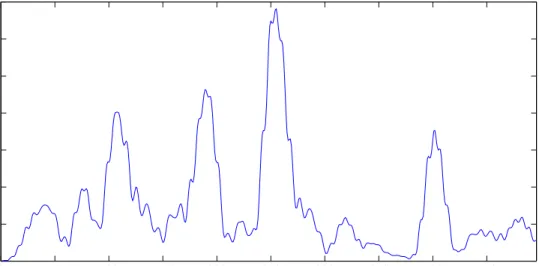
Figure 3.12: DWT decomposition of the EEG signal

3.4.2 WPT

(44)

26 3.4 DWT Based Techniques

Table 3.2: Bands obtained using WPT Frequency (Hz) Related and

The amount of samples for each band is the same and is equal to the number of samples in the last decomposition level of a DWT of the same level. The resulting power signal from the decomposition is shown in Figure 3.13.

0 100 200 300 400 500 600

(45)

3.4.3 Comparison

Fugure 3.14 shows a comparison between DWT and WPT.

0 100 200 300 400 500 600

Figure 3.14: Comparison of DWT and WPT

Both plots show very similar results with small differences in the two upper bands. Just as expected, the two lower bands look identical since the signal goes through the exact same filters, the approximation and detail coefficients for the last level are common for DWT and WPT as it can be noticed by looking at Figures 2.6 and 2.7. The two upper bands do not differ much, they provide the same information but differently distributed because of differences in frequency resolution between techniques as it can be appreciated in Tables 3.1 and 3.2. Since both approaches provided similar results and because DWT is considerably less complex to implement than WPT, it is the last selected technique.

3.5 Comparison between techniques

(46)

28 3.5 Comparison between techniques

4 Alpha Band Power from DWT/WPT

Sample

Power (pW)

Figure 3.15: Comparison of filter and DWT based techniques

The power computed for the FIR is made up of 512 samples and it includes frequencies from 0.5 to 4 Hz. The DWT/WPT approach is made up of the first 38 samples of the output array corresponding to the Alpha band and it includes frequencies from 0 to 5 Hz because of the resolution of the method. Even thought there are differences in resolution and frequency ranges, both plots appear to provide similar information. Scale differences are due to variations in the gain of the filters.

FFT approaches work in the frequency domain and they can not be compared directly to the rest. One way to compare this approach with the other two is to move the time signals computed with the filters and DWT to the frequency domain by calculating PSD. Figure3.16 shows a comparison of PSD for each approach.

0 2 4 6 8 10 12 14 16

(47)

(48)

(49)

Chapter 4 Hardware Platform and Measurement

Procedure

Before running into implementations it is important to set a procedure to ensure that the techniques can be properly evaluated. This chapter provides a brief introduction about the platform under use and its main characteristics. It also estates the procedure to follow in order to measure execution time, memory usage and power consumption.

4.1 Platform Overview

The platform in which the selected feature extraction techniques will be implemented is a MSP432P401R LaunchPad from Texas Instruments. This development kit incorporates a MSP432P401R microcontroller oriented to develop high performance applications that benefit from low-power operation. The main features of this microcontroller are:

• Processor: 48 MHz 32-bit ARM Cortex M4F with FPU and DSP acceleration. • Power consumption: 80 uA/MHz active and 660 nA RTC standby operation. • Analog: 24 Ch 14-bit differential 1MSPS SAR ADC, 2 comparators.

• Digital: Advanced encryption standard accelerator, CRC, DMA, HW MPY32. • Memory: 256 KB Flash, 64 KB RAM.

• Timers: 4 x 16-bit, 2 x 32-bit.

• Communication: up to 4 I2C, 8 SPI, 4 UART.

(50)

32 4.2 Measurement Procedure

The LaunchPad also includes an on-board emulator which means the user can program and debug the projects without the need for additional tools. Free software development tools are available to work with this platform such as the Code Composer StudioTM_(CCS) IDE, IAR Embedded WorkbenchTM IDE and Keil R _µ_Vision R _IDE.

The use of this platform together with the mentioned development tools provides the developer many optimization tools and possibilities to improve any application in terms of code size, speed and mostly low-power consumption. More information about the platform can be found in [14].

4.2 Measurement Procedure

Here, a procedure to measure execution time, memory usage and power consumption is presented. This procedure is not exclusive for the feature extraction techniques and can be used in any application that runs in the MSP432P401R LaunchPad. Each procedure was developed using CCS.

4.2.1 Execution Time

Execution time is, as it name implies, the time it takes to run a piece of code. Measuring execution time with CCS is fairly simple. The measurement can be performed using the debugger by setting breakpoints between the piece of code that wants to be measured and one count event breakpoint, then running the code and finally looking at a counter with the clock cycles that it took the code to run. Then, it is possible to get the execution time if the operating frequency of the system is known by using:

execution time = clock cycles

clock frequency (4.1)

Figure 4.1 depicts an example of the Breakpoints tab showing the clock cycles that it took to run a piece of code and also the two breakpoints that delimit the measured code. The clock cycles for the same piece of code do not vary and therefore the execution time is strictly tied to the operating frequency as shown in Equation 4.1.

(51)

The procedure to measure execution time for a piece of code is:

1. In CCS enter the Debug Mode.

2. Open the Breakpoints tap and create a new count event breakpoint configured to count clock cycles.

3. In the breakpoint properties set reset count on run as true. 4. Place two breakpoint between the piece of code to be measured. 5. Run the program until reaching the last breakpoint.

6. Get the clock cycles from the count event breakpoint. 7. Calculate the execution time.

4.2.2 Memory Usage

As mentioned before, the MP432P401R microcontroller has 256 KB of Flash and 64 KB of RAM, both types of memory have different purposes. Flash memory is non-volatile and it normally stores data that does not change, it is the program memory. RAM memory is volatile and stores data needed at runtime, this memory is very fast but its size is often limited. Two important components of the RAM are the stack and the heap. The stack is the region in RAM in which variables created inside the functions called by the program are stored and the heap is the region of RAM managed by the programmer.

CCS counts with a Memory Allocation tool that makes measuring Flash memory usage fairly simple and is also able to measure RAM memory usage partially. The tool is only able to perform a static analysis on the code and therefore is able to measure static but not dynamically allocated memory.

(52)

Figure 4.2: CCS Memory Allocation tab

If the total RAM memory usage wants to be calculated the programmer needs to include the dynamic allocated peak memory that could be reached by the code and therefore must specify in the build settings the space provided for the heap and the stack. The programmer is the responsible of taking and releasing memory commonly using functions

like malloc and free. To estimate the dynamic peak memory, the programmer should

have a clear idea about what the code does and needs to find the scenario in which the biggest amount of memory is requested. This should not be an issue since every time memory is requested the size of the memory block needs to be specified, so this amount of memory can be approximated by looking at memory allocations inside the code and their respective size.

The procedure to measure memory usage is:

1. In CCS open the Memory Allocation tab.

2. Get Flash memory usage from the MAIN measurement.

3. Get RAM memory usage from the SRAM DATA measurement.

4. Add the amount of dynamically allocated peak memory to the RAM measurement if necessary.

4.2.3 Power Consumption

(53)

EnergyTraceTM _{is an energy based code analysis tool included in CCS that measures} and displays the application’s energy profile and helps to optimize it for ultra-low-power consumption [13]. For MSP432 devices Energy Trace supports two modes of operation: ET (energy profiling only) and ET+ (energy profiling + program counter trace). ET enables analog energy measurements to determine the consumption of an application. ET+ in addition supports a tool useful for measuring and viewing the application’s energy profile and correlating it with the state of the CPU.

Figures 4.3, 4.4 and 4.5 show the different views available for the Energy Trace working in ET mode. For every measurement the user can specify the length of the measurement and is also able to save data for future comparison. The Profile tab provides information about the consumed energy, power, voltage, current and also gives an estimate of the battery life for the current application using a specific type of battery that can also be configured. Power and energy tabs show a plot of how power and energy behave over time for the current application. Sometimes, if the code runs only once and very fast, Energy Trace may not able to measure power. Then, it is useful to include the code that wants to be measured inside a loop just for measuring purposes. By doing that the mean energy consumption for one iteration can be found using:

mean energy = mean power×execution time (4.2)

(54)

Figure 4.4: Power tab in ET mode

Figure 4.5: Energy tab in ET mode

(55)

Figure 4.6: Profile tab in ET+ mode

(56)

For measurement purposes, only ET mode will be used in order to measure power and energy for each technique. Also, each technique was included inside a loop and therefore to measure energy Equation 4.2 was used. ET+ mode can be useful in the final stages of the IoT EEG device when not only feature extraction is ready but the preprocessing and classification stage are too. It could give the chance then to incorporate low-power modes between the acquisition of the signal and the whole processing and can also provide information about the power consumption of each individual stage.

The procedure to measure power consumption is:

1. In CCS a open debug session and open Energy Trace. 2. Configure the time for the measurement.

(57)

Chapter 5 Implementation of Feature Extraction

Techniques

This chapter explains the approach taken for the microcontroller implementation of each feature extraction technique. It introduces the CMSIS-DSP library and describes some of the functions that were borrowed from this library into the implementation. It also brings a detailed explanation of the procedure followed by each algorithm and it presents validations for each technique against the simulated references developed in MATLAB.

5.1 CMSIS DSP Software Library

Before describing the implementation of each feature extraction technique, it is necessary to briefly introduce the CMSIS-DSP Software Library [3]. CMSIS stands for Cortex Microcontroller Software Interface Standard and it is a vendor-independent hardware abstraction layer for the Cortex-M processor series. The CMSIS enables consistent device support and simple software interfaces to the processor and the peripherals. Hence, it is intended to simplify software re-use, reduce the learning curve for microcontroller developers and also the time to market for new devices.

One component of the CMSIS is the CMSIS-DSP. DSP is a library collection with over 60 functions for various data types like fix-point (fractional q7, q15, q31) and single precision floating-point (32-bit). The library is available for all Cortex-M cores. The Cortex-M4 and Cortex-M7 implementations are optimized for the SIMD instruction set. The library covers functions for the following operations:

• Basic math functions. • Fast math functions. • Complex math functions.

(58)

40 5.1 CMSIS DSP Software Library

• Filters.

• Matrix functions. • Transforms.

• Motor control functions. • Statistical functions. • Support functions. • Interpolation functions.

Some functions from filters, complex math functions and transforms were exploited during the implementation of the feature extraction techniques. A short description each of them is given next:

• arm fir init f32: this function is used to initialize a floating-point FIR filter. Here a floating-point FIR filter structure is referenced, also information about the filter coefficients and the size of the block that is processed per call is provided.

• arm fir f32: this function performs a floating-point FIR filtering. It must be called

after the initialization. A FIR instance is provided, a pointer to the input and output vector, and the block size.

• arm rfft fast init f32: this function initializes the floating-point real FFT. Here a

real FFT instance structure is referenced as well as the length of the FFT. It verifies that the length of the FFT is a supported value. Supported FFT lengths are 32, 64, 128, 256, 512, 1024, 2048 and 4096.

• arm rfft fast f32: this function performs a floating-point real FFT. It must be called after the initialization. A FFT instance is provided, also a pointer to the input and output array, and a flag to indicate if a direct or an inverse transform is performed.

• arm cmplx mag f32: this function can compute the magnitude of a floating-point

complex vector. A pointer to the input and output vectors must be provided as well as the number of complex samples in the input.

• arm conv f32: this function computes convolution of floating-point sequences. A

(59)

5.2 Microcontroller Implementation

FIR, Welch’s method and DWT were implemented in the MSP432P401R LaunchPad. For each technique, a general description, implementation details and a performance validation is given. To validate that each technique works as intended, the test signal in Figure 3.1 was also provided to each code as input. The output array was extracted from the microcontroller and then imported to MATLAB in order to be compared to the reference obtained during simulations.

5.2.1 FIR Feature Extraction

The FIR feature extraction implemented code is able to take an EEG input signal to compute power in any of the frequency bands. A single function was developed in which the user must provide an array with the EEG reading, an array containing the filter coefficients for the desired band and finally an output array to store power. The filter coefficients for each band are fixed for a specific sampling frequency and can be easily obtained using MATLAB. Figure 5.1 shows the approach taken to extract features from an EEG reading using FIR.

FIR filtering

Power computation

Moving average filtering

Figure 5.1: FIR feature extraction algorithm sequence

The first step involves filtering the EEG signal. Here, two functions from the CMSIS-DSP are used together. The arm fir init f32 is used to initialize the filter with the provided band coefficients and later the arm fir f32 function computes the filtered signal.

(60)

42 5.2 Microcontroller Implementation

Figure 5.2 shows a comparison of the reference simulated signal from the one obtained in the microcontroller. Since both plots look very similar a plot of the percentage error is provided in Figure 5.3 and also Table 5.1 shows the minimum, average and maximum error in the measurement for the Alpha band and the rest. This measurements show that the algorithm performs well and is able to extract power from each of the bands in a proper and accurate way.

Reference Alpha Band Power (8 Hz − 13 Hz)

Sample

Microcontroller Alpha Band Power (8 Hz − 13 Hz)

Sample

Power (pW)

Figure 5.2: Simulated and microcontroller implementation comparison for FIR

0 50 100 150 200 250 300 350 400 450

−3 Alpha Band Power Percentage Error

Sample

Magnitude

(61)

Table 5.1: Validation percentage error for FIR

Band Minimum Average Maximum

Delta 0.000057911 0.00046846 0.0012616 Theta 0.0000061622 0.001232 0.0060379 Alpha 0.00000046394 0.00051055 0.0031324

Beta 0.000010121 0.028568 1.6774

5.2.2 Welch’s Method Feature Extraction

The implemented Welch’s method algorithm takes an EEG input signal and computes PSD. For this technique a single function was created too, the user must provide an input array containing the EEG reading and an output array that will hold power. For this algorithm the sampling frequency must be declared since it is used for computing the periodogram. The window length, the FFT length and the number of windows are set by the code based on the input size but they can also be tuned for other specific implementations. The code is restricted to work with inputs and windows containing a power of 2 number of elements because of a restriction of the FFT functions from the CMSIS-DSP library. The implemented code creates 7 windows with sizes that are equal to the input size divided by 4, therefore the output will have a size equal to the input size divided by 8 as a result of the periodogram calculation. Figure 5.4 shows the approach taken to extract features from an EEG reading using Welch’s method.

Signal windowing

FFT computation

Periodograms computation

Periodograms averaging

(62)

The first thing to do when using Welch’s method is to apply a window function to the input signal. In this case, a rectangular window function was chosen in order to reduce complexity. A rectangular function window is equal to 1 inside an interval and equal to 0 elsewhere as shown in Figure 5.5, therefore it only implies dividing the signal into intervals. A 50% overlap was selected for the time windows, this makes easier to window the signal and also ensures that every windows will contain a power of 2 number of elements if the input signal does too. This part of the algorithm fills arrays with signal windows to compute FFT later.

1

Time (s) Magnitude

Figure 5.5: Rectangular window

For the FFT computation stage the algorithm takes the windows in which the signal was divided and computes a FFT in each of them. In order to do that, three functions from the CMSIS-DSP library were used. The arm rfft fast init f32 function is used to ensure that the length of the transforms that will be calculated are supported values, if the value is correct the code can execute but if not it will get in an infinite loop. Then,

the arm rfft fast f32 function performs a real floating-point FFT creating an array with

complex values representing each window in the frequency domain. Finally, since the FFT returns a frequency domain representation array with complex values, the magnitude is calculated using the function arm cmplx mag f32.

Having calculated the FFT of each window section it is possible then to compute the periodogram for each block. This is achieved by using Equation 2.4 where the FFT is already computed, the space between samples is the inverse of the sampling frequency and the number in samples is equal to the length of the window.

The final step in Welch’s method is to average all the periodograms. In order to do that, the algorithm adds the same element for each window and divides the result by the number of windows. The output will then be a representation of the PSD in the EEG signal in which all the different bands can be extracted and analyzed.

(63)

0 10 20 30 40 50 60 −140

−120 −100 −80

Reference Power Spectral Density

Sample

Magnitude (dB/Hz)

0 10 20 30 40 50 60

−140 −120 −100 −80

Microcontroller Power Spectral Density

Sample

Magnitude (dB/Hz)

Figure 5.6: Simulated and microcontroller implementation comparison for Welch’s method

0 10 20 30 40 50 60

0 0.5 1 1.5 2 2.5 3 3.5x 10

−4 Power Spectral Density Percentage Error

Sample

Magnitude

Figure 5.7: Validation error for Welch’s method

Table 5.2: Validation percentage error for Welch’s method

Minimum Average Maximum

(64)

5.2.3 DWT Feature Extraction

The algorithm developed to extract features using DWT is able to decompose an EEG signal through a set of high-pass and low-pass filters in order to extract the frequency bands to compute their power. It also provides a bookkeeping vector that indicates the size of the decompositions in order to make easier to extract the bands later. The use of the technique was reduced to a simple function in which the user must provide the input array containing the EEG signal, an output array to store the decomposition and another one to store the bookkeeping vector. The level of decomposition must be declared by the user depending on the specific application. The algorithm uses a db4 mother wavelet by default, the coefficients of both the high-pass and the low-pass filter were obtained using MATLAB. The user can also declare another mother wavelet by changing the arrays holding the coefficients if necessary. Figure 5.8 shows the approach taken to extract features from an EEG reading using DWT.

Bookkeping vector computation

DWT computation

Rearragement of coefficients

Power computation

Figure 5.8: DWT method feature extraction algorithm sequence

(65)

level size = previous level size + filter length - 1

2 (5.1)

After the length of each decomposition level is computed, a small rearrangement is carried out in order to get the bookkeeping vector that contains information of the approximation and detail coefficients for the last level. The detail coefficients for the rest and finally the input size as shown in Figure 5.9.

Length

A = n level approximation coefficients

D = n level detail coefficients

Figure 5.9: Bookkeeping vector structure for DWT

The DWT computation stage is the most relevant in which the frequency bands are extracted. There is no function in CMSIS-DSP library to perform a DWT decomposition as there is for FIR filtering or FFT computation so most of the implementation was developed from scratch. However, the arm conv f32 function from the library was used to make the convolution between the signals in the levels and the filter coefficients. The piece of code that is oriented to compute DWT is embedded inside a loop that runs as many times as level are in the decomposition. It takes the EEG reading as input for the first iteration and then the approximation coefficients of each level for the rest. The first step is to take the input array and pass it thought the filters, it is achieved using the function arm conv f32 between the input and the filters. The result of the convolution is down-sampled to get rid of the extra information since half of the frequencies are cut because of the filter, in order to do that two new arrays store only the odd index values from the approximation and detail coefficients. Both coefficients arrays are stored in one bigger array that stores the whole decomposition because the approximation coefficients need to be used in the next iteration and the details coefficients will be present in the output array. Then the process is repeated until reaching the last level.

(66)

A = n level approximation coefficients

D = n level detail coefficients

n th

Figure 5.10: Rearrangement of coefficients process for DWT

Finally, the last step is power computation. The output vector will hold a set of coefficients representing information about the signal in different bands and power can be extracted from them. In this case power is computed taking the square of the signal representing each band, therefore power is also normalized for this technique.

The simulated reference signal and the microcontroller implementation are compared in Figure 5.11, also the obtained bookkeeping vector is shown in Figure 5.12. Since it is hard to notice differences between the reference and the implementation, a plot of the percentage error is provided in Figure 5.13 and Table 5.3 provides information about the minimum, average and maximum error in the measurements. The error is bigger in samples that show less power but even though this technique shows bigger errors than the others, those errors are still very low. Therefore, from the experimental measurements, it is evident that the developed algorithm is able to decompose an EEG signal using DWT achieving the same results with the MATLAB analysis.

0 50 100 150 200 250 300 350 400 450 500

(67)

1 2 3 4 5 6 0

100 200 300 400 500 600

Bookkeeping Vector

Element

Magnitude

Figure 5.12: Implemented bookkeeping vector for DWT

0 50 100 150 200 250 300 350 400 450 500

0 0.2 0.4 0.6 0.8 1 1.2 1.4

Power Percentage Error

Sample

Magnitude

Figure 5.13: Validation error for DWT

Table 5.3: Validation percentage error for DWT Minimum Average Maximum

(68)

50 5.3 Optimizations

5.3 Optimizations

Each technique was not only implemented but also optimized as much as possible in order to improve execution time, memory usage and power consumption before running the evaluations. The selected optimizations and also results that demonstrate their impact are shown for each technique. Every measurement was carried out using the procedures described in Chapter 4.

5.3.1 Execution Time and Memory Usage

CCS incorporates optimization tools and options to improve speed, code size and power consumption. Settings in the compiler can be adjusted to achieve different optimization levels for speed and code size. Figure 5.14 shows the optimization view in CCS. There are different optimization levels that can be selected from 0 to 4, these optimizations can include register, local, global, interprocedure and whole program optimizations. There are two floating point modes, strict is the one set by default and relaxed is another mode that results in smaller and faster code by sacrificing some accuracy. Finally, there is another option to select the trade-off between speed and code size from 0 to 5, being 0 oriented to size and 5 to speed.

Figure 5.14: Compiler optimization view

(69)

Figure 5.15: Code size for different optimization level settings

Figure 5.16: Code size for different code size and speed trade-off settings

The Optimizer Assistant was used to determine which was the best combination of settings for each technique. Table 5.4 contains the optimization settings used for each technique using the Optimizer Assistant.

Table 5.4: Compiler optimization settings

Technique Optimization level

Floating point mode

Speed vs size trade-off

FIR 4 Relaxed 2

Welch’s method 4 Relaxed 2

DWT 3 Relaxed 2

(70)

Table 5.5: Speed (clock cycles) optimization

Technique Before

Table 5.6: Code size (bytes) optimization

Technique Before

Power consumption was also optimized for each feature extraction technique. Operating voltage and frequency are critical parameters in power consumption. In this case, both parameters were tuned in order to find the most suitable parameters combination. Given that power is the product of voltage and current, if there is an application that consumes a certain amount of current, a lower supply voltage can help reduce the power consumption. The MSP432P01R requires a secondary core voltage (VCORE) for its internal digital operation in addition to the primary one applied to the device (VCC). The VCORE output is programmable with two predefined voltage levels. VCORE0 is approximately 1.2 V and is recommended for applications running in frequencies bellow 24 MHz while VCORE1 is close to 1.4 V and is recommended if the operating frequency is between 24 MHz and 48 MHz.

(71)

As it was also mentioned, the selection of the operating frequency of the system is an important element in low-power consumption applications. A reduction in the operating frequency will cause a reduction in current consumption. However, reducing the frequency could reduce overall system throughput or may increase energy consumption. Energy is the product between power and time, therefore there is a possibility that the same code can consume more power but less energy at higher frequencies because the power is consumed during a shorter period of time.

Since the selection of the VCORE is strictly tied to the operating frequency, for each of the feature extraction technique different frequencies and hence operating voltages were evaluated to get the power and energy consumption. Because the application requires to reduce energy consumption as much as possible, the DC-DC regulator was selected over the LDO.

Tables5.7and Figure 5.17show the results of the measurements for power in five different frequencies, starting in the 3 MHz default frequency up to the maximum of 48 MHz. Just as expected it can be seen that power consumption rises when frequency does.

Table 5.7: Power (mW) measurements for optimization

Technique Frequency (MHz)

3 12 24 36 48

FIR 10.49 11.62 13.58 17.43 20.07 Welch’s method 10.20 11.60 13.60 17.53 19.96 DWT 9.43 11.06 13.40 17.29 20.12

0 5 10 15 20 25 30 35 40 45 50

(72)

Based only on the power readings the ideal frequency to choose use would be the lowest, however as mentioned before, a low frequency produces a slower execution and therefore it consumes power for more time. It is necessary then to measure not only power but also the time for how long power is consumed to estimate energy. Looking at the energy plot in Figure5.18 energy consumption goes down as frequency increases. It means that even though more power is consumed at higher frequencies, it is consumed for a shorter time period. Based on these experiments the selected operating frequency is 48 MHz and the core voltage setting VCORE1.

Table 5.8: Energy (uJ) measurements for optimization

Technique Frequency (MHz)

3 12 24 36 48

FIR 5336.84 1477.93 863.61 738.97 638.17 Welch’s method 789.55 224.48 131.59 113.08 96.57 DWT 779.85 228.54 138.45 119.09 103.94

0 5 10 15 20 25 30 35 40 45 50

Figure 5.18: Energy measurements for optimization

(73)

Chapter 6 Evaluation of Feature Extraction

Techniques

After exploring, simulating and implementing different feature extraction techniques, it is possible to evaluate them and analyze how each would fit in an IoT implementation of an EEG. Execution time, memory usage and power consumption are measured and compared in order to find how the selected techniques perform not only in each specific parameter but also taking them as a whole, keeping in mind that the EEG device should face computation capability and energy capacity in the best way possible. In order to evaluate the techniques in equal conditions, the test signal in Figure 3.1 was provided to each code as input. Every measurement was taken following the procedures explained in Chapter 4.

6.1 Execution Time

CPU cycles were measured and time was computed using Equation 4.1. The 48 MHz operating frequency defined during the optimization was also set. Table 6.1 and Figure 6.1 show the results of the execution time measurements for each algorithm.

Table 6.1: Execution time evaluation

Technique CPU cycles Time (ms)

FIR 1526264 31,80

Welch’s method 232221 4,84

DWT 247968 5,17

Evaluation of Feature Extraction Techniques for an Internet of Things Electroencephalogram