The role of urban vegetation in temperature and heat island effects in
Querétaro city, Mexico
MARÍA L. COLUNGA, VÍCTOR HUGO CAMBRÓN-SANDOVAL, HUMBERTO SUZÁN-AZPIRI, AURELIO GUEVARA-ESCOBAR and HUGO LUNA-SORIA
Facultad de Ciencias Naturales, Universidad Autónoma de Querétaro, Avenida de las Ciencias s/n, Juriquilla, 76230 Querétaro, México
Corresponding autor: H. Suzán-Azpiri; e-mail: [email protected]
Received: November 13, 2013; accepted: June 24, 2015
RESUMEN
La alteración de las condiciones climáticas y el efecto de isla urbana de calor (EIC) son resultado del incre-mento de la población y de sus actividades en las zonas urbanas. En ciudades medianas como Querétaro es importante determinar la magnitud del EIC y promover la planeación del crecimiento urbano. Conservar y aumentar las áreas con vegetación es una buena opción para mitigar el EIC. En este estudio se analizaron la intensidad del EIC y el efecto de la cobertura vegetal sobre la regularización de la temperatura del aire. Se
parcela de medición en la cual se consideraron dos niveles de cobertura vegetal en función del índice de área foliar: bajo y alto (0.5 y 2.0, respectivamente). La temperatura del aire se midió con recolectores de datos a intervalos de 30 min entre junio de 2012 y mayo de 2013. También se analizaron datos climáticos de seis estaciones meteorológicas. La temperatura media diaria aumentó a razón de 0.75 ºC por década (r2 = 0.38, P < 0.0001); este aumento se relacionó con la dinámica poblacional (r2 = 0.52, P < 0.0001). Los patrones estacionales de temperatura se describieron como temporada fría de julio a marzo y temporada cálida de abril a junio para la temperatura máxima, y temporada fría de noviembre a marzo y temporada cálida de abril a octubre para la temperatura mínima. La diferencia entre las temporadas cálida y fría fue del orden de 5 ºC (
de la vegetación. Sin embargo, la humedad relativa fue mayor en el nivel alto de la cobertura vegetal. La
La intensidad del EIC fue similar para la temporada cálida y fría y varió de 0.1 a 5 ºC. La vegetación con mayor cobertura presentó menor temperatura a las 17:00 horas y mayor de las 9:00 a las 10:00 horas durante la temporada cálida. Al aumentar 50% la cobertura vegetal en la zona urbana se lograría reducir la intensidad del EIC en 2.05 ºC. En conclusión, una mayor cobertura de la vegetación mejora las condiciones ambientales en términos de humedad relativa y regularización de los extremos de temperatura durante la temporada cálida.
ABSTRACT
Alteration of climatic conditions and the urban heat island effect (UHI) are consequences of increased human population and activities in urban zones. Determining the magnitude of the UHI is important to improve urban planning in medium-size cities like Querétaro. Increase and conservation of vegetated areas is a mitigation option for UHI. Here we characterized both the UHI and the role of vegetation cover over temperature
reg-temperature and relative humidity were measured with data loggers at a 30 min time step from June 2012 to May 2013. Climatic data from six weather stations was also analyzed. Daily mean temperature increased at a rate of 0.75 ºC per decade (r2 = 0.38, P < 0.0001), and this was related to population dynamics (r2 = 0.52,
for maximum temperature, and November to March and April to October for minimum temperature. The difference between cold and warm seasons was 5 ºC (P < 0.0001). The minimum temperature was similar
© 2015 Universidad Nacional Autónoma de México, Centro de Ciencias de la Atmósfera.
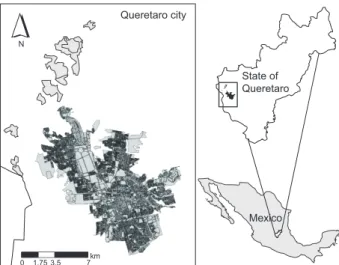
Mexico State of Queretaro Queretaro city
N
0 1.75 3.5 7kmkm
Fig. 1. Geographic location of the study area (Querétaro City).
between canopy cover levels. However, relative humidity was higher in high canopy cover plots. The re-lationship between UHI and the pervious surface fraction of the city was inversely proportional. The UHI ranged from 0.1 to 5 ºC and this magnitude was similar between the warm and cold seasons. Vegetation with high canopy cover had lower temperature at 17:00 LT and higher at 9:00 to 10:00 LT during the warm season. Increasing the urban zone canopy cover by 50% would reduce the UHI by 2.05 ºC. In conclusion, vegetation with higher canopy cover improved environmental conditions in terms of relative humidity and regularization of extreme temperatures during the warm season.
Keywords: Climate change, urban heat island effect, urban planning, Querétaro, vegetation.
1. Introduction
According to the population report of the United Na-tions (2014), 54% of human population lives in urban areas and it is increasing at a rate of 1.8% per year. By year 2050 rural population would decrease to one third of its present size. Urban concentration of human
population causes deep modifications in the city and
its surrounding landscapes, affecting environmental and climatic conditions (Yu and Hien, 2006; Um et al., 2007). The effect and dynamics of the urban heat island (UHI) are well-known and deeply studied cli-matic processes (García-Cueto et al., 2007; Doick and Hutchings, 2013). The UHI effect is described as the difference in environmental temperature between the urban area and its rural periphery (Oke, 1973; Stewart, 2011; Li et al., 2013). The variation of air temperature associated with the UHI intensity depends on factors such as infrastructure and building design and density, among many others (García-Cueto et al., 2009; Li et al., 2013). Compared to the countryside, the low al-bedo and high heat absorption of city surfaces (Doick and Hutchings, 2013), coupled with the generation of greenhouse gases (GHG) and dust from industrial processes and anthropogenic activities (Wilby, 2003; Hunt et al., 2007), contributes to the increase in air
temperature, and modifies surface wind flow and air
quality (Blake et al., 2011; Doick and Hutchings,
2013).
The increase of vegetation areas is a main option explored to mitigate UHI (Anyanwu and Kanu, 2006; Li et al., 2013). Urban vegetation regulates
climate mainly by shading (Emmanuel, 2005), CO2
sequestration (Lin et al., 2011) and evapotranspira-tion (Yu and Hien, 2006). The mitigaevapotranspira-tion potential of urban vegetation needs additional research because native vegetation and climate are strongly related, and this types of plants should be preferred as a ro-bust mitigation option; nevertheless, exotic trees are common in the urban context.
In this paper, we analyzed the UHI for Querétaro City, Mexico. This study is an effort of the Programa Estatal de Acción ante el Cambio Climático-Querétaro (State of Querétaro Action Program Addressing Cli-mate Change, PEACC-Q) (Suzán-Azpiri et al., 2014). The aims of this study were to evaluate (1) the role of vegetation in urban temperature regularization, and (2) the role of vegetation cover in the adaptation to UHI effects.
2. Methodology
2.1 Study area
The study area is the city of Querétaro (Fig. 1), locat-ed in the southwestern portion of the State of Queréta-ro, Mexico (20º 35’ 34.8’’ N, 100º 23’ 31.6’’ W).
It covers an area of 759.9 km2 with a population of
Table I. Parameters of geometric and surface cover properties for the LCZs of Querétaro City,
according to the Stewart and Oke (2012) classification.
Properties LCZ B LCZ 6 LCZ 3 LCZ 2
Sky view factor (Ψsky) 0.5-0.8 0.6-0.9 0.2-0.6 0.3-0.6
Aspect ratio (H/W) 0.25-0.75 0.3-0.75 0.75-1.5 0.75-2
Mean height of trees/buildings (zH) (m) 2 13 9 < 20
Terrain roughness class 5 5 6 6
Building surface fraction (λb) (%) 0.11 30.14 58.03 64.39
Impervious surface fraction (λi) (%) 0.14 27.46 26.95 34.28
Pervious surface fraction (λv)(%) 99.75 42.40 15.02 1.33
Surface admittance (μ) (J m–2 s–½ K–1) 1000-1800 1200-1800 1200-1800 1500-2200 Surface albedo (α) (%) 0.15-0.25 0.12-0.25 0.10-0.20 0.10-0.20
Anthropogenic heat flux (QF) (W m–2) 0 < 25 < 75 < 75
LCZ B: scattered trees; LCZ 6: open low-rise; LCZ 3: compact low-rise; LCZ 2: compact mid-rise.
The city of Querétaro can be classified as poly -centric, with main urban cores associated to industrial and commercial areas (Álvarez de la Torre, 2010). The historic downtown is mainly composed of baroque buildings less than six stories tall. Almost 90% of the streets in the center of the city and its surroundings are paved with cobblestone, and the rest have asphalt surfaces. Industrial plots are allotted within industrial parks located to the north, east and southwest of the city; they are main land use chang-es that contribute to urban growth (Icazuriaga and Osorio, 2007). Concrete and steel buildings, as well as asphalt roads, are representative of these areas. Finally, 70% of the households are less than three sto-ries single-family buildings; the rest are multi-family complexes and two level houses of social interest located on the periphery. Concrete, metal, bricks, tiles and polystyrene are the main construction materials on households. The streets are mainly asphalt roads and in some cases they are covered with cobblestone (Aragón and López, 2013).
Using Landsat 8 imagery (Sensor OLI_TIRS_L1T,
December 5,2013, USGS Global Visualization
View-er) we created a supervised classification of the city
using ENVI 5 (ITT Visual Information Solutions). Ap-proximately 65% is constructed; 37% is paved; 28% is covered by vegetation or bare soil; and less than 1%
is occupied by water (dams and artificial reservoirs).
2.2 Study zones
To avoid the arbitrary designation of urban and rural zones (Stewart, 2007), we used the climate-based
classification system developed by Stewart and Oke
(2012). This system describes the local physical
con-ditions around the measuring field sites, classifying
them into local climate zones (LCZs). Four circular zones with a 500 m radius (78.5 ha) (WMO, 2008) were selected randomly within the range of 1 to 99% vegetation cover. We used satellite imagery to estimate the mean height of trees and buildings, the building surface fraction, and the impervious and pervious fractions (Table I). The rest of the values were taken from literature (Oke, 2006; Stewart and Oke, 2012).
The four zones were classified accordingly as scattered
trees (LCZ B), open rise (LCZ 6), compact low-rise (LCZ 3), and compact mid-low-rise (LCZ 2).
2.3 Local climate zones 2.3.1 LCZ B (scattered trees)
Described as lightly dense vegetation comprised by shrubs, cacti (Opuntia sp. and Myrtillocactus geome-trizans), tropical dry forests (TDF) and reforestation patches (i.e. Jacaranda mimosifolia, Eucalyptus globulus). It constitutes one of the best-preserved cli-mate zones in the municipality of Querétaro (Baltazar et al., 2004), and is located in the southern periphery of the city (Fig. 2).
2.3.2 LCZ 6 (open low-rise)
It is composed of one to three stories small buildings of diverse construction materials (concrete, stones, bricks, tiles and metal). Fifty percent of the surface is covered with scattered shrubs and TDF. It has
22027
22004 22006
22070
22063 LCZ 6
LCZ 2 LCZ 3
LCZ B 22045
Simbology
Climatic stations Study zones Main roads Queretaro city
´
227000
02
280000
2290000
227000
02
280000
2290000
350000
340000 360000
350000
340000 360000
Fig. 2. Location of the four delimited local climate zones (LCZ B, LCZ 2, LCZ 3, LCZ 6) and situation of the climatic stations of the Sistema Mete-orológico Nacional (National Meteorological System, SMN) (CNA-SMN, 2014) within the city of Querétaro.
and apartments) and commercial use (small shopping centers). These suburbs are located on the northern periphery of the city.
2.3.3 LCZ 3 (compact low-rise)
A dense mix of low-rise buildings with less than three stories and diverse construction materials (concrete, stone, tiles and bricks). Pavement and cobblestone cover most of the streets with a few scattered trees. It is located within the city core (medium density) and has residential use (single unit households).
2.3.4 LCZ 2 (compact mid-rise)
Dense mix of mid-rise buildings lower than nine stories of diverse construction materials (concrete, stone, tiles, bricks and metal). Most of the streets are covered with pavement and cobblestone, with a few scattered trees (Eucalyptus sp., Ficus sp. and Jacaranda sp.). It is adjacent to the city center and has residential use (scattered single unit households).
2.4 Sampling
In each LCZ we established random sampling points according to two different vegetation cov-er categories: high (+C) and low (–C) (Table II).
The characterization of each category was deter-mined by the leaf area index (LAI), one-sided green
leaf area per unit ground surface (m2/m2). The LAI
was measured using a LAI-2000 Plant Canopy Analyzer (Li-Cor Inc., USA) which evaluates the transmission of light through the canopy in terms of gap fraction. For each LAI data, the average of three measurements under the canopy (separated by one meter each in a north-south direction), and one measurement above the canopy were obtained
(Guevara et al., 2012). For each sampling point
(n = 12), air temperature and relative humidity were measured with a climatic data logger EL-USB-2 (Hobo Pro v.2, LASCAR, USA). The data loggers were programmed to record every 30 min from June 1, 2012 to May 31, 2013.
2.5 Temperature corrections
Heating and cooling of air is considered to be an adi-abatic process responding to the variation in gas pres-sures (Lutgens and Tarbuck, 2012). In this context, air temperature is directly affected by altitude, and we standardized altitude and pressure by an adjust-ment with a Poisson function (Eq. 1). The resulting
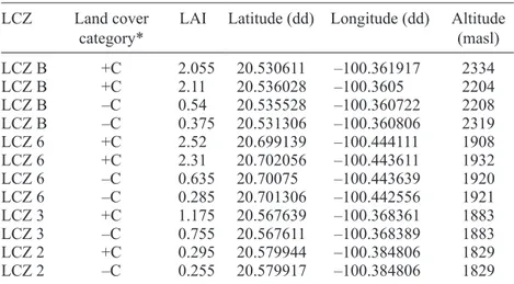
Table II. Leaf area index (LAI), geographic coordinates and altitude values of the sampling points in each local climate zone (LCZ).
LCZ Land cover
category* LAI Latitude (dd) Longitude (dd) Altitude (masl)
LCZ B +C 2.055 20.530611 –100.361917 2334
LCZ B +C 2.11 20.536028 –100.3605 2204
LCZ B –C 0.54 20.535528 –100.360722 2208
LCZ B –C 0.375 20.531306 –100.360806 2319
LCZ 6 +C 2.52 20.699139 –100.444111 1908
LCZ 6 +C 2.31 20.702056 –100.443611 1932
LCZ 6 –C 0.635 20.70075 –100.443639 1920
LCZ 6 –C 0.285 20.701306 –100.442556 1921
LCZ 3 +C 1.175 20.567639 –100.368361 1883
LCZ 3 –C 0.755 20.567611 –100.368389 1883
LCZ 2 +C 0.295 20.579944 –100.384806 1829
LCZ 2 –C 0.255 20.579917 –100.384806 1829
* High (+C) and low (–C). dd: decimal degrees; masl: meters above sea level.
as “the temperature that a parcel of air would have if it were expanded or compressed adiabatically from its existing pressure and temperature to a standard pressure” (Wallace and Hobbs, 2006; Mohanakumar, 2008). Mathematically, it is expressed as:
θ = T
( )
pp0 R/cp (1)where θ = potential temperature, T = original
temperature, p0 = standard pressure of 1000 hPa,
p = original pressure, R = universal gas constant
(287 J K–1 kg–1); and c
p = specific heat constant (1004 J K–1 kg–1).
To calculate the pressure corresponding to tem-perature data we used the hypsometric or barometric equation (Eq. 2), which relates pressure and tempera-ture at a certain atmospheric altitude (Adamson, 2012):
ph = p0 e(–mgh/RT) (2)
where: ph = pressure at h height, p0 = pressure at
ground level (1013.25 hPa), M = the mass or a mole
of particles of air (0.029 kg mol–1), g = gravitational
acceleration (9.8 m s–2), h = height in meters, R =
universal gas constant (8.314472 J K–1 mol–1), and
T = average temperature at height (ºK).
2.6 The role of vegetation in urban temperature dy-namics
In a global scale, a rise in minimum temperature has a greater impact on average daily temperature than
maximum temperature (IPCC, 1997). Therefore, the effects of climate change are mainly detected in minimum daily temperatures (IPCC, 2007). In order to prove this hypothesis within the city of Querétaro we analyzed daily average minimum temperatures
(Tmin, ºC) and maximum temperatures (Tmax, ºC)
between 1982 and 2011 from six climate stations (Table III). Data were obtained from the databas-es of the SMN (CNA-SMN, 2014). In the case of
Querétaro, all stations were previously verified with
the RClimDex software (Zhang and Yang, 2004), developed within the PEACC project (Suzán-Azpiri et al., 2014). Moreover, the databases of the six
sta-tions were filtered to ensure temporal homogeneity
throughout the 30 years. Additionally, we analyzed
the relationship between variations in Tmin and Tmax
as a function of population size, according to the demographic censuses conducted between 1990 and
Table III. Geographic coordinates and altitude values for the seven climate stations of the SMN (CNA-SMN, 2014).
Code Name Latitude
2010 (INEGI, 1990, 2010). Finally, we studied the oscillation in a monthly scale to identify extreme periods in both Tmin and Tmax.
In order to evaluate the role of vegetation cover in urban temperature dynamics, we evaluated the
changes in Tmin and average relative humidity (RH, %)
in function of the different LCZs, canopy cover status (+C and –C) and pervious surface fraction (PSF, %)
–defined as the percentage of vegetated surface–,
between June 1, 2012 and May 31, 2013.
2.7 Vegetation cover and effect of the UHI
According to Stewart and Oke (2012), the UHI is represented as a function of the intensity differ-ence (∆T) between LCZs temperatures according to the degree of urbanization. Mathematically it is
defined as:
UHI= ∆TLCZ x-y (ºC) (3)
where UHI is the intensity of the urban heat island ef-fect, ∆T is the temperature difference between LCZs, LCZx is the zone with more urban components (Table I), and LCZy is the zone with less number of urban components (Table I).
In this study, we quantified the differences be
-tween average minimum temperatures (∆Tmin, ºC)
between the four described climate zones in six pos-sible arrangements: LCZ2-3, LCZ2-6, LCZ2-B, LCZ3-6,
LCZ3-B and LCZ6-B. The role of vegetation in UHI
dynamics was evaluated through the fluctuation in
∆Tmin for the LCZx-y arrangements according to the
cover status (+C y –C), and seasonality (cold and
warm seasons). Additionally, a daily profile of UHI
(24 h) changes was studied.
2.8 Statistical analysis
A linear regression (LR) analysis was applied to eval-uate the annual increase in daily average minimum and maximum temperatures from six meteorological stations, with the function:
Y= β1 + β0X (4)
where Y is the dependent variable (Tmin and Tmax), β1 is
the intercept, β0 is the slope, and X is the independent
variable (year).
In order to estimate Tmin and RHave differences
among the LCZs zones, according to the status of
vegetation cover (+C and –C), a full factorial analysis was performed with the model:
Yijk = m + Mi + Lj + Sk + M*Lij +
M*Sik + L*Sjk + M*L*Sijk + eijk (5)
where µ is the general average value, Mi is the
month-ly effect, Lj is the zone, Sk is the effect for the k-th
status of vegetation, M*Lij is the interaction
month-zone, M*Sik is the interaction month-status, S*Lkj is
the interaction status-zone, M*L*Sijkis the interaction
month-zone-status, and eijk is the random error.
A simple linear regression analysis was applied to
explore the relation between the Tmin and the pervious
surface fraction (PSF, %) (Table I) of the four LCZs with the function:
Y= β1 + β0X (6)
where Y is the dependent variable (Tmin), β1 is the
intercept, β0 is the slope, and X is the independent
variable (PSF).
The monthly changes in the UHI associated to the
status of the cover (+C and –C) in each LCZx-y, were
analyzed with the model:
Yijk = m + Mi + Cj + Sk + M*Cij +
M*Sik + C*Sjk + M*C*Sijk + eijk (7)
where µ is the average value, Mi is the effect for the
i-th month, Cj is the effect for the j-th LCZx-y, Sk is
the effect for the k-th status of vegetation, M*Cij is
the interaction month-LCZx-y, M*Sik is the interaction
month-status, S*Lkj is the interaction status-zone,
M*L*Sijk is the interaction month-zone-status, and
eijk is the random error.
Linear regression analysis was applied to explore the relation between the UHI and the difference
be-tween the pervious surface fraction (ΔPSF, %) in the
six arrangements LCZx-y, with the function:
Y= β1 + β0X (8)
where Y is the dependent variable (ΔTmin), β1 is the
intercept, β0 is the slope, and X is the independent
variable (ΔPSF).
The hourly behavior of the UHI at high and low
temperature phases between the LCZx-y, was
34
32
30
28
26
24
14
12
10
2
1985
c) a)
y = –21.975 + 0.025x r2 = 0.07, P < 0.0001
y = –139.252 + 0.075x
r2 = 0.38, P < 0.0001 y = 7.464 – 6.625e –6x
r2 = 0.52, P < 0.0001
y = 28.619 – 3.598e–7x
r2 = 0.0018, P < 0.0001
d) b)
1990 1995 2000 400 450 500 550 600 650
Population size (thousands) Year
Minimum temperature (º
)M
inimum temperature (º
)
2005 2010
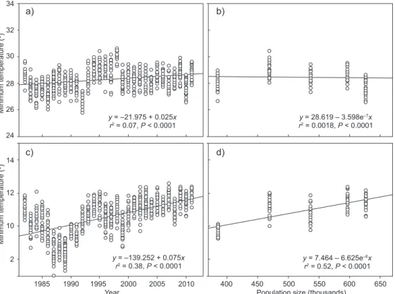
Fig. 3.Scatterplots and linear regressions between daily average temperature on time (a and c) and Querétaro city population size (b and d), from six climate stations of the SMA (CNA-SMN, 2014).
Yij= m +Ei + Hj +E*Hij + eij (9)
where µ is the general average, Fi is the effect of the
de i-th fase, Cj is the effect for the j-th LCZx-y, Hk is the
effect of the j-th hour, F*Cij is the interaction phase
LCZx-y, F*Hik is the interaction phase-hour, C*Hjk is
the interaction LCZx-y-hour, F*C*Hijk is the
interac-tion phase-LCZx-y-hour, and eijkis the random error.
3. Results and discussion
3.1 Historic and annual temperature oscillation The temperature comparison for the period 1982-2011 from six climate stations within the city of
Querétaro showed significant differences between the
daily Tmax (P < 0.0001, F = 49.99, 29, 929) and Tmin
(P < 0.0001, F = 122.53, 29, 900) among the 30 years.
The LR exhibited a low significant linear trend for the
increase in annual Tmax (P < 0.0001, r2 = 0.07) (Fig. 3a).
In contrast, Tmin had a more significant trend
(P < 0.0001, r2 = 0.38) of 0.751 ºC per decade (Fig. 3c). This differential trend agreed with the global pattern, where minimum daily temperatures increase faster than maximums. However, the rate was higher than
the global decadal range (0.254 to 0.273 ºC) between 1979 and 2012 (IPCC, 2013).
This increase was higher than in other Mexican cities, where values of 0.57 ºC for large metropolis (bigger than one million inhabitants) and 0.37 ºC for medium size cities (smaller than one million) are found (Jáuregui, 2005). Particularly the city of Querétaro, with less than one million inhabitants, has experienced a high rate of urban growth (Icazuriaga and Osorio, 2007) of about 33% between 1990 and 2010 (INEGI,
1990, 2010). This growth was significantly correlated
with the daily annual average Tmin increase (r2 = 0.52, P < 0.0001) (Fig. 3d), but not with the Tmax (r2 = 0.0018, P < 0.0001) (Fig. 3b). Therefore, factors related to the urbanization process like the increase in building surface fraction and impervious surface fraction, the change in surface albedo and the rise of anthropogenic
heat flux, could explain the Tmin increase.
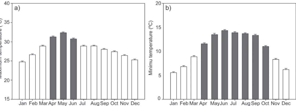
In a monthly scale we detected significant differ -ences in Tmax (P < 0.0001, F = 115.27, 11, 348) (Fig. 4a) and in Tmin (P < 0.0001, F = 180.69, 11, 348) (Fig. 4b).
During the cold season for Tmax (defined as July
Jan Feb MarApr May Jun Jul Aug Sep Oct Nov Dec 0 Jan 5 10 15 20 40
35
a) b)
30
25
Maximum temperature (ºC)20 Minimu temperature (ºC)
15
Feb Mar Apr MayJun Jul Aug Sep Oct Nov Dec
Fig. 4. Monthly average for maximum temperature (Tmax) and minimum temperature (Tmin) between 1982
and 2011 for six climate stations of the SMA (CNA-SMN, 2014). Black bars (warm season) are significantly
different from white bars (cold season). Line bars are the standard errors of the mean.
Fig. 5. Average of minimum temperature (Tmin) for the local
climate zones (LCZ) according to low (–C) and high (+C) canopy cover categories during the cold and warm season described in Fig. 4. Cold: ▼–C, ▲+C. Warm: ▼–C, ▲+C.
Line bars are the standard errors of the mean.
20
18
16
14
12
Tmi
n
(ºC)
10
8
6
LCZ 2 LCZ 3 LCZ 6 LCZ B
27.24 ± 1.58 ºC, while these values during the warm
season for Tmax (April to June) were 31.45 ± 0.85 ºC
(Fig. 4). In contrast, the cold season for Tmin
(Novem-ber to March) had a mean and standard deviation of 7.51 ± 1.40 ºC, while these values during the warm season (April to October) for the same variable were 13.13 ± 1.43 ºC. Both trends in temperature agree with the pattern detected for a larger region in Mexico (Morillón et al., 2002).
3.2 The role of vegetation in urban temperature
For the studied period, average Tmin was 13 ºC with a
maximum of 14.89 ºC and a minimum of 10.79 ºC.
Significant differences between the studied zones were detected (P < 0.0001, F = 85.42, 3, 87). These differences oscillated from 1.6 ºC between LCZ 3 and LCZ 6, to 4 ºC between LCZ 2 and LCZ B. In agreement with Alexander and Mills (2014), the areas with more urban elements such as high
anthropo-genic heat flux percentages, impervious surface and
building surface fraction, had temperatures over the mean (LCZ 2 and LCZ 3), while the less urbanized areas had temperatures below the mean (LCZ 6 and LCZ B). Among the annual seasons, a 5 ºC difference between cold and warm seasons was detected (P < 0.0001, F = 602.93, 1, 87). These results agree
with the findings reported by Romero-Dávila et al. (2011) for the city of Toluca, Mexico.
No significant differences were found between –C
and +C for Tmin (P = 0.80, F = 0.06, 1, 87) (Fig. 5).
However, Yu and Hien (2006) proved that foliar density (LAI) within a green area has an effect on air temperature; particularly in urban gardens, high
values in the LAI (> 7) were associated with lower temperatures. Therefore, we deduced that the differ-ence between +C and –C for each climate zone was
insufficient to detect an effect on Tmin.
70
65
60
55
50
RH (%
)
45
40
35
LCZ 2 LCZ 4 LCZ 6 LCZ B
Fig. 6. Average of relative humidity (RH) for local climate
zones (LCZ) during the cold (○) and warm (●) seasons
as described in Fig. 4. Line bars are the standard errors of the mean.
20
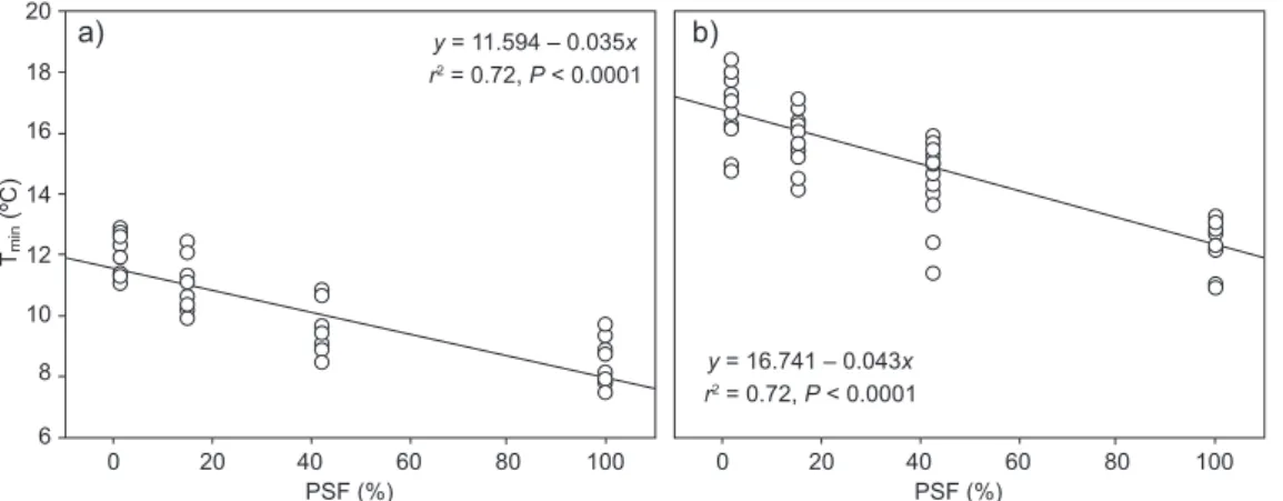
a) y = 11.594 – 0.035x
r2 = 0.72, P < 0.0001
y = 16.741 – 0.043x r2 = 0.72, P < 0.0001 b)
18
16
14
12
10
8
6
0 20 40
PSF (%)60 80 100 0 20 40PSF (%)60 80 100
Tmi
n
(ºC)
Fig. 7. Relationship between monthly average minimum temperature (Tmin) and pervious surface
fraction (PSF) of the four local climate zones during (a) cold and (b) warm seasons, as described in Fig. 4.
The relationship between PSF and Tmin was
sig-nificant for the cold and warm seasons (r2 = 0.72, P < 0.0001). According to the equation’s model of lin-ear regression (Fig. 7a and 7b), a 50% increase in PSF produced a decrease of approximately 1.75 and 2.18 ºC
in Tmin for both seasons. Yan et al. (2014)
demon-strated a similar relationship between canopy cover and temperature in urban parks; an increase of 50% in vegetation cover produced a decrease of 0.6 ºC in air temperature, reinforcing the idea that canopy cover is a regulator of environmental temperature (Yu and Hien, 2006; Li et al., 2013).
According to Wilby (2003) and Lin et al. (2011), through evapotranspiration vegetation acts as an
evaporative cooling system, creating an albedo 15% higher than urban surface due to smaller heat
absorp-tion and higher reflected radiaabsorp-tion (Doick and Hutch -ings, 2013). Also, the shade effect decreases incident radiation and the micro greenhouse effect within buildings (Emmanuel, 2005; Anyanwu and Kanu, 2006), which promotes energy savings by decreasing the demand in cooling systems; it also reduces health risks by decreasing atmospheric pollutants while
in-creasing CO2 sequestration (Lin et al., 2011).
3.3 Effect of the urban heat island (UHI)
Significant temperature differences were found be
-tween LCZ2-B and LCZ3-6 (P < 0.0001, F = 155.88,
5, 120; Tukey-Kramer α = 0.05, Q = 2.89), with a 4.94 ºC maximum intensity and a 0.48 ºC minimum intensity (Fig. 8). Alexander and Mills (2014) found
similar results between LCZ2-D (4.8 ºC). During the
warm season an UHI of 2.64 ºC in average, with a 5 ºC maximum and a 0.82 ºC minimum, was detected. In the cold season, UHI values had a 2.46 ºC average, ranging from a 4.88 ºC maximum to a 0.14 ºC minimum. These values agreed with the maximum UHI reported for the city of Mexicali, Mexico; 5.4 ºC during the summer (García-Cueto et al., 2007) and 4.5 ºC during winter (García-Cueto et al., 2009); and also for Toluca, Mexico with values of 5 ºC for winter and summer (Romero-Dávila et al., 2011). There was no effect of the canopy cover (–C and +C) over UHI intensities (P = 0.2073, F = 1.60, 1, 120).
The relationship between the UHI and the
6
5
4
3
2
UHI (ºC)
1
0
2-3 3-6 2-6
LCZ x-y6-B 3-B 2-B –1
Fig. 8. Urban heat island (UHI) intensity of monthly
aver-age minimum temperature (ΔTmin) between local climate
zones (LCZs), during cold (○) and warm (●) seasons as
described in Fig. 4, where x and y represent more and less urbanized zones, respectively. Line bars are the standard errors of the mean.
7
a) b)
6
5
4 3
UHI (ºC) 2
1
0
–1
∆PSF(%) 0 20 40∆PSF(%)60 80 100
0 20 40 60 80 100
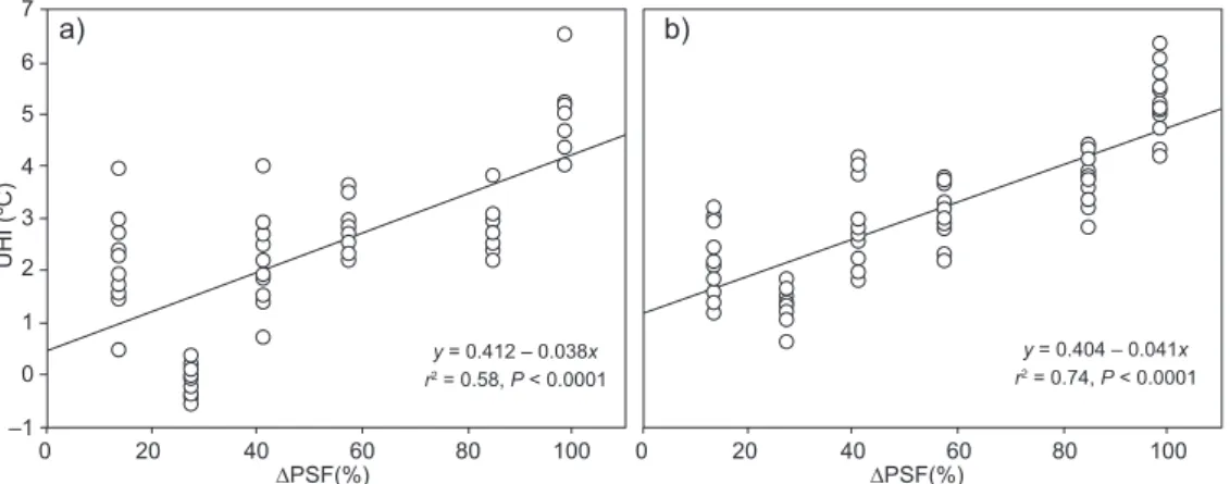
y = 0.412 – 0.038x r2 = 0.58, P < 0.0001
y = 0.404 – 0.041x r2 = 0.74, P < 0.0001
Fig. 9. Relationship between urban heat island (UHI) intensity and difference in the pervious surface fraction (ΔPSF) during the (a) cold and (b) warm seasons described in Fig. 4.
significant according to the proposed seasons (r2 = 0.67, P < 0.0001). For the cold season (Fig. 9a) 57%
of the UHI values were explained by ΔPSF (r2 = 0.58,
P < 0.0001), while during the warm season (Fig. 9b)
the explained variance was about 73% (r2 = 0.74,
P < 0.0001). According to the linear regression model,
a difference of 50% in ΔPSF between more and less
urbanized zones (LCZx-y), will produce a difference
of 1.9 and 2.05 ºC in the UHI for the cold and warm season, respectively. Steeneveld et al. (2011) found a similar relationship for a green cover increase of 50% which resulted in an average decrease of 2.9 ºC in air
temperature. The close relationship between increase
in seasonal UHI and the ΔPSF within each LCZ also
was in agreement with the work of Shahmohamadi et al. (2010) which reported a smaller UHI, but similar values in canopy cover as the present study.
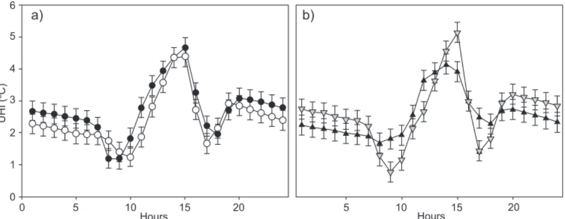
According to Stewart (2011), hourly observations are recommended for detection of the daily maximum and minimum UHI. When we examined the
variabil-ity of the UHIon hourly intervals (Fig. 10) we found
no interaction between the season effect (Fig. 10a) (P = 0.58, F = 0.30, 1, 235) and the canopy cover (Fig. 10b) (P = 0.47, F = 0.50, 1, 235). However,
significant differences through the hours were de
-tected (P ˂ 0.0001, F = 5.05, 23, 235). The UHI was
slightly more intense during warm nights and days according to Jáuregui (1997) and Romero-Dávila et al. (2011), who state that during the summer (warm) more and less urbanized zones receive high amounts of radiation, although they have different albedos.
Therefore, differences among Tmin were not
consid-erable. Nevertheless, during the night the response
to the slow rate of heat dissipation was significant in
more urbanized areas (Shahmohamadi et al., 2010). A pattern in UHI variation was detected inde-pendently of the season and status of the canopy
cover. During the first hours of the day (0:00 to
Fig. 10. Time hourly series for (a) urban heat island (UHI) intensity of monthly average minimum temperature (ΔTmin) throughout a day, during the cold (○) and warm (●) seasons described in
Fig. 4, and (b) low (▼–C) and high (▲+C) cover categories. Line bars are the standard errors
of the mean.
6
a) b)
5
4
3
UHI (ºC)
2
1
0
0 5 10
Hours 15 20 5 10 Hours 15 20
between more and less urbanized zones was mini-mal (Landsberg, 1981). Maximum UHI peaks were observed through the afternoon during the hours of highest solar radiation. This energy is absorbed and stored by the most urbanized surfaces, whereas less urbanized zones with greater percentages of
permeable surfaces (including vegetation) reflected
more radiation and therefore maintained smaller
superficial temperatures (Emmanuel, 2005; Blake
et al., 2011).
3.4 General considerations
The vegetation cover examined in the present work had a seasonal effect on air temperature and reduced the UHI intensity, although LAI peaks were relatively low (2.05 to 2.52), and vegetation types and their phenological activity were reduced because many species are deciduous during the cold season, and also as a result of the predominant summer rainfall distribution. In other studies a decrease in the UHI effect is reported, but the LAI is typically higher due to the temperate nature of vegetation and higher and more uniform rainfall regimes (Potchter et al., 2006; Leuzinger et al., 2010). Although the watering costs
may reduce the environmental benefits of urban veg -etation (Doick and Hutchings, 2013), here we have shown that vegetation types adapted to low rainfall are useful for reducing climate change effects. The cooling effect of urban vegetation, with likely higher water availability, was similar in magnitude to that of native species present in suburban areas and located at hill slopes. A further work should examine the
performance of native species under water-restricted regimes within the urban context.
The increase of green areas within the cities is an
efficient strategy to buffer environmental tempera -tures (Anyanwu and Kanu, 2006; Yu and Hien, 2006; Li et al., 2013). However, there are some drawbacks that should be considered when including trees in the urban landscape, such as litter production, infra-structure damage by roots, and emission of harmful volatile compounds (Anyanwu and Kanu, 2006; DEFRA, 2007; Doick and Hutchings, 2013). There-fore, careful selection of tree species and thorough planning are advised.
Urban parks are conspicuous and urban expansion is fast in Querétaro; therefore, a planned integration of adequate green areas is urgent. When increasing green land areas, sizeable areas should be considered
because their thermal influence depends on size (Jáu -regui, 1990; Ca et al., 1998; Yan et al., 2014). Even though the studied urban sites are small patches or household gardens, they still have an ameliorating effect. Besides the planning of big urban parks, empty lots could be reclaimed, which is important because some residential developments still have over 25% of unconstructed area after decades of being inaugurated.
4. Conclusions
More urbanized zones, higher temperature and a decreasing temperature gradient were associated to increasing vegetation cover. The effect of local climate zones could be associated to factors such as construction materials, infrastructure, extension of the impermeable surfaces, percentage of construction and fraction of permeable surface (vegetal cover and naked ground). Particularly, we demonstrated the im-portance of green areas, since a 50% increase in the
permeable surface diminished Tmin by 1.76 ºC during
the cold season and 2.18 ºC during the warm season. The UHI effect was similar regardless of the season (cold or warm), oscillating between 0.14 and 5 ºC. The UHI had a daily maximum of 4.2 ºC be-tween 13:00-16:00 LT, while a daily minima of the order of 1.5 ºC was nearly coincident with sunrise and sunset hours.
According to the relation showed by canopy cover and UHI intensity, a 50% increase in vegetation cover in urbanized zones could mitigate the UHI intensity up to 2.05 ºC during the warmest period.
Finally, it is important to emphasize that including green areas in urban planning is utterly important, since they have a potential for temperature mitigation. However, the design, extent and species composition of the canopy should take into account the existing urban climate and the species adaptation to climate variability.
Acknowledgments
This study was partially funded by Conacyt-Semar-nat (project 0108173), INE-UAQ (project INE/PS-051/2011), and Sedesu (Government of the State of Querétaro).
References
Adamson A., 2012. A textbook of physical chemistry, 2nd ed. Burlington Elsevier Science, 996 pp.
Alexander P. J. and G. Mills, 2014. Local climate
classi-fication and Dublin´s urban heat island. Atmosphere
5, 755-774.
Álvarez de la Torre G. B., 2010. El crecimiento urbano y estructura urbana en las ciudades mexicanas. Quivera
12, 94-114.
Anyanwu E. C. and I. Kanu, 2006. The role of urban forest in the protection of human environmental health in geographically prone unpredictable hostile weather conditions. Int. J. Environ. Sci. Te. 3, 197-201. http://www.sid.ir/en/VEWSSID/J_pdf/92220060213.pdf
Aragón-Domínguez M. E. and D. López-Carranza, 2013. La conformación de la Zona Metropolitana de Querétaro. Segundo Seminario Internacional Repensar la Metróp-oli. Mexico, 7-11 de octubre, 16 pp. Available at: http:// geouam.xoc.uam.mx/Seminario/PDFS/M12P3.pdf Baltazar J. O., M. Martínez y L. Hernández-Sandoval,
2004. Guía de plantas comunes del Parque
Nacio-nal “El Cimatario” y sus alrededores. Universidad
Autónoma de Querétaro, Mexico, 86 pp.
Blake R., A. Grimm, T. Ichinose, R. Horton, S. Gaffin,
S. Jiong, D. A. Bader and L. D. Cecil, 2011. Urban climate: Processes, trends, and projections. In: Climate change and cities: First assessment report of the Urban
Climate Change Research Network (C. Rosenzweig,
W. D. Solecki, S. A. Hammer, and S. Mehrotra, Eds.). Cambridge University Press, pp. 43-81.
Ca V. T., T. Asaeda and E. M. Abu, 1998. Reductions in air-conditioning energy caused by a nearby park.
Energ. Buildings 29, 83-92 pp.
CNA-SMN, 2014. Normales climatológicas. Base de datos climatológica para el estado de Querétaro a Julio de 2014. Available at: smn.conagua.gob.mx
DEFRA, 2007. Air quality and climate change: A UK perspective. Report of the Air Quality Expert Group to the UK Department of Environment, Food and Rural Affairs, 317 pp. Available at: http://uk-air.defra.gov.uk/ assets/documents/reports/aqeg/fullreport.pdf. Doick K. and T. Hutchings, 2013. Air temperature
regula-tion by urban trees and green infrastructure. Forestry Research, Forestry Commission, UK, 10 pp. Available
at: http://www.forestry.gov.uk/pdf/FCRN012.pdf/$file/
FCRN012.pdf.
Emmanuel M. R., 2005. An urban approach to cli-mate-sensitive design: Strategies for the tropics. Spon Press, Oxfordshire, 208 pp.
García-Cueto O. R., E. Jáuregui O., D Toudert and A. Tejeda, 2007. Detection of the urban heat island in Mexicali, B. C., Mexico and its relationship whit land use. Atmósfera 20, 111-131.
García-Cueto O. R., A. Tejeda Martínez y G. Bojórquez Morales, 2009. Urbanization effects upon the air temperature in Mexicali, B. C., México. Atmósfera
22, 349-365.
Guevara-Escobar A., M. Cervantes-Jiménez, H. Suzán-Az-piri, E. González-Sosa and I. Saavedra, 2012. Rhodes grass production under a Eucalypt canopy. Agrociencia
46, 175-188.
urban areas: Research dialogue in a policy framework.
Philos. Trans. R. Soc. A. 355, 2615-2629.
Icazuriaga-Montes C. y L. E. Osorio-Franco, 2007. La relación periferia-centro en la ciudad de Querétaro mediante las prácticas de movilidad y consumo. Al-teridades 17, 21-41.
INEGI, 1990. XI Censo General de Población y Vivienda
1990. Perfil sociodemográfico de Querétaro de Arteaga.
Instituto Nacional de Estadística y Geografía, Mexico. Available at: http://www.inegi.org.mx/sistemas/olap/ proyectos/bd/consulta.asp?p=16653&c=11893&s=est. INEGI, 2010. Principales resultados del Censo de Po-blación y Vivienda 2010: Querétaro. Instituto Nacional de Estadística y Geografía, Mexico, 84 pp. Available at: http://www.inegi.org.mx/prod_serv/contenidos/es- panol/bvinegi/productos/censos/poblacion/2010/prin-ci_result/qro/22_principales_resultados_cpv2010.pdf. IPCC, 1997. The regional impacts of Climate Change:
An assessment of vulnerability (R. T. Watson, M. C. Zinyowera and R. H. Moss, Eds.). Intergovernmental Panel on Climate Change, Cambridge University Press, 517 pp. Available at: http://www.ipcc.ch/ipccreports/ sres/regional/index.php?idp=0
IPCC, 2007. Cambio climático 2007. Informe de síntesis. Contribución de los grupos de trabajo I, II y III al Cuarto Informe de Evaluación del Grupo Interguber-namental de Expertos sobre el Cambio Climático (R. K. Pachauri y A. Reisinger, Dirs.). Geneva, 104 pp. Available at: http://www.ipcc.ch/pdf/assessment-re-port/ar4/syr/ar4_syr_sp.pdf
IPCC, 2013. Climate change 2013: The physical science basis. Contribution of Working Group I to the Fifth Assessment Report of the Intergovernmental Panel on Climate Change (T. F. Stocker, D. Qin, G.-K. Plat-tner, M. Tignor, S. K. Allen, J. Boschung, A. Nauels, Y. Xia, V. Bex and P. M. Midgley, Eds.). Cambridge University Press, Cambridge, United Kingdom and New York, 1535 pp. Available at: http://www.ipcc.ch/ report/ar5/wg1/.
Jáuregui E., 1990. Influence of a large urban park on
temperature and convective precipitation in a tropical city. Energ. Buildings 15, 457-463.
Jáuregui E., 1997. Heat island development in Mexico City. Atmos. Environ. 31, 3821-3831.
Jáuregui E., 2005. Possible impact of urbanization on the thermal climate of some large cities in México.
Atmósfera 18, 247-248.
Landsberg H. E., 1981. The urban climate. Academic Press, New York, 275 pp.
Leuzinger S., R. Vogt and C. Körner, 2010. Tree surface temperature in an urban environment. Agr. Forest Meteorol. 150, 56-62.
Li H., J. T. Harvey, T. J. Holland and M. Kayhanian, 2013.
Corrigendum: The use of reflective and permeable
pavements as a potential practice for heat island mit-igation and storm water management. Environ. Res. Lett. 8, doi:10.1088/1748-9326/8/1/01502314. Lin W., T. Wu, C. Zhang and T. Yu, 2011. Carbon savings
resulting from the cooling effect of green areas: a case study in Beijing. Environ. Pollut. 159, 2148-2154. Liu W., H. You and J. Dou, 2009. Urban-rural humidity
and temperature differences in the Beijing area. Theor. Appl. Climatol. 96, 201-207.
Lutgens F. K. and E. J. Tarbuck, 2012. The atmosphere: An introduction to meteorology, 12th ed. Pearsons, 533 pp. Mohanakumar K., 2008. Stratosphere-troposphere
inter-actions: An introduction. Springer, 416 pp.
Morillón G. D., F. R. Saldaña, T. I. Castañeda and M. U. Miranda, 2002. Atlas bioclimático de la República Mexicana. Energías Renovables y Medio Ambiente
10, 57-62.
Oke T. R., 1973. City size and the urban heat island. Atmos. Environ. 7, 769-779.
Oke T. R., 2006. Initial guidance to obtain representative meteorological observations at urban sites. Instru-ment and Observing Methods Report No. 81, WMO/ TD No. 1250. World Meteorological Organization, Geneva. Available at: http://www.urban-climate.org/ documents/IOM-81-UrbanMetObs.pdf.
Potchter O., P. Cohen and A. Bitan, 2006. Climatic be-haviour of various urban parks during hot and humid summer in the Mediterranean city of Tel Aviv, Israel.
Int. J. Climatol. 26, 695-711.
Romero-Dávila S., C. C. Morales-Méndez y X. A. Némiga,
2011. Identificación de las islas de calor de verano e
invierno en la ciudad de Toluca, México. Revista de Climatología 11, 1-10.
Shahmohamadi P., A. I. Che-Ani1, A. Ramly, K. N. A. Maulud and M. F. I. Mohd-Nor, 2010. Reducing urban heat island effects: A systematic review to achieve energy consumption balance. Int. J. Phys. Sci. 5, 626-636.
Stewart I. D., 2007. Landscape representation and the urban-rural dichotomy in empirical urban heat island literature, 1950-2006. Acta Climatologica et Choro-logica 40-41, 111-121.
Stewart I. D., 2011. A systematic review and scientific
critique of methodology in modern urban heat island literature. Int. J. Climatol. 31, 200-217.
Stewart I. D. and T. R. Oke, 2012. Local climate zones for urban temperature studies. Bull. Am. Meteorol. Soc. 93, 1897-1900.
Suzán-Azpiri H., V. H. Cambrón-Sandoval, O. R. García-Rubio, A.Guevara-Escobar, H. Luna-Soria y E. González-Sosa, 2014. Elementos técnicos del Programa Estatal de Acción ante el Cambio Climático-Querétaro. Universidad Autónoma de Querétaro, Mexico, 288 pp. Um H.-H., K.-J. Ha and S.-S. Lee, 2007. Evaluation of the urban effect of long-term relative humidity and the separation of temperature and water vapor effects. Int. J. Climatol. 27, 1531-1542.
United Nations, 2014. World urbanization prospects:
The 2014 revision, highlights. ST/ESA/SER.A/352.
United Nations, Department of Economic and So-cial Affairs, Population Division, New York, 32 pp.
Available at: http://esa.un.org/unpd/wup/Highlights/ WUP2014-Highlights.pdf
Wallace J. M. and P. V. Hobbs, 2006. Atmospheric science: An introductory survey, 2nd ed. Academic Press, El-sevier, 576 pp.
Wilby R. L., 2003. Past and projected trends in London’s urban heat island. Weather 58, 251-260.
WMO, 2008. Guide to meteorological instruments and methods of observation. Vol. I: Meteorology, 7th ed. WMO-No. 8. World Meteorological Organization, Geneva. 681 pp. Available at: http://www.wmo.int/ pages/prog/gcos/documents/gruanmanuals/CIMO/ CIMO_Guide-7th_Edition-2008.pdf
Yan H., S. Fan, C. Guo, J. Hu and L. Dong, 2014. Quantify-ing the impact of land cover composition on intra-urban air temperature variations at a mid-latitude city. PLoS ONE 9, doi:10.1371/journal.pone.0102124.
Yu C. and W. N. Hien, 2006. Thermal benefits of city parks.
Energ. Buildings Lausanne 38, 105-120.