Essays on education and economic performance

Texto completo

(1)Essays on Education and Economic Performance Laura Romero Valero. Supervisor: Dr. Carmen Beviá Baeza. Universitat Autònoma de Barcelona Departament d’Economia i d’Història Econòmica International Doctorate in Economic Analysis June 2003.

(2) A mis padres.

(3) Acknowledgements I would like to express my gratitude to those who have contributed with their help and support to the completion of this dissertation. First, I am deeply indebted to my supervisor, Carmen Beviá for her help and encouragement along the hard process of doing this thesis. I am also very grateful to Jordi Caballé who has followed my work as a second supervisor, and to Ignacio Conde, whose interest and support were crucial at the beginning of this project. The fourth chapter of this thesis is a joint work with Elena del Rey. I am really grateful for her collaboration in this work. This thesis has also benefited from comments and suggestions of Luis Corchón, Philippe De Donder, Íñigo Iturbe-Ormaetxe, Raquel Fernández, Omer Moav, Carmelo Rodríguez and Gilles Saint-Paul. My thanks to the Faculty and Students of IDEA for the friendly and cooperative research environment from which my research has greatly benefited. The support of my classmates and friends there: Debrah, Jana, Jernej, Jo, Julius, Kaniska, Maritxu, Nico, Óscar and Pablo, has been essential for me during these years. I really appreciate the hospitality of New York University, where I spent three unforgetable months as a visiting student. I am indebted to Raquel Fernández for her guidance and for all I have learnt from her. Special thanks to Anna and Luca, for their kindness and hospitality, and to Miquel, for his enthusiasm. This thesis has been completed during my stay at Université de Toulouse 1 as a Marie Curie visiting student. I am very grateful to Gilles Saint-Paul, who has followed my work during the academic year spent in Toulouse. I also thank Aude, for all her help, and Anna and Marta, for their friendship. Financial support from the Comissionat de Universitats i Recerca of Generalitat de Catalunya is also gratefully acknowledged. Finally, I want to express all my gratitude and love to my family, and especially to my parents, for being always so close even in the distance, and to Carmelo, for everything..

(4) Contents 1 Introduction. 1. Bibliography . . . . . . . . . . . . . . . . . . . . . . . . . . . . . . . . . . . . .. 7. 2 Education Subsidies, Income Inequality and Intergenerational Mobility. 9. 2.1 Introduction . . . . . . . . . . . . . . . . . . . . . . . . . . . . . . . . . . .. 9. 2.2 The Model . . . . . . . . . . . . . . . . . . . . . . . . . . . . . . . . . . . . 13 2.2.1. Production . . . . . . . . . . . . . . . . . . . . . . . . . . . . . . . 13. 2.2.2. Individuals . . . . . . . . . . . . . . . . . . . . . . . . . . . . . . . 14. 2.2.3. The Conditional Dynamical System . . . . . . . . . . . . . . . . . . 19. 2.2.4. Conditional Steady State Equilibria . . . . . . . . . . . . . . . . . 22. 2.3 Political Equilibrium . . . . . . . . . . . . . . . . . . . . . . . . . . . . . . 24 2.3.1. Preferred Subsidy Levels . . . . . . . . . . . . . . . . . . . . . . . . 24. 2.3.2. Majority Voting Equilibrium . . . . . . . . . . . . . . . . . . . . . . 29. 2.3.3. Equilibrium Subsidies and Inequality . . . . . . . . . . . . . . . . . 35. 2.4 The Evolution of the Economy . . . . . . . . . . . . . . . . . . . . . . . . . 38 2.4.1. Dynamics . . . . . . . . . . . . . . . . . . . . . . . . . . . . . . . . 38. 2.4.2. Steady State Analysis . . . . . . . . . . . . . . . . . . . . . . . . . 42. 2.5 Concluding Remarks . . . . . . . . . . . . . . . . . . . . . . . . . . . . . . 43 2.6 Appendix . . . . . . . . . . . . . . . . . . . . . . . . . . . . . . . . . . . . 45 Bibliography . . . . . . . . . . . . . . . . . . . . . . . . . . . . . . . . . . . . . 50.

(5) CONTENTS. iii. 3 Sorting into Public and Private Schools and Education Vouchers. 53. 3.1 Introduction . . . . . . . . . . . . . . . . . . . . . . . . . . . . . . . . . . . 53 3.2 The Model . . . . . . . . . . . . . . . . . . . . . . . . . . . . . . . . . . . . 57 3.2.1. Equilibrium under Perfect Capital Markets . . . . . . . . . . . . . . 59. 3.2.2. Equilibrium under Borrowing Constraints . . . . . . . . . . . . . . 62. 3.3 Analysis of Education Vouchers . . . . . . . . . . . . . . . . . . . . . . . . 65 3.3.1. Equilibrium with Education Vouchers . . . . . . . . . . . . . . . . . 66. 3.3.2. Political Economy of Education Vouchers . . . . . . . . . . . . . . . 70. 3.4 Calibration and Illustrative Results . . . . . . . . . . . . . . . . . . . . . . 79 3.4.1. Benchmark Economy . . . . . . . . . . . . . . . . . . . . . . . . . . 79. 3.4.2. Introduction of Education Vouchers . . . . . . . . . . . . . . . . . . 81. 3.5 Concluding Remarks . . . . . . . . . . . . . . . . . . . . . . . . . . . . . . 84 Bibliography . . . . . . . . . . . . . . . . . . . . . . . . . . . . . . . . . . . . . 86 4 Competition between Public and Private Universities: Exams versus Prices. 88. 4.1 Introduction . . . . . . . . . . . . . . . . . . . . . . . . . . . . . . . . . . . 88 4.2 The Model . . . . . . . . . . . . . . . . . . . . . . . . . . . . . . . . . . . . 92 4.2.1. Individuals . . . . . . . . . . . . . . . . . . . . . . . . . . . . . . . 92. 4.2.2. Universities . . . . . . . . . . . . . . . . . . . . . . . . . . . . . . . 93. 4.2.3. Allocation Mechanisms . . . . . . . . . . . . . . . . . . . . . . . . . 93. 4.3 The monopoly benchmark . . . . . . . . . . . . . . . . . . . . . . . . . . . 94 4.3.1. Perfect Capital Markets . . . . . . . . . . . . . . . . . . . . . . . . 95. 4.3.2. Borrowing Constraints . . . . . . . . . . . . . . . . . . . . . . . . . 99. 4.4 Competition between a Public and a Private University . . . . . . . . . . . 104 4.4.1. Equilibrium under Perfect Capital markets . . . . . . . . . . . . . . 104. 4.4.2. Equilibrium under Borrowing Constraints . . . . . . . . . . . . . . 109. 4.5 Concluding Remarks . . . . . . . . . . . . . . . . . . . . . . . . . . . . . . 113.

(6) CONTENTS. iv. 4.6 Appendix . . . . . . . . . . . . . . . . . . . . . . . . . . . . . . . . . . . . 114 Bibliography . . . . . . . . . . . . . . . . . . . . . . . . . . . . . . . . . . . . . 124.

(7) Chapter 1 Introduction Economists have devoted considerable attention to understanding the role of human capital on economic performance. This is not surprising given the enormous relevance of human capital to economic well being. The underlying notion behind the concept of human capital is that individuals make investment decisions in education that allows them to acquire the skills that are relevant for the labor market. The accumulated skills resulting from these investments represent the human capital of an individual. The empirical work on human capital has concentrated mainly on the impact of educational attainment or years of schooling on economic growth. This literature documents the existence of a positive correlation between educational attainment, especially primary education, and the average growth rate of countries.1 Theoretical contributions to understanding the fundamental role of human capital on economic development date back to Lucas (1988), who attribute the differences in growth rates among countries to the disparities in the rates at which countries accumulate human capital over time. In analyzing human capital and its implications for future outcomes, it has been frequently ignored where individuals’ skills come from or how human capital is produced. Economic research on the determinants of education and its consequences has only recently 1. See for instance Mankiw et al (1992), Benhabib and Spiegel (1994) and Barro and Sala-i-Martin. (1995)..

(8) 2 attracted the interest of researchers. Formal schooling, individual abilities, family income and cultural background are some of the factors that contribute to the accumulation of human capital. Cognitive skills, measured by students’ performance on standardized tests, are found to be positively related to individual earnings, productivity and economic growth. The earnings advantages to higher scores on standardized tests, after holding constant years of schooling, are documented in a number of empirical studies.2 Family background and, in particular, the level of education of the parents is also a crucial factor in determining the educational attainment of the children. There is evidence supporting the fact that the probability of attending college is higher for the children of parents with university degrees. For instance, adults of educated parents are between three and four times more likely to attain tertiary education than those with uneducated parents (see OECD (1998)). Investments in education take two forms: direct investments of the parent’s time and investments in formal schooling that must be purchased in the market. The skills of parents in educating the child, and hence, the quality of the time devoted to his education, seem to be influenced by parental educational attainment. Investments in formal education return future economic benefits in the same way as a firm investing in physical capital returns future production and income. These investments are guided first, by their expected return, which is estimated to be high: between 17 and 22 percent for lower education, 15 and 16 percent for high school, 12 and 13 percent for college and 7 percent for graduate school (Willis, 1986). The second factor affecting investment decisions in education is parental resources. The evidence is strong that family income has an important effect on the probability of staying in school, at every level of education.3 The unobservability of children’s ability, moral hazard problems and the fact that de2. The earnings advantages to higher performance is documented in Bishop (1989), Grogger and Eide. (1993) and Neal and Johnson (1996). On the other hand, Hanushek and Pace (1995) find that college completion is significantly related to higher test scores at the end of high school. 3 See Cameron and Heckman (1996)..

(9) 3 cisions are made by parents on behalf of their children suggest that education is a special investment good. Moreover, the inability of parents to borrow against the future human capital of their children leads to inefficient educational investments by low income families. Thus, a system where parents finance the education of their children is inefficient. Since investments in human capital depend on parental income, and income vary across parents, educational attainment will vary across children for reasons unrelated to children’s characteristics, such as their cognitive abilities. The importance of the acquisition of skills appears in its effects on the earnings of individuals and on the subsequent distribution of income in the economy. Thus, if differences in parental resources affect the future earnings of children, the inequality associated to social immobility in the earnings distribution will persist over time. As long as the marginal return from investing in education is greater for high-ability students, high persistency in economic status suggests that there is substantial underinvestment at the bottom of the income distribution. Hence, improvements in the quality of education for children from poor families will increase efficiency, since a higher correlation between children’s cognitive skills and investments in education raises the accumulation of human capital. The inexistence of a market for loans to finance educational investments, especially in primary and secondary education, may help explain why in all countries governments subsidize education. If one of the objectives of the government is to ensure equal opportunity, the subsidization of education may correct inefficiencies in the capital markets allowing low income students to have access to education at almost no cost. However, government intervention in education is not restricted to subsidize a certain amount of education. In most countries, education -even at the tertiary level- is publicly provided, although these educational services are available in the private market. This public provision may be rationalized on the basis of the external effects of education, especially at the primary and secondary levels. Thus, the government provides citizens with a minimum degree of literacy that benefits the society as a whole..

(10) 4 Another argument that regards education as a special good is that each student creates externalities for other students and for the educational process. The quality of the education any student obtains from school or college depends in good measure on the quality of that student’s peers. Along with per-student expenditures and school’s facilities, average scores on standardized tests are often used as a measure of institutional quality. The special features of the educational production make the market for education different from other markets. The customers in this market, the students, are also the input in the production of school quality. Educational institutions are publicly owned in many countries, but frequently face competition from private institutions. Some private educational institutions pursue profits while others have different goals. This dissertation consists of three chapters exploring different aspects of education and its effects on economic performance. Chapter 2 and Chapter 3 investigate the effects of public subsidization of education on human capital accumulation and income distribution. In these chapters, I adopt the approach of modelling public education policies as the equilibrium outcome of a political process. This approach differs from policy analysis in the traditional Public Finance, which is almost entirely normative, and it instead focuses on positive issues, combining economic and political analysis. Chapter 4 analyzes the strategic interaction among educational institutions in the higher education market. The approach taken in this chapter builds on industrial organization models of competition. The study of intergenerational mobility, that is, the correlation of economic or education status among individuals belonging to the same family, is important for economic performance. Mobility implies a higher correlation between the ability of individuals and their educational attainment and thus, since high-ability individuals obtain a higher return to educational investments, economic resources are more efficiently allocated in mobile economies. Chapter 2 investigates on the one hand, the impact of education subsidies on intergenerational mobility and on the other, the conditions under which the subsidization of education emerges as a political equilibrium. In the absence of capital.

(11) 5 markets to finance investments in human capital, education subsidies play a key role in intergenerational mobility. We find that the political support of these subsidies depends positively on the level of development of the economy, which is measured by the proportion of educated individuals. Interestingly, the impact of income inequality on the size of the subsidy is not monotone. In our model, income inequality raises with the wage gap between educated and uneducated labor. Intuitively, a low wage gap reduces incentives to invest in education while a high level of inequality raises the conflict of interests among poor and rich individuals over the degree of subsidization of education. Hence, we obtain that the magnitude of the subsidy is higher at intermediate levels of inequality. Government intervention in education frequently takes the form of public provision. Advocates of school choice argue that a public school system offering a uniform -and frequently low- educational quality, independently of individuals’ specific needs may fail to ensure equal educational opportunities. Discontent with public schools in many countries may help explain the interest on issues related to school choice, including education vouchers. A voucher program provides students attending private schools a tax-financed payment covering all or most of the tuition charged. Chapter 3 evaluates the impact of education vouchers on the efficient sorting of students into public and private schools. Private schools offer a continuum of quality levels, while public schools provide a uniform quality, funded with proportional taxes. Students differ over family income and ability and parents choose between public and private schools. We find that a tax-minimizing voucher will be approved by majority when the level of public educational quality is sufficiently high. In the calibrated model, the equilibrium voucher entails welfare gains although leads to greater inequality. The impact of different voucher policies is also analyzed. We find that welfare gains increase with the voucher size but the impact of the magnitude of the voucher on income inequality is not monotone. The provision of education, in contrast to other goods, is not allocated only by prices. Higher education institutions usually use exams to allocate students to schools. The.

(12) 6 importance of this instrument varies depending on the country and institution. In many European countries, public universities set very low prices and use exams as the main guide to determine their admissions while private universities are usually of lower quality. In contrast, in the United States the majority of universities are private and non-profit institutions and both exams and prices play an important role as instruments to allocate students. Chapter 4 focuses on optimal choices of prices and exams by universities in the presence of borrowing constraints. There are two institutions, one public and one private, providing educational quality in the higher education market. Students differ in their unobservable ability and in their income endowment and they choose whether to attend a university or remain uneducated. We first compare the optimal behavior of a public monopoly, maximizing public surplus, with the optimal choices of a private monopoly, maximizing profits. We find that the private university only uses prices as allocation device, while the public institution uses exams while setting a zero price for its educational services in the presence of borrowing constraints. Next, we model competition between a public and a private university and we show that in equilibrium, the public university provides a higher quality than the one provided privately. This result may be explained by the different strategies, exams versus prices, followed by the public and the private university respectively. The use of exams allows the public university to behave as a monopoly in the higher education market and the private university attracts those students of lower ability who are not accepted at the public institution..

(13) BIBLIOGRAPHY. 7. Bibliography [1] Barro, R.J. and Sala-i-Martin, X. (1995). Economic Growth, New York: McGrawhill. [2] Benhabib, J. and Spiegel, M.M. (1994), “The Role of Human Capital on Economic Development: Evidence from Aggregate Cross-Country Data”. Journal of Monetary Economics 34 (2): 143-173. [3] Bishop, J. (1989), “Is the Test Score Decline Responsible for the Productivity Growth Decline?”. American Economic Review 79, No. 1: 178-197. [4] Cameron, S.V. and Heckman, J.J. (1996), “Life Cycle Schooling and Educational Selectivity: Models and Evidence”. Manuscript, University of Chicago. [5] Grogger, J.T. and Eide, E. (1993), “Changes in College Skills and the Rise in the College Wage Premium”. Journal of Human Resources 30, No. 2: 280-310. [6] Hanushek, E.A. and Pace, R.P. (1995), “Who Teaches to Teach (and Why)?”. Economics of Education Review 14, No. 2:101-117. [7] Hanushek, E.A. (2002), “The Importance of School Quality”. Manuscript, Hoover Institution, Stanford University. [8] Lucas, R.E., Jr. (1988), “On the Mechanics of Economic Development”. Journal of Monetary Economics 22: 407-437. [9] Mankiw, N.G., Romer, D. and Weil, D.N. (1992), “A Contribution to the Empirics of Economic Growth”. Quarterly Journal of Economics 107 (2): 407-437. [10] Neal, D.A. and Johnson, W.R. (1996), “The Role of Pre-Market Factors in BlackWhite Differences”. Journal of Political Economy 104, No. 5: 869-895. [11] OECD (1998), “Education at a Glance”. Centre for Educational Research and Innovation, Paris..

(14) BIBLIOGRAPHY. 8. [12] Willis, R.J. (1986), “Wage Determinants: A Survey and Reinterpretation of Human Capital Earnings Functions”. In Orley Ashenfelter and Richard Layard, eds., Handbook of Labor Economics, Vol. I. Amsterdam: North Holland..

(15) Chapter 2 Education Subsidies, Income Inequality and Intergenerational Mobility 2.1. Introduction. In any society, individuals are born with different parental income, learning ability and family background. We may claim that society provides equal opportunity to its members when individuals’ future success is largely unpredictable on the basis of family background. Consequently, we can judge if there is equal opportunity by looking at parents and their children to evaluate whether children’ success is determined in large part by their parents’ income. In the presence of imperfect capital markets to finance the acquisition of human capital, parental income becomes a crucial factor in determining future children’ economic status.1 Thus, since rich families tend to invest more in their children’ education, we expect that initial differences in income across parents will affect their offspring’s economic 1. For instance, it is well documented that children from rich families are more likely to attend university. than children from poor families..

(16) 2.1 Introduction. 10. success. A high persistence in economic status across generations within the same family is therefore, an indicator of low intergenerational mobility. The study of mobility is also important for human capital accumulation, since mobility implies a higher correlation between individual’s ability or effort, and educational attainment. As long as the marginal return from studying is greater for talented students, a higher intergenerational mobility means that resources are allocated more efficiently and thus, the accumulation of human capital raises. Moreover, there exists some empirical evidence that mobility is positively correlated with income equality and that it is higher in more developed economies.2 This chapter investigates the impact of education subsidies on intergenerational mobility and analyzes the conditions under which the subsidization of education emerges as a political equilibrium. The novel feature of this work is precisely the endogenous determination of this education policy in a dynamic context.3 The initial income distribution plays a crucial role in the evolution of the economy because it determines the equilibrium level of subsidization of education and thus, the proportion of individuals investing in education. Thus, economies with different levels of income per capita and inequality choose different levels of education subsidies and exhibit very different patterns of mobility. Our work is related to two different lines of research: the literature on income inequality and redistributive politics and the line of research studying the relationship between income inequality and intergenerational mobility. The first strand of literature links income inequality and economic development through the effect that income distribution has on redistribution, and its subsequent effects on economic growth. In this literature, 2. Becker and Tomes (1986) survey a number of empirical studies for different countries showing a. positive relationship between intergenerational mobility and income per capita. Björklund and Jäntti (1997) show that Sweden has higher income equality and intergenerational mobility than United States. Contradictory findings appear in Checchi et al. (1999) who show that Italy is more equal but less mobile than the US. 3 Fernández and Rogerson (1995) have investigated the endogenous determination of education subsidies in a political process but their model is static..

(17) 2.1 Introduction. 11. we can distinguish two different approaches explaining the negative relationship between income inequality and economic growth supported by some data. In the approach of Persson and Tabellini (1994) and Alesina and Rodrik (1994) growth accrues from the accumulation of physical capital. Thus, the link between initial income inequality and subsequent growth is the higher taxation on investment induced by higher inequality, which is translated into a poorer median voter who pressures for more redistribution. This, in turn discourages investment and growth. Another explanation for the negative relationship between income inequality and growth comes from the theoretical literature on human capital accumulation in the presence of credit market imperfections. According to this literature, it is the existence of decreasing returns in the accumulation of this production factor which makes redistribution toward those individuals with lower human capital endowments to increase growth. However, empirical evidence is not conclusive about the relationship between income inequality and economic development and some theoretical papers provide an explanation for these contradictory empirical findings. For instance, Perotti (1993) shows that the level of development is crucial in determining the effects that both the level of income inequality and the equilibrium level of taxation may have on economic growth. In SaintPaul and Verdier (1993), higher inequality leads to higher growth because it induces a higher expenditure in public education, which is the source of growth in their model. In the second strand of literature, Becker and Tomes (1986) and Loury (1981) analyze the dynamic relationship between income inequality and intergenerational mobility under imperfect capital markets, in the context of an unchanging macroeconomic environment, in which mobility does not affect the return of education. Owen and Weil (1998) investigate the interaction between economic growth and intergenerational mobility with a model that allows them to compare the degree of mobility between economies that are at different stages of the development process. While their analysis is restricted to steady state equilibria, Maoz and Moav (1999) study the dynamics of inequality and mobility along.

(18) 2.1 Introduction. 12. the growth path. In both papers, the existence of complementarities between educated and uneducated labor provides a theoretical explanation, in the context of a changing economic environment, for the positive relationship between economic development, mobility and income equality supported by some empirical literature. This work merges these two lines of research to investigate the connection between income inequality, intergenerational mobility and endogenous education policies. We present an overlapping-generations model based in Maoz and Moav (1999), in which individuals are heterogenous in their parents’ income and in their innate ability to learn. Capital markets are inexistent and thus, investments in human capital depend crucially on parental income and the size of education subsidies. In our model, human capital accumulation accrues from an increase in the proportion of individuals who invest in education over time. This process is fueled by intergenerational mobility of individuals born of uneducated parents who acquire education. The equilibrium degree of subsidization of education is the outcome of a political process. The level of education subsidies is chosen by majority voting by individuals with conflicting interests regarding the education policy. This conflict reflects socio-economic factors derived from differences across them, either in terms of income or ability, and these factors are those shaping the distribution of individuals’ preferences over the magnitude of subsidization of education. Education subsidies finance partially the cost of acquiring education, which depends negatively on individuals’ ability, and they are funded by proportional taxes over total income in the economy. Education subsidies are available only to those individuals who acquire education.4 In our model, mobility raises when the size of the subsidy is sufficiently high to allow some individuals from poor families to invest in education. In this case, education subsidies become an endogenous mechanism to generate mobility in economies stuck in 4. In developed economies, education subsidies are intended to partially finance the costs of acquiring. tertiary education, since primary and secondary education are completely funded publicly. However, in poor countries, they may subsidize lower education levels..

(19) 2.2 The Model. 13. poverty traps. We find that a minimum level of development, measured by the proportion of educated individuals in the economy, is required for the political support of education subsidies. This result may be explained by the inexistence of a capital market to finance the acquisition of education. Thus, in poor economies the proportion of individuals acquiring education is low and education subsidies cannot be supported by a majority of individuals in the economy. The level of income inequality is also a relevant variable in determining the equilibrium degree of subsidization of education. We obtain that the magnitude of the subsidy is higher at intermediate levels of income inequality. In our model, income inequality is monotone in the wage gap between educated and uneducated labor. Intuitively, a low wage gap reduces incentives to invest in education while a high level of inequality raises the conflict of interests among poor and rich individuals over the degree of subsidization of education. In both cases, the political support of this education policy decreases. This chapter is structured as follows. Section 2.2 presents the economic environment in which individuals’ economic decisions and the conditional evolution of the economy are analyzed. In Section 2.3 the political equilibrium level of education subsidies is characterized. Section 2.4 studies the effect of endogenous education subsidies in the process of development, and how both the dynamics and the steady state level of educated individuals are affected by such subsidies. Finally, in section 2.5 we present some concluding remarks.. 2.2. The Model. 2.2.1. Production. The economy produces a single homogeneous good that can be devoted to either consumption or investment in education. Aggregate output is given by a linear production.

(20) 2.2 The Model. 14. function of educated labor Et , and uneducated labor Ut , in period t : Yt = wE Et + wU Ut ,. (2.1). where wE and wU are the wages or marginal productivity of educated and uneducated labor respectively. We assume that educated individuals are more productive than uneducated individuals and the wage of educated labor is at least as twice the wage of uneducated labor, wE ≥ 2 wU .5 We choose this simple production function in order to analyze the role of education subsidies in the degree of intergenerational mobility of the economy. For instance, with a Cobb-Douglas production function in which both labor types are complements, intergenerational mobility would be affected by labor wages and thus, it would be difficult to isolate the role of education subsidies in mobility. Individuals supply inelastically one unit of labor, either as educated or uneducated. The total number of individuals in the economy is normalized to one and is equal to the number of individuals living in each generation. Thus, we can express the proportion of uneducated workers, Ut = 1 − Et as a function of Et .. 2.2.2. Individuals. We consider an overlapping generations economy, in which individuals live for two periods. Each individual gives birth to another in his second period of life, so population remains constant over time and is normalized to one. In their first period of life, young individuals do not work. They receive a transfer from their parents that may be used either to consume or to purchase education. Young individuals also decide by majority voting the level of education subsidies in this period.6 In their second period of life, individuals work 5. The wage ratio of educated labor to uneducated labor is usually measured by the 90th-10th percentile. of the wage distribution and this ratio is above 2 in OECD countries. See Machin (2002). 6 It would be equivalent, in terms of preferred subsidies of individuals, to consider that it is the old generation the one who is choosing the subsidization of education of their children..

(21) 2.2 The Model. 15. as either educated or uneducated laborers. They do not consume in this period since they bequeath all their labor income to their offsprings. Young individuals differ not only in the bequest received from their parents, but also in their innate ability. Differences in abilities are represented by different education costs.7 The ability of a young individual i is independent of both the ability and income of his parent and it is inversely correlated with his education cost, hi . Education costs are £ ¤ uniformly distributed in the interval h, h , where h > 0.8. We assume that capital markets to finance investments in education are inexistent, and. thus, young individuals cannot borrow against their future income to acquire education. This assumption implies that individuals’ wealth in their second period of life is only their labor income. Since education is costly and borrowing is not possible, some individuals may not be able to afford an education, or they may not be willing to acquire it in order to increase first-period consumption. Individuals derive utility from consumption in their first period of life and from transfers to their children when they are old. Old individuals obtain utility from the size of the bequest they leave to their offsprings. Therefore, altruism of the parents is based on the “joy of giving” motive.9 The utility function is logarithmic and equal for all individuals born in period t: i i Uti (cit , wt+1 ) = ln cit + ln wt+1 ,. (2.2). i where cit is the consumption of individual i when he is young, in period t and wt+1 is the. bequest he passes to his child when he is old, in period t + 1. The utility maximization problem of a young individual can be solved backwards in two stages. In the first stage, he chooses his most preferred subsidy and the equilibrium level of education subsidies is decided by majority voting. Only those individuals who 7. Education costs summarize both monetary and opportunity costs of purchasing education. Such. opportunity costs represent lost consumption in the first period. 8 If h = 0, the acquisition of education does not involve any cost for some high-ability individuals. 9 This type of altruism also appears in Galor and Zeira (1993) and Banerjee and Newman (1993)..

(22) 2.2 The Model. 16. acquire education in period t are eligible to receive education subsidies, St . These subsidies are funded by proportional taxes θt over bequests or total first-period income, wt , which is the average wage in period t wt = Et wE + (1 − Et ) wU = Yt .. (2.3). In the second stage, individuals decide whether to acquire education or not, given the level of education subsidies, St and the proportional tax rate over total income, θt . We first solve this stage of young individuals’ utility maximization problem and we leave the analysis of political decisions for the next section. In our economy, individuals only make economic decisions in their first period of life, when they decide whether they purchase education or not, since in the second period they i just bequeath their labor income, wt+1 to their offsprings. Since there are no savings, the. only way for a young individual to increase his future income is by means of investing in education. The decision of acquiring education varies across young individuals, since they i , i = E, U and in their education differ in the transfer received from their parents, wt+1 ¤ £ costs, hi ∈ h, h .. Old individuals belonging to the same type, either educated or uneducated, receive. the same wage, and thus, there are only two levels of second-period income and hence, of bequests. Thus, the superindex i corresponding to the transfer a young individual receives from his parent can be replaced by his parent’s type: E or U. Labor wages for educated i = wi , i = E, U. and uneducated labor are constant over time and thus, wti = wt+1. A young individual i must substitute first-period consumption for second-period income to acquire education, since he has to give up consumption in order to become educated.10 Thus, an individual i investing in education consumes cit = (1 − θt )wi + St − hi in his first period of life and earns the educated labor wage, wE in the second period. Conversely, if he decides not to become educated, he instead consumes, cit = (1 − θt )wi 10. Note that those individuals with education costs below the level of subsidies, hi < St are able to. purchase education without giving out first period consumption..

(23) 2.2 The Model. 17. and obtains the uneducated labor wage, wU in the second period of his life. Hence, a young individual i will invest in education if and only if the indirect utility derived from purchasing education, UtE is higher or equal than the utility derived from not investing in human capital, UtU : UtE ≥ UtU ,. (2.4). where UtE = ln((1 − θt )wi + St − hi ) + ln wE and UtU = ln ((1 − θt )wi ) + ln wU . Condition (2.4) may be interpreted as follows: given the transfer received from his father, wi , the level education subsidies, St and the tax rate, θt , an individual i will invest in education if and only if his education cost, hi is small enough. This condition hit , such that only those individuals with an education determines a critical education cost, b hit acquire education: cost below this threshold, hi ≤ b µ ¶ U ¡ ¢ w i i b ht = (1 − θt )w 1 − E + St ≡ b hi wE , wU , θt , St . w. (2.5). hit is a continuous and differentiable function of all their components, we obtain Since b. the following derivative signs:. ∂b hit ∂b hit ∂b hit ∂b hit ´ ³ > 0, < 0, > 0. > 0, U ∂wi ∂θt ∂St ∂ 1− w E w. (2.6). The first of the above derivatives shows how a higher bequest, wi increases the probability that a young individual invests in education. The second derivative means that a higher wage gap between educated and uneducated labor serves as an incentive for purchasing education.11 A higher tax rate affects negatively the threshold cost, since it hit with reduces first-period disposable income and the positive sign of the derivative of b 11. Note that an increase in the wage of uneducated labor, wU has two effects of opposite sign on the. U critical cost of individuals born of uneducated parents, b hU t . On the one hand, an increase in w relaxes. constraints to invest in education for these individuals and on the other, it decreases the wage ratio of. educated to uneducated labor and therefore, the incentives to acquire education are lower. Note that the net effect is positive, i.e.,. ∂b hU t ∂wU. ≥ 0 since. wE wU. ≥ 2..

(24) 2.2 The Model. 18. respect to the education subsidy shows how this subsidy reduces the cost of acquiring education. Since there are only two income types, either educated or uneducated, we have two critical values for education costs ³ E b hE 1− = (1 − θ )w t t ³ b hUt = (1 − θt )wU 1 −. wU wE. ´. ´ U. w wE. + St ,. (2.7). + St ,. bU hE where b t and ht are the critical cost levels for young individuals born of educated and. uneducated parents respectively.. Note that old educated individuals earn more and thus, they bequeath more than uneducated individuals, and this makes the critical cost of education for their children higher or equal than the critical cost of those of uneducated parents, b bU hE t ≥ ht , ∀θ t ∈ [0, 1] .. (2.8). From (2.8) it follows that there exists a positive correlation between educational attainment of the children and the level of education of the parents since the child of an educated parent is more likely to acquire education than the child of an uneducated parent.12 We assume throughout the paper that the following condition holds: wE − wU > h.. (A1). Assumption (A1) implies that in the absence of education subsidies, some individuals born of educated parents always acquire education since their critical cost is strictly higher hE than the minimum cost of education, b t > h. Thus, the wage gap between educated and uneducated labor, wE − wU must be strictly higher than the minimum cost of education,. h for some individuals born of educated parents to be willing to invest in education. 12. This result is a direct consequence of the inexistence of capital markets in the economy and it does. not require the child’s ability to be correlated with the parent’s education or ability..

(25) 2.2 The Model. 2.2.3. 19. The Conditional Dynamical System. We now turn to study the evolution of the economy, conditional on the level of education subsidies.13 The economy grows when the proportion of individuals who purchase education raises over time as the result of dynasties’ mobility from one labor type to the other. Upward mobility takes place when some individuals born of uneducated parents purchase education and equivalently, downward mobility occurs when some individuals born of educated parents do not to invest in human capital. Thus, an increase in the number of educated individuals, Et takes place when the number of upward-mobile individuals, (1 − Et )F (b hUt ) exceeds the number of downward-mobile individuals, Et (1 − F (b hE t )).. The proportion of individuals purchasing education in period t and working as edu-. cated labor in period t + 1, Et+1 is simultaneously determined by the following equations: bU hE Et+1 = Et F (b t ) + (1 − Et )F (ht ),   θt wt if Et+1 > 0, Et+1 St =  0 if E = 0.. (2.9) (2.10). t+1. It follows from (2.9) that the number of individuals who acquire education in period t, Et+1 is the sum of individuals of educated parents, Et F (b hE t ) and individuals of un-. hUt ) who invest in education in this period, where b hE educated parents, (1 − Et )F (b t = ¡ ¢ ¡ ¢ b hE wE , wU , St , θt and b hE wE , wU , St , θt are given by (2.7) . hUt = b. The proportion of individuals who invest in education in period t is also determined. by the level of per-student subsidies in period t, St , which consists of total government revenues, θt wt divided by the number of individuals purchasing education in period t, Et+1 . Solving equation (2.10) for θt and substituting into (2.9), we obtain Et+1 as an implicit 13. In this section, we consider that the level of subsidies is exogenously given and constant over time. and hence, the tax rate varies over time as the economy evolves. The dynamic analysis performed in this section is conditional on a given level of education subsidies..

(26) 2.2 The Model. 20. function of Et and St : Et+1 = Et F (b hE (Et , Et+1 , St )) + (1 − Et )F (b hU (Et , Et+1 , St )).. (2.11). In every period t, the conditional evolution of the economy is completely characterized by the proportion of educated individuals, Et , since education subsidies are exogenous and constant over time, St = S ∈ [0, Stmax ] .14 The following proposition states that Et+1 is uniquely determined by Et . Proposition 2.1. In the range 0 < Et < 1 there exists a unique Et+1 ∈ (0, 1] , which is the solution to (2.11) for any Et . Proof. First, we prove that Et+1 > 0, ∀Et ∈ (0, 1). Assume that Et+1 = 0, then S = 0. hE and under (A1), b t > h, which implies that the right-hand side of (2.11) is strictly positive. and thus, it contradicts Et+1 = 0.. Existence of a unique Et+1 ∈ (0, 1] holds since the right-hand side of (2.11) is a continuous and strictly decreasing function of Et+1 from (2.7) and (2.10), while the left-hand side is increasing in Et+1 with a slope of one. We assume that the initial proportion of individuals in the economy is strictly positive, 0 < E0 < 1, and thus, from Proposition 2.1 at any period t the number of educated individuals is strictly positive. The following proposition shows that, given the level of the subsidy S, in economies with mobility an increase in the magnitude of subsidization of education raises the number of individuals acquiring education. Proposition 2.2. In economies with mobility, an increase in the level of education subsidies raises the number of individuals who invest in education. Proof. In economies with mobility, there exists either downward mobility or upward mobility, or both. We define the following function: ¢ ¢ ¡ ¡ G (Et , Et+1 ) = Et+1 − Et F (b hE Et , Et+1 , S ) − (1 − Et )F (b hU Et , Et+1 , S ).. 14. bE bU Note that the law of motion of the economy is stable since F (b hE t ) ≤ 1 and F (ht ) ≥ F (ht )..

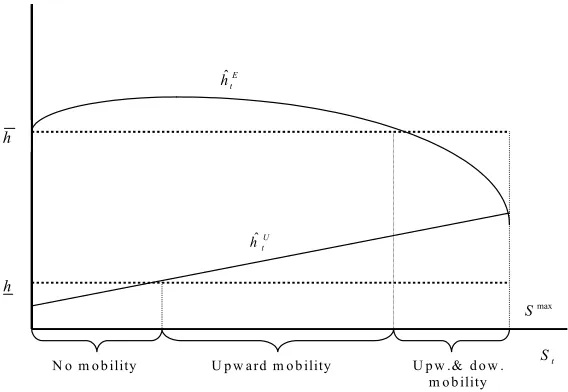
(27) 2.2 The Model. 21. We apply the implicit function theorem to compute the effect of an increase in the level of education subsidies, S on the proportion of individuals acquiring education, i.e.,. ∂Et+1 . ∂S. This theorem holds since G is a continuous function of Et , Et+1 and S and as follows from ) = 0. Proposition 2.1, there exists a unique Et+1 for each Et , such that G (E³t , Et+1 ´ ∂Et+1 ∂S. From (2.7) , we find that ´ ³ U < 1 and Et+1 ≤ 1 and 1 − w E w. =. ∂G ∂Et+1. − ∂G. ∂S ∂G ∂Et+1. U. > 0, where. > 0 since. ∂F (b hi ) ∂Et+1. ∂G ∂S. =. −1+Et+1 1− wE w. h−h. < 0, since. < 0, i = E, U.. An increase in education subsidies raises upward mobility, since it allows more individuals born of uneducated parents to acquire education and the redistributional role of subsidies makes poor families to benefit more from an increase in the level of subsidies than rich families.15 It is also of interest to understand which is the role of education subsidies in economies without mobility. These economies are characterized by a perfect correlation between young individuals’ educational attainment and parental education or income. Hence, the probability that an individual born of a educated parent chooses to acquire education hE is equal to one, F (b t ) = 1 and conversely, the probability that an individual with an. hUt ) = 0. Figure 2.1 shows the uneducated parent invests in education is equal to zero, F (b bU hE effects of education subsidies on critical values, b t and ht . For low levels of the subsidy,. bU hE there is no mobility since b t ≥ h and ht < h. Upward mobility occurs when the subsidy hUt is sufficiently high and the critical cost of individuals born of uneducated parents, b. hUt > h. In this case, the subsidy raises crosses the lower limit of the cost distribution, b. disposable income of poor families in an amount high enough to allow some children of. uneducated parents to acquire education. Similarly, downward mobility exists when the critical value of the cost of education for young individuals with educated parents crosses hE the upper limit of the cost distribution, b t < h. This situation happens when the subsidy reduces disposable income of rich families and some individuals born of educated parents 15. Downward mobility raises only if the subsidy is sufficiently high to reduce disposable income of rich. families..

(28) 2.2 The Model. 22. do not invest in human capital as Figure 2.1 illustrates.. ĥ tE. h. hˆ tU. h S max. N o m o b ility. U p w a rd m o b ility. U p w .& d o w . m o b ility. St. bU hE Figure 2.1: Effect of St on critical levels, b t and ht .. 2.2.4. Conditional Steady State Equilibria. A conditional steady state equilibrium is defined as the proportion of educated individuals, E ss that is invariant over time when the education subsidy is constant and exogenously given. Steady state equilibria can be characterized by the existence of intergenerational mobility of dynasties, from an education type to the other, or by no mobility. The possible laws of motion of the economy are the following:16 bU hE 1. Only downward mobility: h < b t < h and ht < h for all t > 0.. In such an economy, only some individuals with educated parents invest in education, 0 < F (b hE t ) < 1, while no individual born of uneducated parents acquire education,. 16. F (b hE t ) = 0. Thus, according to (2.11), the number of educated individuals decreases. The dynamics of the economy may be characterized by changes in the intergenerational mobility. regime, due to the presence of education subsidies..

(29) 2.2 The Model. 23. over time. The steady state of this economy is characterized by no mobility between education classes since in steady state nobody invest in education, i.e., E ss = 0. bU hE 2. Only upward mobility: b t ≥ h and h < ht < h for all t > 0.. In an economy with only upward mobility, all individuals of educated parents hE acquire education, F (b t ) = 1 and also some individuals of uneducated parents,. 0 < F (b hUt ) < 1. This economy converges to a unique steady state without mobility. between income types, in which all individuals acquire education, i.e., E ss = 1. bU hE 3. Upward and Downward mobility: b t < h and ht > h for all t > 0.. When both types of intergenerational mobility exist, only some individuals of both hit ) < 1, i = E, U . In this economy, the types of parents acquire education, 0 < F (b. steady state level of educated individuals is 0 < E ss < 1 and it is characterized by. both types of intergenerational mobility. In steady state, the number of downwardmobile individuals is equal to the number of upward mobile individuals, i.e., E ss (1 − F (b hE (E ss ))) = (1 − E ss )F (b hU (S ss )).. bU hE 4. No mobility: b t ≥ h and ht ≤ h, for all t > 0.. An economy is in a poverty trap if there is no intergenerational mobility. Such an. economy is characterized by a high level of wage inequality and thus, the wage of educated labor, wE is so high that allows all children of educated parent to acquire education while the wage of uneducated labor, wU is so low that no child of uneducated families invests in education. Therefore, children’s educational attainment is perfectly correlated with parental income in this economy. The steady state number of educated individuals is the initial number of educated individuals at t = 0, E ss = E0 ..

(30) 2.3 Political Equilibrium. 2.3. 24. Political Equilibrium. In this section we analyze the determination of education subsidies by majority voting. For this purpose, we first analyze individuals’ preferences over education subsidies and how preferred subsidies of individuals depend both on their income and ability. We next turn to provide necessary and sufficient conditions for a majority voting equilibrium to exist in our economy. Moreover, we prove that the existence of a political equilibrium level of education subsidies is always guaranteed. Finally, we discuss how the level of development, measured by the proportion of educated individuals in the economy, Et and the wage gap between educated and uneducated labor, wE − wU , affect the equilibrium level of subsidization of education in the economy. We focus our analysis on economies in which the presence of education subsidies raises intergenerational mobility. We assume hereinafter that h ≥ wE − wU ≥ h. wE . wU. (A2). Assumption (A2) implies that in the absence of education subsidies, the critical cost hE of individuals born of educated parents is b t ≤ h and the critical cost of individuals born hUt ≥ h. This assumption means that in the absence of of uneducated parents satisfies b. education subsidies, some individuals of both types of parents, educated and uneducated, acquire education.. 2.3.1. Preferred Subsidy Levels. Education subsidies are intended to partially cover the cost of acquiring education and, depending on the level of the subsidy, transfers are not made to all individuals. This feature makes individuals’ preferences over these subsidies different to those over a purely redistributive policy, in which a proportional tax funds equal per-capita lump-sum transfers to all individuals. In that case, individuals whose income is below the mean income prefer the maximum transfer allowed by economic resources (or equivalently, a tax rate.

(31) 2.3 Political Equilibrium. 25. equal to one) while individuals with income above the mean prefer a transfer of zero. In the context of our model, this means that individuals born of uneducated parents with income, wU would favor redistribution whereas those with educated parents and income, wE would be opposed to redistribution. However, since education subsidies are only transferred to those individuals who become educated, preferred subsidies of individuals crucially depend on the decision of investing in education. We have shown that this decision, given education subsidies, St and the tax rate used to finance them, θt , depends on individuals’ characteristics, such as their income, wi and their education costs, hi . Thus, an individual i is willing to invest in ¡ ¢ hit ≡ b hi wE , wU , St , θt . education if and only if his education cost is small enough, hi ≤ b Using the government budget constraint, given by (2.10), and equation (2.9), we can. express the tax rate, θt as a function of the level of education subsidies St and the proportion of old educated individuals in period t, Et . Thus, we can write the condition of investing in education as a function of a single political variable, St : ¡ ¢ hi ≤ b hit ≡ b hi wE , wU , St , Et , i = E, U.. (2.12). Alternatively, the decision of acquiring education of an individual i may be written in terms of the minimum level of education subsidies that he requires to be willing to purchase education. Solving (2.12) for St , we obtain that an individual i will invest in education, UtE ≥ UtU , if and only if the level of education subsidies St is high enough ¡ ¢ St ≥ Sbti wE , wU , hi , Et ,. (2.13). where Sbti is the individual’s i critical level of education subsidies. This critical level. is the subsidy that makes individual i indifferent between acquire education or remain. uneducated, i.e., UtE (Sbti ) = UtU (Sbti ).. Note that young individuals belonging to the same parent’s type, either educated. or uneducated, differ in their critical level of education subsidies due to differences in education costs, hi . Given the bequest, wi , an individual with a higher education cost or.

(32) 2.3 Political Equilibrium. 26. a lower ability requires a higher subsidy to invest in education,. ∂ Sbti ∂hi. > 0. Alternatively,. a higher inherited income, wi , given individual’s cost, hi , decreases individual’s critical level of education subsidies,. bi ∂S t ∂wi. < 0.. The indirect utility function of an individual i can be written as a function of education subsidies as follows:   U U if St < Sbi , t t i Ut (St ) =  U E if S ≥ Sbi , t t t. (2.14). where UtU = ln((1 − θt (St ))wi ) + ln wU is the utility obtained by a young individual i if he remains uneducated in period t and UtE = ln((1 − θt (St ))wi + St − hi ) + ln wE is the indirect utility function of this individual if he acquires education in period t. An individual i chooses the subsidy level that maximizes his utility: maxSt Uti (St ). (2.15). s.t. 0 ≤ St ≤ Stmax , where Stmax is the maximum subsidy given economic resources, i.e., θt (Stmax ) = 1. Since utility is not a quasiconcave function of the level of the subsidy, each individual must compare his maximum utility if he does not acquire education, UtU with the maximum utility obtained if he invests in education, UtE , in order to find his most preferred subsidy level. Intuitively, if an individual i does not invest in education, his preferred subsidy level is zero, since in this case he does not benefit from the subsidy but he instead has to contribute to finance it paying taxes. The following proposition shows that preferred subsidies of individuals who acquire education only depend on their parental income. Proposition 2.3. If an individual i invests in education, his preferred subsidy is Sti and it only depends on his parent’s income, wi , i = E, U and StU > StE since wU < wE . Proof. If individual i acquires education in period t, he chooses the subsidy level, Sti , that.

(33) 2.3 Political Equilibrium. 27. maximizes his indirect utility, maxSt UtE s.t. 0 ≤ St ≤ Stmax . The optimal subsidy of individual i, Sti is the subsidy that maximizes the difference between the subsidy received and the taxes payed, Sti = arg max (St − θt (St )wi ) , and thus, it only depends on parental income, Sti . The interior optimal subsidy 0 < Sti < Stmax satisfies the following condition: ∂θt (Sti ) ∂UtE 1 =0⇔ = i , i = E, U. ∂St ∂St w. (2.16). Under (A2), StE > 0 and from Proposition 2.2, we know that an increase in education subsidies raises the proportion of individuals who invest in education in period t, Et+1 and hence, the tax rate is an increasing and convex function of the level of the subsidy. This implies that the indirect utility, UtE is a strictly concave function of St and from (2.16) , the subsidy preferred by individuals born of educated parents is strictly lower than the one preferred by individuals of uneducated parents, StE < StU since wE > wU . Intuitively, young individuals from poor families prefer a higher subsidy than individuals born of rich parents because their net gains from redistribution, i.e., the difference between the subsidy received and the taxes payed, are higher. Note that in contrast to a purely redistributive policy, interior subsidy levels now appear. This result is rooted in the fact that the size of the subsidy determines which individuals are going to receive the transfers. Individuals, when they decide their preferred subsidy levels, they take into account how the subsidy determines who are those individuals who invest in education. Thus, they may wish to reduce the subsidy in order to prevent others to invest in education and share the subsidy, extracting resources from them. An individual i finds his most preferred education subsidy by means of comparing the utility obtained if he acquires education evaluated at the local maximum Sti , UtE (Sti ), with.

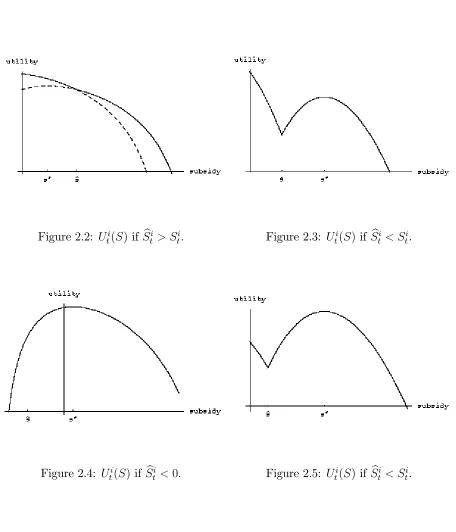
(34) 2.3 Political Equilibrium. 28. the utility at St = 0 in case of remaining uneducated, UtU (St = 0). Thus, an individual i prefers Sti to St = 0 if and only if the following inequality holds: UtE (Sti ) ≥ UtU (St = 0).. (2.17). From (2.17) it follows that an individual i prefers the subsidy level Sti to a zero subsidy if his education cost hi is small enough. ³ hit (Sti ) = wi 1 − where e. wU wE. ´. hi ≤ e hit (Sti ),. (2.18). ¢ ¡ + Sti − θt (Sti )wi ≡ e h wE , wU , Et is the critical value of the. cost of education for individuals with a parent of type i = E, U, or alternatively, it is the education cost of the individual who is indifferent between Sti and St = 0 in each income group. Thus, a lower education cost or a higher ability raises the utility from investing in education and thus, the support for Sti against St = 0. Since education subsidies are only transferred to those who invest in education, individuals’ preferences over subsidies are non single-peaked for some individuals.17 Intuitively, single-peakedness fails to exist because at low levels of education subsidies, an individual is not willing to purchase education and thus, he prefers zero subsidies since he does not receive the subsidy but he has to pay the tax used to finance it. However, as the level of education subsidies increases, he is willing to become educated and in this case, he prefers a positive subsidy. We present different examples of individuals’ preferences over education subsidies. In Figures 2.2 and 2.3, we represent the preferences of individuals whose preferred subsidy level is St = 0, while in Figures 2.4 and 2.5 we present two different cases of individuals whose preferred subsidy is Sti .18 17. Non single-peakedness appears also when both public and private education coexist. This is because. those individuals attending private schools must opt out of publicly provided education. Stiglitz (1974) was among the first to study this problem. 18 In Figure 2, the utility function of individual i is represented by the bold curve..

(35) 2.3 Political Equilibrium. 2.3.2. 29. Figure 2.2: Uti (S) if Sbti > Sti .. Figure 2.3: Uti (S) if Sbti < Sti .. Figure 2.4: Uti (S) if Sbti < 0.. Figure 2.5: Uti (S) if Sbti < Sti .. Majority Voting Equilibrium. In this section we analyze the political equilibrium level of education subsidies. The equilibrium degree of subsidization of education is decided by majority voting. As we have.

(36) 2.3 Political Equilibrium. 30. already showed in the previous section, individuals’ preferences over education subsidies are non single-peaked.19 It is well known in the voting literature that a majority voting equilibrium may exist, even if preferences fail to be single-peaked. It is the case when preferences of individuals over the public policy satisfy a single-crossing property.20 Intuitively, this property means that it is possible to order individuals by their characteristics according to their preferences for the public policy.21 In our model, the conflict of interests among individuals regarding the preferred level of subsidization of education has two dimensions. On the one hand, high-ability individuals have a lower opportunity cost of investing in education than low-ability individuals with the same income. Thus, preferred subsidies may differ across individuals belonging to the same type of family, either educated or uneducated, due to differences in education costs. It is possible to order individuals belonging to the same parent’s type by their ability to determine their preferred subsidy, since individuals with an education cost sufficiently hit (Sti ) , i = E, U prefer Sti to St = 0, whereas those with high education small, hi ≤ e hit (Sti ) prefer a zero subsidy level. costs, hi > e. On the other hand, high-income individuals prefer lower interior subsidies than low-. income individuals, StE < StU , because their gains from redistribution are lower. However, it is not possible to determine how are the preferred education subsidies of two individuals with the same education cost hi but different parental income. The most preferred subsidy of the low-income individual may be lower or higher than the most preferred subsidy of the rich individual, depending on their income and education costs. Therefore, it is not possible to order individuals by a single characteristic to determine their preferred subsidy level, which means that in our model individuals’ preferences over education subsidies are 19. This feature implies that a majority voting may not exist. See Roberts (1977) and Gans and Smart (1996)). 21 Non single-peakedness of individuals’ preferences over tax rates to finance public education appears 20. also when both public and private education coexist. This is because those individuals attending private schools must opt out of publicly provided education. Stiglitz (1974) was among the first to study this problem..

(37) 2.3 Political Equilibrium. 31. not single-crossing. We proceed as follows: first, we provide the necessary and sufficient conditions for the existence of a majority voting equilibrium and then, we show that there always exists a majority voting equilibrium subsidy in the economy. Let define the political equilibrium level of education subsidies in the economy. This subsidy is the Condorcet winner of the voting process. Definition The Condorcet winner is the subsidy level Stc , 0 ≤ Stc ≤ Stmax , that beats any other subsidy in pairwise comparison, i.e., for all S ∈ [0, Stmax ], the fraction of agents with Uti (Stc ) ≥ Uti (S) is strictly greater than half the total number of individuals in the economy. In order to find the Condorcet winner of the political process, we define as pit , the number of individuals of each parent’s type, i = E, U, whose preferred subsidy level is Sti = arg max UtE (wi ) . These individuals are those who prefer to acquire education when the education subsidy is Sti to remain uneducated at St = 0 and they have an education hit (Sti ). Accordingly, the number of individuals of each parent’s cost small enough, hi ≤ e. hit (Sti ). type whose preferred subsidy is St = 0 are those with high education costs, hi > e U This group of individuals proportion is p0t = 1 − (pE t + pt ).. 0 U These three groups of individuals of size pE t , pt and pt respectively, are the following:. eE E - pE t = Et F (ht (St )).. hUt (StU )). - pUt = (1 − Et )F (e. E eU U hE - p0t = Et (1 − F (e t (St ))) + (1 − Et )(1 − F (ht (St ))).. In the case in which one of these three groups consists of more than half the total number of individuals in the economy, i.e., pit > 12 , i = {E, U, 0}, there exists a trivial political equilibrium subsidy, which is the subsidy preferred by this group. Intuitively, St = 0 and StE are trivial majority voting equilibria respectively if either the proportion.

(38) 2.3 Political Equilibrium. 32. of educated individuals, Et , is low or sufficiently high. We may interpret Et as the level of development of the economy. Thus, when the level of development of the economy is low, the proportion of individuals who acquire education is also low and a majority of individuals support St = 0, i.e., p0t > 12 . Conversely, StE is a trivial equilibrium when the level of development is high and the proportion of individuals born of educated parents are a majority, Et > 12 . In such an economy, a majority of individuals born of educated 1 parents acquire education and support StE against St = 0 and thus, pE t > 2.. The preferred subsidy of individuals born of uneducated parents who invest in education, StU is a trivial political equilibrium, i.e., pUt > 12 , if uneducated individuals are a majority in the economy, 1 − Et >. 1 2. and the uneducated labor wage wU is sufficiently. hUt (StU )) > 12 .22 high to allow a majority of poor individuals to acquire education, F (e. We can write the requirements that the economy must satisfy in each of these cases as. implicit conditions over the level of development of the economy Et .23 Thus, St = 0 is a hUt (StU )) < trivial equilibrium if and only if F (e. 1 2. et0 , while StE is an equilibrium and Et < E. etE . Finally, StU only appears if F (e hUt (StU )) > if Et > E. 1 2. etU . and Et < E. To characterize the non-trivial political equilibrium we consider the case in which these. groups are strictly smaller than half the total population in the economy, i.e., pit <. 1 2. for. all i. Thus, the sum of any two groups consists of more than half the total number of individuals. In order to find the political equilibrium level of education subsidies Stc , we first identify which are the candidates to be the Condorcet winner. We state a lemma that provides the necessary condition that a subsidy level must satisfy to be the Condorcet winner of the voting process.24 Lemma 2.1. If Stc is a majority voting equilibrium, then it must be a local maximum for 22. This equilibrium is not relevant empirically since it would imply that a majority of children of poor. families have access to university. 23. Note that the proportion of individuals who stricly prefer Sti , i = E, U to St = 0, F (e hit (Sti )) only. depends on period t through Et . 24 A parallel result is obtained by Fernández and Rogerson (1995)..

(39) 2.3 Political Equilibrium. 33. at least one group of individuals. Proof. Assume that no group has a local maximum at Stc , this implies that. ∂Ut (Stc ) ∂St. 6= 0. for all individuals. Since Stc is the Condorcet winner, it is strictly preferred to any other alternative by more than half the total number of individuals in the economy. Then, for more than half of individuals Stc is strictly preferred to any other alternative arbitrarily closed and smaller than Stc , i.e., Uti (Stc ) > Uti (Stc − ε). Thus, the utility of more than half the population in the economy is upward sloping at Stc . Since Stc is not a local maximum, then necessarily any alternative bigger and arbitrarily closed to Stc will be preferred to i. Stc by a majority of individuals, i.e., Uti (Stc + ε) > Ut (Stc ), and then Stc cannot be the Condorcet winner. This lemma establishes that the candidates to majority voting equilibrium are the local maxima for the groups defined above, i.e., {0, StE , StU }. Now we can prove that if a candidate beats the other two, it beats any other subsidy and therefore, it is a majority voting equilibrium. Thus, the following lemma provides the sufficient condition for a candidate to be the Condorcet winner of the voting process. Lemma 2.2. If one candidate to majority voting equilibrium,. © ª 0, StE , StU , beats the. other two candidates, it is the Condorcet winner of the majority voting process. Proof. See the Appendix.. The more intuitive case is the one in which StE , which is the most preferred subsidy for individuals born of educated parents who acquire education, is strictly preferred to both St = 0 and StU by a majority of individuals in the economy. The argument used in the proof is similar to the standard arguments in the median voter theorem. In this case, those individuals whose preferred subsidy is St = 0 and those who support StE against ¡ ¤ St = 0, they are both better off at StE than at any S ∈ StE , Stmax and they are more 1 than half the total number of individuals in the economy, since p0t + pE t > 2 . On the.

(40) 2.3 Political Equilibrium. 34. other hand, those individuals who prefer StU to St = 0 and StE to St = 0 respectively, they also prefer StE to any S ∈ (0, StE ) and they are also a majority in the economy since 1 pUt + pE t > 2.. In the case of St = 0, it is easy to check that if St = 0 beats both StE and StU , then it ¡ ¢ beats any S ∈ 0, StE , since those who prefer St = 0 to StE strictly prefer a zero subsidy ¡ ¢ ¡ ¤ to any S ∈ 0, StE and the same argument holds for any S ∈ StU , Stmax because those ¤ ¡ who support St = 0 against StU also support a zero subsidy against S ∈ StU , Stmax . £ ¤ Thus, we turn to prove that St = 0 also beats any subsidy, S ∈ StE , StU . This result holds because the increase in the support for St = 0 against S, with respect to the support for St = 0 against StE or StU , is always higher than the increase in the support for S against St = 0. Finally, it is not difficult to prove that if StU beats StE and St = 0, then it trivially beats any other education subsidy. This is because individuals born of educated parents, whether they acquire education or not, always prefer St = 0 to StU . We can show that the net gains at StU are negative for individuals born of educated parents, i.e., StU − ¡ ¢ θ StU wE < 0. Thus, if StU beats St = 0 it is required that those individuals born of. uneducated parents who strictly prefer StU to St = 0 are more than half the total number of individuals in the economy, and thus, StU is a trivial majority voting equilibrium. In the following theorem we show that there always exists a local maximum that beats the other two. Therefore, we obtain the following result: Theorem 2.1. There always exists a majority voting equilibrium in the economy. Proof. See the Appendix. In the proof of this theorem we show that there does not exist any voting cycle between the candidates and therefore, the existence of a majority voting equilibrium level of education subsidies is always guaranteed. In Lemma 2.2 we have shown that the set of non-trivial majority candidates can be © ª 0 U reduced to 0, StE since both groups pE t and pt strictly prefer St = 0 to St and they.

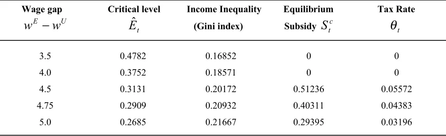
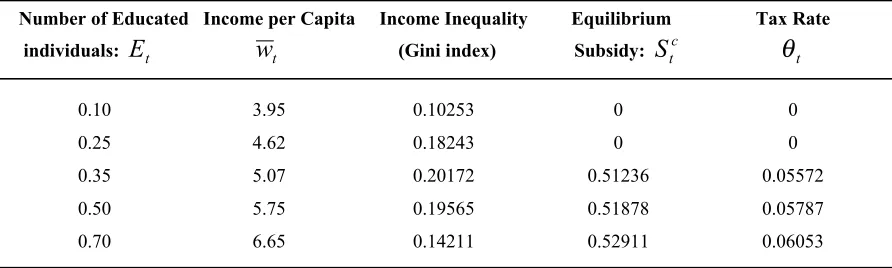
(41) 2.3 Political Equilibrium. 35. 1 0 are a majority in the economy since pE t + pt > 2 . A zero subsidy is an equilibrium when. individuals who strictly prefer St = 0 to StE are more than a half. These individuals are those born of educated and uneducated parents who obtain more utility remaining ¡ ¢ uneducated at St = 0 than acquiring education at StE , i.e., UtU (St = 0) > UtE StE and. hit (StE ), i = E, U. Conversely, StE is the equilibrium have high education costs, hi > e subsidy when the proportion of individuals of both income groups who prefer StE to. St = 0 are a majority in the economy. Thus, St = 0 is an equilibrium if the level of development of the economy is low, E eU E bt and hence, Et F (e Et < E hE t (St ))+(1 − Et ) F (ht (St )) <. 1 2. and StE is non-trivial political. bt and equilibrium if the level of development of the economy is sufficiently high, Et > E. 1 E eU E hE thus, Et F (e t (St ))+(1 − Et ) F (ht (St )) > 2 . Intuitively, these type of political equilibria. appear at intermediate levels of development compared to trivial political equilibria. Note. that the conditions that the economy must fulfilled in terms of Et are less restrictive than etE > E bt > E et0 as represented in Figure 2.6. those for trivial political equilibria since E St = 0 ~ E t0. 0 Trivial P.E.. S tE. Ê t. Et. ~ E tE. Non-trivial P.E.. 1 Trivial P.E.. Figure 2.6: Political equilibrium subsidies as a function of economic development. 2.3.3. Equilibrium Subsidies and Inequality. The size of subsidization of education not only depends on the proportion of educated individuals in the economy, Et but also on the level of income inequality. In our model,.