EM
2002 15th ASCE Engineering Mechanics ConferenceJune 2-5, 2002, Columbia University, New York, NY
APPLICATION OF THE DAMAGE INDEX METHOD TO PHASE II OF THE
ANALYTICAL SHM BENCHMARK PROBLEM
Luciana R. Barroso1, Member ASCE
and Ramses Rodriguez2
ABSTRACT
This paper presents research that utilizes the Damage Index Method to detect the location and severity of damage to the Second Phase of Analytical Studies of the Structural Health Monitoring Benchmark Problem developed by the ASCE Task Group on Structural Health Monitoring (TGoSHM). This method utilizes the ratio of curvature in the mode shape of the damaged structure vs. the undamaged structure. A shear-building model is utilized for damage detection of the unbraced frame system, both with full and partial sensor data. The location and severity of damage is carried out using the Damage Index Method for both existing damage patterns established by TGoSHM.
Keywords: damage index method, structural health monitoring, benchmark problem
INTRODUCTION
Earthquakes occurring in or near urban regions can cause severe damage to structural systems, as illustrated in recent seismic events such as those in Turkey and Taiwan. The maintenance and inspection of the affected structures can be both costly and time-consuming. Currently, engineers rely on visual inspection to detect deficiencies and estimate structural conditions. The quality of such inspections relies heavily on the knowledge and experience of the inspection crew. Another complicating factor is that damaged members may be obscured or hidden within the structure, below water, or below the ground surface.
Recent technological advances have resulted in a significant interest in development of new diagnostic techniques for monitoring the integrity of both existing and new structures in real time with minimum human involvement. To facilitate comparison between different algorithms developed to process vibration data to measure a structure’s health status, the IASC-ASCE Structural Health Monitoring Group developed a series of benchmark problems. The focus of the problem is a four-story model of an existing physical structural model at the University of British Columbia.
This research utilizes the Damage Index Method to detect the location and severity of damage to the Second Phase of Analytical Studies of the Structural Health Monitoring Benchmark Problem. This method utilizes the ratio of curvature in the mode shape of the damaged structure
1 Dept. of Civil Eng., Texas A&M University, College Station, TX 77843-3136. E-mail: [email protected]
2
vs. the undamaged structure. In addition, the Damage Index method offers the following advantages: 1) no need to unit-mass normalization of the mode shapes, 2) good results for structures in which only few modes are available (3 or less), and 3) application can be extended up to determine the structural reliability level using some statistical approach to predict consequences in terms of reliability of life of the structure. This approach has been successfully applied to identify damage to Phase I of the Analytical Studies of the Structural Health Monitoring Benchmark Problem (Barroso and Rodriguez 2002). In this study, shear-building model is utilized for damage detection of the unbraced frame system of the Phase II studies, both with full and partial sensor data.
DAMAGE DETECTION FRAMEWORK
As only the dynamic responses (i.e. accelerations) are to be utilized, the modal information must be extracted from the data. The approach selected for this problem a frequency domain decomposition approach on the undamaged response data to extract the modal parameters (Brincker et al. 2000). After the dynamic information is extracted, the Damage Index Method is utilized for damage location and severity estimates. Both methods are described in the following sections.
Extraction of Baseline from Undamaged Response Data
Modal identification from the dynamic response of the undamaged structure was performed through frequency domain decomposition (FDD) approach proposed by Brinker et al. (2000). This approach can be utilized in the presence of unknown input excitation and has been shown to be accurate even in the presence of strong noise. The power spectral density function of the
output, Gyy(jω), is calculated to be decomposed in the frequency domain through Singular Value
Decomposition (SVD) as follows:
( ) H
yy i i i i
G jw =U S U (1)
where the matrix Ui =
[
ui1, ui2, " uim]
is a unitary matrix holding the singular vectors uij, Siis a diagonal matrix holding the scalar singular values, sij, and m is the rank of the matrix Gyy(jω).
Natural frequencies are found at the corresponding peaks when plotting frequency again singular
values. Assuming a random excitation input, then the matrix Gyy(jω) can be obtained at each
frequency step as follows:
( ) ( T)( )
yy
G jω = Y Y (2)
where Y is the fast Fourier transform of the acceleration response matrix and YT is the
transpose of the complex conjugate of the matrix Y. Natural frequencies are found at the
corresponding peaks when plotting frequency again singular values.
Damage Localization and Severity: Damage Index Method
Consider a linear, undamaged structure with e elements and n nodes. The ith modal stiffness
of this structure, Ki, is given by (Stubbs et al. 1992):
T
i i i
3
where Φi is the ith modal vector and K is the system stiffness matrix. The contribution of the jth
member to the ith modal stiffness,
ij
k , is given by:
T ij i j i
k = Φ k Φ (4)
where kj is the contribution of the jth member to the system stiffness matrix. The sensitivity of
the jth member to the ith mode is determined by the fraction of the modal energy of the ith mode
that is concentrated in the jth member. This scalar value is given by:
ij ij i k F K
= (5)
The above modal parameters can be determined for both the undamaged and damaged structures, where an asterisk will indicate that the parameter refers to the damaged structure. For the damaged structure, the member sensitivity can also be expressed as follows:
1
1 e
ij
ij ij ik k
k i
k
F F A
K α ∗ ∗ ∗ = = ≅ +
∑
(6)where Aikis a set of coefficients associated with the ith element and location k, and
k
α is the
fraction of damage at location k. Dr. Stubbs et al. (1992) utilized the above information and
determined a damage indicator for the jth element,
j
β , obtained through the following:
* * * * () () 1 1 * * () () 1 1 NM e T T
i j i i k i i
i k j
j NM e
j
T T
i j i i k i i
i k
K K K
k B
k
K K K
= = = = Φ Φ + Φ Φ = = Φ Φ + Φ Φ
∑
∑
∑
∑
j=1,2...e (7)
where Kj( )contains only the geometric information of the system’s stiffness matrix (all material
properties have been filtered out). These indicators are then normalized to provide a more robust
statistical criteria for damage localization. The normalized indicator for the jth member, zj, is
given by:
(
j)
j z β β β σ −
= (8)
where β and σβ represent the mean and the standard deviation of all the indicators,
respectively.
BENCHMARK RESULTS
4
models are available: a fully braced model and a completely unbraced model. The damage patterns in the fully braced model involve the loss of stiffness in the bracing system. In contrast, the damage patterns in the unbraced model involve the loss of rotational stiffness at beam-column connections. Currently, the unbraced model has been evaluated both in the presence of both full and partial sensor information. In the partial sensor case, only the sensors
at the 2nd and 4th stories are available.
In Phase II of the benchmark problems, the complexity of the problem is incremented from Phase I in that connection flexibility is considered. The operating assumption is that joint flexibility is not known from an inspection of the drawings and is thus treated as unknown to the user. The rotational stiffness of the springs in the simulation model used to generate the problem data are equal to a nominal value multiplied by a ‘variability’, ranging from 0.75 to 1.25. While the exact amount of variability is unknown to the user, the factor is selected from a uniform distribution and is fixed by a seed value for all problem participants.
Another difference from Phase I studies lies in the mass definition. The mass on each floor differs from the nominal value by a factor, ranging from 0.9 to 1.1, which is unknown to the user. The position of the center of mass also differs somewhat from the nominal values. As the plan dimension is 2.5m by 2.5 m, the values for the eccentricities are selected from a uniform distribution with limits [-0.25m to 0.25m].
The two damage patterns defined for the structure are: (1) loss of rotational stiffness at 3 connections in level 1 and 2 connections in level 2 in each one of the perimeter frames of the strong (x-x) direction, and (2) loss of rotational stiffness at 2 connections in level 1 in each one of the perimeter frames of the strong direction. The damage identification is performed using a shear-building model, and only modal parameters from the first mode were used for the damage detection process. Each story at each face of the structure was modeled individually, resulting in a total of 4 individual shear frames as shown in Fig. 1(b).
Acceleration data records were obtained for all cases corresponding to the unbraced model with 10% RMS noise. Modal properties were extracted using the Frequency Domain Decomposition approach. The extracted natural frequencies, in Hertz, are given in Tables 1 and 2, with the results obtained from full sensor data being given in Table 1 while Table 2 gives the results obtained when only partial sensor data is available.
Table 1. Extracted Bending Natural Frequencies: Full Sensors
Undamaged Damage 1 Damage 2
Bending
Mode y-y x-x y-y x-x y-y x-x
1 3.10 4.01 3.10 3.40 3.10 3.86
2 9.75 13.23 9.75 12.78 9.75 13.23
3 16.71 25.02 16.71 24.87 16.71 25.02
4 23.51 39.54 23.51 38.78 23.51 39.09
These values correlate well with those found through the actual analytical model and given in the benchmark definition. Note that the changes in frequency in the damaged cases correspond to a decrease in stiffness in the x-x (strong) direction, where the damage occurred. Also, note that use of partial sensor data still results in very accurate estimates of the frequency. The
5
A small discrepancy is observed at higher modes, but as only 1st mode information will be
utilized in the damage identification process this error should have no impact on the results.
Table 2. Extracted Bending Natural Frequencies: Partial Sensors
Undamaged Damage 1 Damage 2
Bending
Mode y-y x-x y-y x-x y-y x-x
1 3.01 4.01 3.01 3.40 3.10 3.86 2 9.75 13.23 9.75 12.78 9.75 13.23 3 16.71 25.02 16.71 24.72 16.71 25.02
4 23.51 39.54 23.51 38.93 23.51 38.78
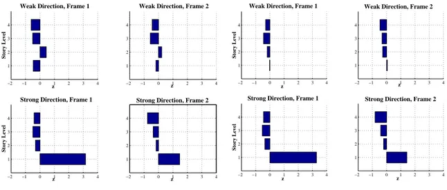
Once the modal information was extracted, the Damage Index Method was utilized to determine the location and severity of the damage. A shear-building model was utilized as the
damage identification model during this process. The normalized damage indicator, zj, was
determined and the results from these analyses are shown in Figures 1 and 2 for the full sensor cases. Damage index values greater than 1 correspond to possible damage locations. In both cases, the method accurately identifies the damage location in story level 1. In damage pattern 1, a small probability is given that damage is also found in story 2; however, that damage in incorrectly placed in the weak direction. Damage pattern 2 corresponds to a smaller degree of damage to the structure; however, the method has no difficulties identifying the damage location. The analysis based on the data from the partial sensor data gives similar results.
−2 −1 0 1 2 3 4
1 2 3 4
Story Level
−2 −1 0 1 2 3 4
1 2 3 4
−2 −1 0 1 2 3 4
1 2 3 4
Story Level
−2 −1 0 1 2 3 4
1 2 3 4
Weak Direction, Frame 1 Weak Direction, Frame 2
Strong Direction, Frame 1 Strong Direction, Frame 2
z z
z z
Fig. 1: Damage index for pattern 1
−2 −1 0 1 2 3 4
1 2 3 4
Story Level
Weak Direction, Frame 1
−2 −1 0 1 2 3 4
1 2 3 4
−2 −1 0 1 2 3 4
1 2 3 4
Story Level
−2 −1 0 1 2 3 4
1 2 3 4
Weak Direction, Frame 2
Strong Direction, Frame 1 Strong Direction, Frame 2
z z
z z
Fig. 2: Damage index for pattern 2
CONCLUSIONS
6
connected with the use of a shear-building damage identification model, which is not as sensitive to rotational information. Using a more sophisticated damage identification model that does account for rotational information should result in more accurate damage locations. Current research efforts are underway to explore the benefits of a modified damage identification model. The authors are also investigating the efficacy of this damage identification approach with a method that extracts undamaged modal information directly from the vibration data of the damaged structure.
ACKNOWLEDGMENTS
The authors would like to acknowledge the contributions from Dr. Stubbs in implementing the Damage Index Method to this problem.
REFERENCES
Barroso, L. R., and Rodriguez, R. (2002). "Stiffness-Mass Ratios Method for Baseline Determination and Damage Assessment of a Benchmark Structure." 2002 American Controls Conference, Anchorage, Alaska.
Bernal, D. (2002). "Phase II of the ASCE Benchmark Study."
http://www.ce.ust.hk/asce.shm/wp_home.asp.
Brincker, R., Zhang, L., and Andersen, P. (2000). "Modal Identification from Ambient Responses using Frequency Domain Decomposition." 18th International Modal Analysis
Conference, San Antonio, Texas, 625-630.
Stubbs, N., Kim, J.-T., and Tapole, K. (1992). "An Efficient and Robust Algorithm for Damage Localization in Offshore Platforms." ASCE 10th Structures Congress, San Antonio, Texas.
APPENDIX I. NOTATION
The following symbols are utilized in this paper:
aij = coefficients that are function of the mode shape and mass terms
A = matrix containing unknown coefficients aij
b = Vector containing eigenvalues
Gyy(jω) = power spectral density function
i
k = Lateral stiffness of ith story
K = Elastic system stiffness matrix
i
m = Mass of ith floor
M = System mass matrix
Si = Diagonal matrix holding the scalar singular values
i
U = Unitary matrix holding the singular vectors
x = Vector of the unknown stiffness to mass ratios
7 T
Y = Transpose of the complex conjugate of the matrix Y
αj = Damage severity indicator for the jth element
j
β = Damage indicator for the jth element
λ = Eigenvalue
Φ = Μode shape
j