We now study the branch of physics
con-cerned with electric and magnetic
phe-nomena. The laws of electricity and
mag-netism play a central role in the operation of
such devices as MP3 players, televisions,
elec-tric motors, computers, high-energy
accelera-tors, and other electronic devices. More
fun-damentally, the interatomic and intermolecular forces responsible for the formation of solids and
liquids are electric in origin.
Evidence in Chinese documents suggests magnetism was observed as early as 2000 BC. The
ancient Greeks observed electric and magnetic phenomena possibly as early as 700 BC. The
Greeks knew about magnetic forces from observations that the naturally occurring stone
mag-netite
(Fe
3O
4) is attracted to iron. (The word electric
comes from elecktron, the Greek word for
“amber.” The word magnetic
comes from Magnesia, the name of the district of Greece where
mag-netite was first found.)
Not until the early part of the nineteenth century did scientists establish that electricity and
magnetism are related phenomena. In 1819, Hans Oersted discovered that a compass needle is
deflected when placed near a circuit carrying an electric current. In 1831, Michael Faraday and,
almost simultaneously, Joseph Henry showed that when a wire is moved near a magnet (or,
equiv-alently, when a magnet is moved near a wire), an electric current is established in the wire. In
1873, James Clerk Maxwell used these observations and other experimental facts as a basis for
for-mulating the laws of electromagnetism as we know them today. (Electromagnetism
is a name
given to the combined study of electricity and magnetism.)
Maxwell’s contributions to the field of electromagnetism were especially significant because the
laws he formulated are basic to all
forms of electromagnetic phenomena. His work is as important
as Newton’s work on the laws of motion and the theory of gravitation.
P
ART
4
The electromagnetic force between charged particles is one of the fundamental forces of nature. We begin this chapter by describing some basic properties of one manifestation of the electromagnetic force, the electric force. We then discuss Coulomb’s law, which is the fundamental law governing the electric force between any two charged particles. Next, we introduce the concept of an electric field asso-ciated with a charge distribution and describe its effect on other charged particles. We then show how to use Coulomb’s law to calculate the electric field for a given charge distribution. The chapter concludes with a discussion of the motion of a charged particle in a uniform electric field.
23.1
Properties of Electric Charges
A number of simple experiments demonstrate the existence of electric forces. For example, after rubbing a balloon on your hair on a dry day, you will find that the balloon attracts bits of paper. The attractive force is often strong enough to sus-pend the paper from the balloon.
When materials behave in this way, they are said to be electrified or to have become electrically charged. You can easily electrify your body by vigorously rub-bing your shoes on a wool rug. Evidence of the electric charge on your body can be detected by lightly touching (and startling) a friend. Under the right condi-tions, you will see a spark when you touch and both of you will feel a slight tingle.
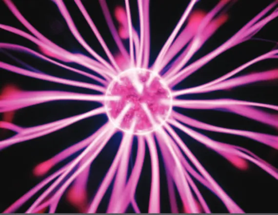
Mother and daughter are both enjoying the effects of electrically charging their bodies. Each individual hair on their heads becomes charged and exerts a repulsive force on the other hairs, resulting in the “stand-up” hair-dos seen here. (Courtesy of Resonance Research Corporation)
23.1 Properties of Electric Charges
23.2 Charging Objects by Induction
23.3 Coulomb’s Law
23.4 The Electric Field
23.5 Electric Field of a Continuous Charge Distribution
Electric Fields
23
642
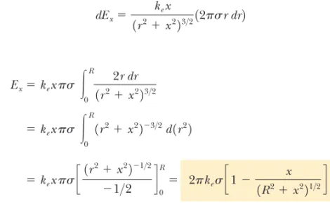
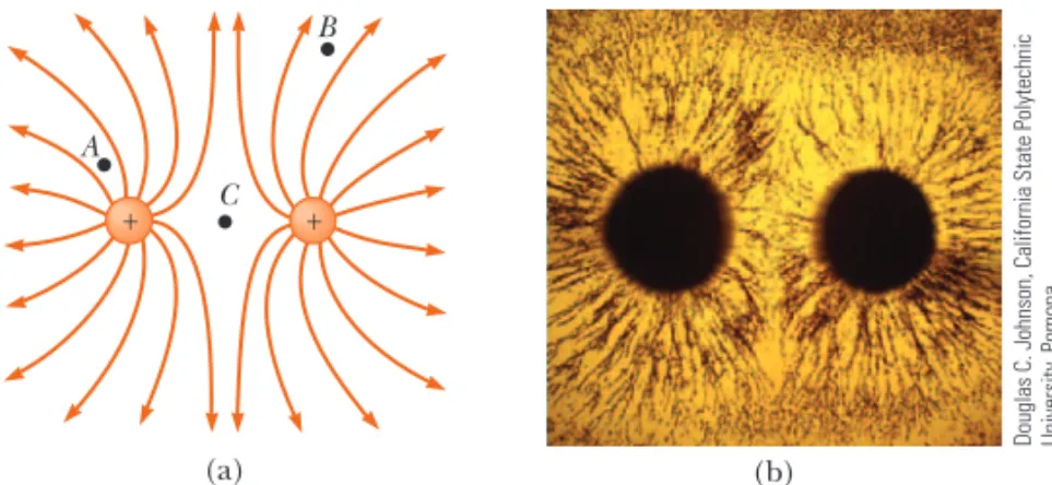
23.6 Electric Field Lines
(Experiments such as these work best on a dry day because an excessive amount of moisture in the air can cause any charge you build up to “leak” from your body to the Earth.)
In a series of simple experiments, it was found that there are two kinds of elec-tric charges, which were given the names positive and negative by Benjamin Franklin (1706–1790). Electrons are identified as having negative charge, while protons are positively charged. To verify that there are two types of charge, sup-pose a hard rubber rod that has been rubbed on fur is suspended by a sewing thread as shown in Figure 23.1. When a glass rod that has been rubbed on silk is brought near the rubber rod, the two attract each other (Fig. 23.1a). On the other hand, if two charged rubber rods (or two charged glass rods) are brought near each other as shown in Figure 23.1b, the two repel each other. This observation shows that the rubber and glass have two different types of charge on them. On the basis of these observations, we conclude that charges of the same sign repel one another and charges with opposite signs attract one another.
Using the convention suggested by Franklin, the electric charge on the glass rod is called positive and that on the rubber rod is called negative. Therefore, any charged object attracted to a charged rubber rod (or repelled by a charged glass rod) must have a positive charge, and any charged object repelled by a charged rubber rod (or attracted to a charged glass rod) must have a negative charge.
Another important aspect of electricity that arises from experimental observa-tions is that electric charge is always conservedin an isolated system. That is, when one object is rubbed against another, charge is not created in the process. The elec-trified state is due to a transferof charge from one object to the other. One object gains some amount of negative charge while the other gains an equal amount of positive charge. For example, when a glass rod is rubbed on silk as in Figure 23.2, the silk obtains a negative charge equal in magnitude to the positive charge on the glass rod. We now know from our understanding of atomic structure that electrons are transferred in the rubbing process from the glass to the silk. Similarly, when rubber is rubbed on fur, electrons are transferred from the fur to the rubber, giving the rubber a net negative charge and the fur a net positive charge. This process is consistent with the fact that neutral, uncharged matter contains as many positive charges (protons within atomic nuclei) as negative charges (electrons).
In 1909, Robert Millikan (1868–1953) discovered that electric charge always occurs as integral multiples of a fundamental amount of charge e (see Section 25.7). In modern terms, the electric charge qis said to be quantized,where qis the standard symbol used for charge as a variable. That is, electric charge exists as dis-crete “packets,” and we can write q Ne, where Nis some integer. Other experi-ments in the same period showed that the electron has a charge e and the pro-ton has a charge of equal magnitude but opposite sign e. Some particles, such as the neutron, have no charge.
Section 23.1 Properties of Electric Charges 643
Rubber
(a)
F F
(b)
F
F
Rubber
Rubber –– – – –
–– –– – –
–
+ + + +
++
Glass + – – –– –
Figure 23.1 (a) A negatively charged rubber rod suspended by a thread is attracted to a positively charged glass rod. (b) A negatively charged rubber rod is repelled by another negatively charged rubber rod.
–– – –
––
Figure 23.2 When a glass rod is rubbed with silk, electrons are trans-ferred from the glass to the silk. Because of conservation of charge, each electron adds negative charge to the silk and an equal positive charge is left behind on the rod. Also, because the charges are transferred in discrete bundles, the charges on the two objects are e, or 2e, or 3e, and so on.
Quick Quiz 23.1 Three objects are brought close to each other, two at a time. When objects A and B are brought together, they repel. When objects B and C are brought together, they also repel. Which of the following are true? (a) Objects A and C possess charges of the same sign. (b) Objects A and C possess charges of opposite sign. (c) All three objects possess charges of the same sign. (d) One object is neutral. (e) Additional experiments must be performed to determine the signs of the charges.
23.2
Charging Objects by Induction
It is convenient to classify materials in terms of the ability of electrons to move through the material:
Electrical conductors are materials in which some of the electrons are free electrons1 that are not bound to atoms and can move relatively freely
through the material; electrical insulatorsare materials in which all electrons are bound to atoms and cannot move freely through the material.
Materials such as glass, rubber, and dry wood fall into the category of electrical insulators. When such materials are charged by rubbing, only the area rubbed becomes charged and the charged particles are unable to move to other regions of the material.
In contrast, materials such as copper, aluminum, and silver are good electrical conductors. When such materials are charged in some small region, the charge readily distributes itself over the entire surface of the material.
Semiconductorsare a third class of materials, and their electrical properties are somewhere between those of insulators and those of conductors. Silicon and ger-manium are well-known examples of semiconductors commonly used in the fabri-cation of a variety of electronic chips used in computers, cellular telephones, and stereo systems. The electrical properties of semiconductors can be changed over many orders of magnitude by the addition of controlled amounts of certain atoms to the materials.
To understand how to charge a conductor by a process known as induction, consider a neutral (uncharged) conducting sphere insulated from the ground as shown in Figure 23.3a. There are an equal number of electrons and protons in the sphere if the charge on the sphere is exactly zero. When a negatively charged rub-ber rod is brought near the sphere, electrons in the region nearest the rod experi-ence a repulsive force and migrate to the opposite side of the sphere. This migra-tion leaves the side of the sphere near the rod with an effective positive charge because of the diminished number of electrons as in Figure 23.3b. (The left side of the sphere in Figure 23.3b is positively charged as ifpositive charges moved into this region, but remember that it is only electrons that are free to move.) This process occurs even if the rod never actually touches the sphere. If the same experiment is performed with a conducting wire connected from the sphere to the Earth (Fig. 23.3c), some of the electrons in the conductor are so strongly repelled by the presence of the negative charge in the rod that they move out of the sphere through the wire and into the Earth. The symbol at the end of the wire in Figure 23.3c indicates that the wire is connected to ground,which means a reservoir, such as the Earth, that can accept or provide electrons freely with negli-gible effect on its electrical characteristics. If the wire to ground is then removed 644 Chapter 23 Electric Fields
1A metal atom contains one or more outer electrons, which are weakly bound to the nucleus. When
many atoms combine to form a metal, the free electronsare these outer electrons, which are not bound to any one atom. These electrons move about the metal in a manner similar to that of gas molecules moving in a container.
(b) (a) (c) (d) (e) + + + + + + + + + + + + + + + + + + + + + + + + + + + + + + + + + + + + + + + + – – – – – – – – – – – – – –– – – – – – – – – – – – – – – – – – – – – – –
(Fig. 23.3d), the conducting sphere contains an excess of induced positive charge because it has fewer electrons than it needs to cancel out the positive charge of the protons. When the rubber rod is removed from the vicinity of the sphere (Fig. 23.3e), this induced positive charge remains on the ungrounded sphere. Notice that the rubber rod loses none of its negative charge during this process.
Charging an object by induction requires no contact with the object inducing the charge. That is in contrast to charging an object by rubbing (that is, by conduc-tion), which does require contact between the two objects.
A process similar to induction in conductors takes place in insulators. In most neutral molecules, the center of positive charge coincides with the center of nega-tive charge. In the presence of a charged object, however, these centers inside each molecule in an insulator may shift slightly, resulting in more positive charge on one side of the molecule than on the other. This realignment of charge within individual molecules produces a layer of charge on the surface of the insulator as shown in Figure 23.4a. Your knowledge of induction in insulators should help you explain why a comb that has been drawn through your hair attracts bits of electri-cally neutral paper as shown in Figure 23.4b.
Quick Quiz 23.2 Three objects are brought close to one another, two at a time. When objects A and B are brought together, they attract. When objects B and C are brought together, they repel. Which of the following are necessarily true? (a) Objects A and C possess charges of the same sign. (b) Objects A and C possess charges of opposite sign. (c) All three objects possess charges of the same sign. (d) One object is neutral. (e) Additional experiments must be performed to deter-mine information about the charges on the objects.
23.3
Coulomb’s Law
Charles Coulomb measured the magnitudes of the electric forces between charged objects using the torsion balance, which he invented (Fig. 23.5). The operating principle of the torsion balance is the same as that of the apparatus used by Cavendish to measure the gravitational constant (see Section 13.1), with the elec-trically neutral spheres replaced by charged ones. The electric force between charged spheres A and B in Figure 23.5 causes the spheres to either attract or repel each other, and the resulting motion causes the suspended fiber to twist. Because the restoring torque of the twisted fiber is proportional to the angle through which the fiber rotates, a measurement of this angle provides a quantita-tive measure of the electric force of attraction or repulsion. Once the spheres are charged by rubbing, the electric force between them is very large compared with the gravitational attraction, and so the gravitational force can be neglected.
Section 23.3 Coulomb’s Law 645
+ + +
+ + +
+ –
+ –
+ –
+ –
+ –
+ –
Wall
charges
Charged Induced
balloon (a)
Figure 23.4 (a) The charged object on the left induces a charge distribution on the surface of an insu-lator due to realignment of charges in the molecules. (b) A charged comb attracts bits of paper because charges in molecules in the paper are realigned.
© 1968 Fundamental Photographs
(b)
Suspension head
Fiber
B A
From Coulomb’s experiments, we can generalize the properties of the electric force between two stationary charged particles. We use the term point charge to refer to a charged particle of zero size. The electrical behavior of electrons and protons is very well described by modeling them as point charges. From experi-mental observations, we find that the magnitude of the electric force (sometimes called the Coulomb force) between two point charges is given by Coulomb’s law:
(23.1)
where ke is a constant called the Coulomb constant. In his experiments, Coulomb was able to show that the value of the exponent of rwas 2 to within an uncertainty of a few percent. Modern experiments have shown that the exponent is 2 to within an uncertainty of a few parts in 1016. Experiments also show that the electric force,
like the gravitational force, is conservative.
The value of the Coulomb constant depends on the choice of units. The SI unit of charge is the coulomb(C). The Coulomb constant kein SI units has the value
(23.2) This constant is also written in the form
(23.3)
where the constant P
0 (Greek letter epsilon) is known as the permittivity of free
spaceand has the value
(23.4) The smallest unit of free charge eknown in nature,2the charge on an electron
(e) or a proton (e), has a magnitude
(23.5) Therefore, 1 C of charge is approximately equal to the charge of 6.24 1018
elec-trons or protons. This number is very small when compared with the number of free electrons in 1 cm3of copper, which is on the order of 1023. Nevertheless, 1 C
is a substantial amount of charge. In typical experiments in which a rubber or glass rod is charged by friction, a net charge on the order of 106C is obtained. In
other words, only a very small fraction of the total available charge is transferred between the rod and the rubbing material.
The charges and masses of the electron, proton, and neutron are given in Table 23.1.
e1.602 181019 C P08.854 21012 C2>N#m2
ke
1 4pP0 ke8.987 610
9 N#m2>
C2 Feke
0q10 0q20 r2 646 Chapter 23 Electric Fields
CHARLES COULOMB
French physicist (1736–1806)
Coulomb’s major contributions to science were in the areas of electrostatics and magnetism. During his lifetime, he also investigated the strengths of materials and determined the forces that affect objects on beams, thereby contributing to the field of structural mechan-ics. In the field of ergonomics, his research pro-vided a fundamental understanding of the ways in which people and animals can best do work.
Photo courtesy of AIP Niels Bohr Library/E. Scott Barr Collection
Coulomb’s law
2No unit of charge smaller than ehas been detected on a free particle; current theories, however,
pro-pose the existence of particles called quarkshaving charges e/3 and 2e/3. Although there is consider-able experimental evidence for such particles inside nuclear matter, free quarks have never been detected. We discuss other properties of quarks in Chapter 46.
Coulomb constant
TABLE 23.1
Charge and Mass of the Electron, Proton, and Neutron
Particle Charge (C) Mass (kg)
Electron (e) 1.602 176 5 1019 9.109 4 1031
Proton (p) 1.602 176 5 1019 1.672 62 1027
Section 23.3 Coulomb’s Law 647
When dealing with Coulomb’s law, remember that force is a vector quantity and must be treated accordingly. Coulomb’s law expressed in vector form for the elec-tric force exerted by a charge q1on a second charge q2, written , is
(23.6) where is a unit vector directed from q1 toward q2 as shown in Active Figure 23.6a. Because the electric force obeys Newton’s third law, the electric force exerted by q2 on q1 is equal in magnitude to the force exerted by q1on q2 and in
r
^
12
F
S
12ke
q1q2 r2 r
^
12
FS12 Use Newton’s law of universal gravitation and
Table 23.1 (for the particle masses) to find the magnitude of the gravitational force:
3.61047 N
16.671011 N#m2>kg22 19.1110
31
kg2 11.671027 kg2 15.31011 m22
FgG
memp
r2 E X A M P L E 2 3 . 1
The electron and proton of a hydrogen atom are separated (on the average) by a distance of approximately 5.3 1011m. Find the magnitudes of the electric force and the gravitational force between the two particles.
SOLUTION
Conceptualize Think about the two particles separated by the very small distance given in the problem statement. In Chapter 13, we found the gravitational force between small objects to be weak, so we expect the gravitational force between the electron and proton to be significantly smaller than the electric force.
Categorize The electric and gravitational forces will be evaluated from universal force laws, so we categorize this example as a substitution problem.
The Hydrogen Atom
The ratio Fe/Fg 2 1039. Therefore, the gravitational force between charged atomic particles is negligible when compared with the electric force. Notice the similar forms of Newton’s law of universal gravitation and Coulomb’s law of electric forces. Other than magnitude, what is a fundamental difference between the two forces?
Use Coulomb’s law to find the magnitude of the electric force:
8.2108 N Feke
0e0 0e0
r2 18.9910 9
N#m2>
C22 11.6010
19 C22 15.31011 m22
r
(a)
F21
F12
q1
q2 r12
ˆ +
+
ACTIVE FIGURE 23.6
Two point charges separated by a distance rexert a force on each other that is given by Coulomb’s law. The force exerted by q2on q1is equal in magnitude and opposite in direction to the force exerted by q1on q2. (a) When the charges are of the same sign, the force is repulsive. (b) When the charges are of opposite signs, the force is attractive.
Sign in at www.thomsonedu.comand go to ThomsonNOW to move the charges to any position in two-dimensional space and observe the electric forces on them.
F
S
12
F
S
21
(b)
F21 F12
q1
q2
+
–
Vector form of Coulomb’s
the opposite direction; that is, . Finally, Equation 23.6 shows that if q1 and q2have the same sign as in Active Figure 23.6a, the product q1q2 is positive. If q1and q2 are of opposite sign as shown in Active Figure 23.6b, the product q1q2is negative. These signs describe the relativedirection of the force but not the absolute direction. A negative product indicates an attractive force, and each charge experi-ences a force toward the other. A positive product indicates a repulsive force such that each charge experiences a force away from the other. The absolutedirection of the force on a charge depends on the location of the other charge. For example, if an xaxis lies along the two charges in Active Figure 23.6a, the product q1q2 is positive, but points in the xdirection and points in the xdirection.
When more than two charges are present, the force between any pair of them is given by Equation 23.6. Therefore, the resultant force on any one of them equals the vector sum of the forces exerted by the other individual charges. For example, if four charges are present, the resultant force exerted by particles 2, 3, and 4 on particle 1 is
Quick Quiz 23.3 Object A has a charge of 2mC, and object B has a charge of 6mC. Which statement is true about the electric forces on the objects?
(a) (b) (c) (d) (e)
(f) 3F
S
ABF
S
BA
F
S
ABF
S
BA FSAB3F
S
BA 3FSAB F
S BA F S AB F S BA FSAB 3F
S
BA
F
S
1F
S
21F
S
31F
S
41 FS21 F
S
12
FS21 F
S
12 648 Chapter 23 Electric Fields
E X A M P L E 2 3 . 2
Consider three point charges located at the corners of a right triangle as shown in Figure 23.7, where q1 q3 5.0 mC, q2 2.0 mC, and a 0.10 m. Find the resultant force exerted on q3.
SOLUTION
Conceptualize Think about the net force on q3. Because charge q3 is near two other charges, it will experience two electric forces.
Categorize Because two forces are exerted on charge q3, we categorize this example as a vector addition problem.
Analyze The directions of the individual forces exerted by q1 and q2 on q3 are shown in Figure 23.7. The force exerted by q2 on q3is attractive because q2and q3have opposite signs. In the coordinate system shown in Figure 23.7, the attrac-tive force is to the left (in the negative xdirection).
The force exerted by q1on q3is repulsive because both charges are positive. The repulsive force F makes an angle of 45° with the xaxis.
S 13 F S 13 F S 23 F S 23
Find the Resultant Force
F13 q3 q1 q2 a a y x – + + F23 2a 公
Figure 23.7 (Example 23.2) The force exerted by q1on q3is . The
force exerted by q2on q3is . The resultant force exerted on q3is the vector sum F .
S
13F
S 23 F S 3 F S 23 F S 13
Use Equation 23.1 to find the magnitude of :FS23
18.99109 N#m2>
C2212.010
6 C2 15.0106 C2
10.10 m22 9.0 N F23ke
0q20 0q30 a2
Find the magnitude of the force F :
S
13
18.99109 N#m2>C22 15.010
6
C2 15.0106 C2
210.10 m22 11 N F13ke
Section 23.3 Coulomb’s Law 649
Express the resultant force acting on q3 in unit–vector form:
F
S
3 11.1i
^
7.9^j2 N
Finalize The net force on q3is upward and toward the left in Figure 23.7. If q3moves in response to the net force, the distances between q3and the other charges change, so the net force changes. Therefore, q3can be modeled as a particle under a net force as long as it is recognized that the force exerted on q3is notconstant.
What If? What if the signs of all three charges were changed to the opposite signs? How would that affect the result
for ?
Answer The charge q3 would still be attracted toward q2and repelled from q1 with forces of the same magnitude. Therefore, the final result for F would be the same.
S
3 F
S
3
Find the xand ycomponents of the force F :
S
13
F13yF13 sin 45°7.9 N F13xF13 cos 45°7.9 N
Find the components of the resultant force acting on q3:
F3yF13yF23y 7.9 N07.9 N
F3xF13xF23x7.9 N 19.0 N2 1.1 N
Analyze Write an expression for the net force on charge q3when it is in equilibrium:
FS3F
S
23F
S
13 ke
0q20 0q30 x2 i
^
ke
0q10 0q30 12.00x22 i
^
0
E X A M P L E 2 3 . 3
Three point charges lie along the x axis as shown in Figure 23.8. The positive charge q115.0 mC is at x2.00 m, the positive charge q26.00 mC is at the ori-gin, and the net force acting on q3is zero. What is the xcoordinate of q3?
SOLUTION
Conceptualize Because q3 is near two other charges, it experiences two electric forces. Unlike the preceding example, however, the forces lie along the same line in this problem as indicated in Figure 23.8. Because q3 is negative while q1 and q2 are positive, the forces and are both attractive.
Categorize Because the net force on q3 is zero, we model the point charge as a particle in equilibrium.
F
S
23 F
S
13
Where Is the Net Force Zero?
2.00 m
x
q1 x q3
q2 F23 F13
2.00 – x
+ – +
Figure 23.8 (Example 23.3) Three point charges are placed along the x axis. If the resultant force acting on q3is zero, the force exerted by q1
on q3must be equal in magnitude and opposite in direction to the force
exerted by q2on q3.
F
S
23
F
S
13
Move the second term to the right side of the equa-tion and set the coefficients of the unit vector equal:i^
ke
0q20 0q30 x2 ke
0q10 0q30 12.00x22
Eliminate ke and q3and rearrange the equation:
14.004.00xx22 16.00106 C2 x2115.0106 C2 12.00x220q20 x20q10
Reduce the quadratic equation to a simpler form: 3.00x28.00x8.000
Solve the quadratic equation for the positive root: x 0.775 m
650 Chapter 23 Electric Fields
Write Newton’s second law for the left-hand sphere in component form:
(1)
(2) aFyT cos umg0 S T cos umg
aFxT sin uFe0 S T sin uFe
What If? Suppose q3 is constrained to move only along the x axis. From its initial position at x 0.775 m, it is
pulled a small distance along the x axis. When released, does it return to equilibrium, or is it pulled further from equilibrium? That is, is the equilibrium stable or unstable?
Answer If q3 is moved to the right, becomes larger and becomes smaller. The result is a net force to the right, in the same direction as the displacement. Therefore, the charge q3would continue to move to the right and the equilibrium is unstable. (See Section 7.9 for a review of stable and unstable equilibrium.)
If q3is constrained to stay at a fixed xcoordinate but allowed to move up and down in Figure 23.8, the equilibrium is stable. In this case, if the charge is pulled upward (or downward) and released, it moves back toward the equilib-rium position and oscillates about this point.
F
S
23 F
S
13
E X A M P L E 2 3 . 4
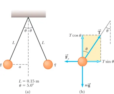
Two identical small charged spheres, each having a mass of 3.0 102 kg, hang in equilibrium as shown in Figure 23.9a.
The length of each string is 0.15 m, and the angle u is 5.0°. Find the magnitude of the charge on each sphere.
SOLUTION
Conceptualize Figure 23.9a helps us conceptualize this example. The two spheres exert repulsive forces on each other. If they are held close to each other and released, they move outward from the center and settle into the configura-tion in Figure 23.9a after the oscillaconfigura-tions have vanished due to air resistance.
Categorize The key phrase “in equilibrium” helps us model each sphere as a particle in equilibrium. This example is simi-lar to the particle in equilibrium problems in Chapter 5 with the added feature that one of the forces on a sphere is an electric force.
Analyze The free-body diagram for the left-hand sphere is shown in Figure 23.9b. The sphere is in equilibrium under the application of the forces from the string, the electric force from the other sphere, and the gravita-tional force mgS.
F
S e
T
S
Find the Charge on the Spheres
(a) (b)
mg L
L
L 0.15 m
5.0
q
a q
T T cos
T sinu
Fe u
u
u
u u
u
Figure 23.9 (Example 23.4) (a) Two identical spheres, each carrying the same charge q, suspended in equilibrium. (b) The free-body diagram for the sphere on the left of part (a).
Divide Equation (1) by Equation (2) to find Fe: tan u
Fe
mg S Femg tan u
Evaluate the electric force numerically: Fe 13.0102 kg2 19.80 m>s22tan 15.0°22.6102 N
Use the geometry of the right triangle in Figure 23.9a to find a relationship between a, L, and u:
sin u a
L S aL sin u
Evaluate a: a 10.15 m2 sin 15.0°20.013 m
Solve Coulomb’s law (Eq. 23.1) for the charge q on each sphere:
Feke
0q02
r2 S 0q0 B Fer2
ke
BFe12a22
23.4
The Electric Field
Two field forces—the gravitational force in Chapter 13 and the electric force here—have been introduced into our discussions so far. As pointed out earlier, field forces can act through space, producing an effect even when no physical con-tact occurs between interacting objects. The gravitational field at a point in space due to a source particle was defined in Section 13.4 to be equal to the gravitational force acting on a test particle of mass m divided by that mass: . The concept of a field was developed by Michael Faraday (1791–1867) in the context of electric forces and is of such practical value that we shall devote much attention to it in the next several chapters. In this approach, an electric fieldis said to exist in the region of space around a charged object, the source charge. When another charged object—the test charge—enters this electric field, an electric force acts on it. As an example, consider Figure 23.10, which shows a small positive test charge q0 placed near a second object carrying a much greater positive charge Q. We define the electric field due to the source charge at the location of the test charge to be the electric force on the test charge per unit charge, or, to be more specific, the electric field vector at a point in space is defined as the electric force act-ing on a positive test charge q0placed at that point divided by the test charge:3
(23.7)
The vector has the SI units of newtons per coulomb (N/C). Note that is the field produced by some charge or charge distribution separate fromthe test charge; it is not the field produced by the test charge itself. Also note that the existence of an electric field is a property of its source; the presence of the test charge is not necessary for the field to exist. The test charge serves as a detector of the electric field.
The direction of as shown in Figure 23.10 is the direction of the force a posi-tive test charge experiences when placed in the field. An electric field exists at a point if a test charge at that point experiences an electric force.
E
S
E
S
E
S
ES F
S e
q0
F
S e
E
S
g
S
F
S g>m
F
S g
g
S
Section 23.4 The Electric Field 651
Finalize We cannot determine the sign of the charge from the information given. In fact, the sign of the charge is not important. The situation is the same whether both spheres are positively charged or negatively charged.
What If? Suppose your roommate proposes solving this problem without the assumption that the charges are of
equal magnitude. She claims the symmetry of the problem is destroyed if the charges are not equal, so the strings would make two different angles with the vertical and the problem would be much more complicated. How would you respond?
Answer The symmetry is not destroyed and the angles are not different. Newton’s third law requires the magni-tudes of the electric forces on the two charges to be the same, regardless of the equality or nonequality of the charges. The solution to the example remains the same with one change: the value of q2in the solution is replaced
by q1q2in the new situation, where q1and q2are the values of the charges on the two spheres. The symmetry of the problem would be destroyed if the massesof the spheres were not the same. In this case, the strings would make dif-ferent angles with the vertical and the problem would be more complicated.
Substitute numerical values: 0q0 B12.610
2 N2 3210.013 m2 42
8.99109 N#m2>
C2 4.410
8 C
+ + +
+ + + + + +
+ +
+ + +
+
Q
P
Test charge Source charge
q0
E
Figure 23.10 A small positive test charge q0placed at point Pnear an
object carrying a much larger positive charge Qexperiences an electric field at point Pestablished by the source charge Q.
E
S
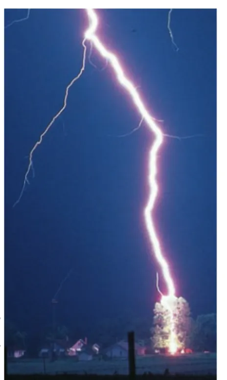
This dramatic photograph captures a lightning bolt striking a tree near some rural homes. Lightning is asso-ciated with very strong electric fields in the atmosphere.
© Johnny Autery
3When using Equation 23.7, we must assume the test charge q
0is small enough that it does not disturb
the charge distribution responsible for the electric field. If the test charge is great enough, the charge on the metallic sphere is redistributed and the electric field it sets up is different from the field it sets up in the presence of the much smaller test charge.
Equation 23.7 can be rearranged as
(23.8) This equation gives us the force on a charged particle qplaced in an electric field. If qis positive, the force is in the same direction as the field. If qis negative, the force and the field are in opposite directions. Notice the similarity between Equa-tion 23.8 and the corresponding equaEqua-tion for a particle with mass placed in a grav-itational field, (Section 5.5). Once the magnitude and direction of the electric field are known at some point, the electric force exerted on anycharged particle placed at that point can be calculated from Equation 23.8.
To determine the direction of an electric field, consider a point charge qas a source charge. This charge creates an electric field at all points in space surround-ing it. A test charge q0is placed at point P, a distance rfrom the source charge, as in Active Figure 23.11a. We imagine using the test charge to determine the direc-tion of the electric force and therefore that of the electric field. According to Coulomb’s law, the force exerted by qon the test charge is
where is a unit vector directed from q toward q0. This force in Active Figure 23.11a is directed away from the source charge q. Because the electric field at P, the position of the test charge, is defined by , the electric field at P cre-ated by qis
(23.9) If the source charge qis positive, Active Figure 23.11b shows the situation with the test charge removed: the source charge sets up an electric field at P, directed away from q. If qis negative, as in Active Figure 23.11c, the force on the test charge is toward the source charge, so the electric field at P is directed toward the source charge as in Active Figure 23.11d.
To calculate the electric field at a point P due to a group of point charges, we first calculate the electric field vectors at P individually using Equation 23.9 and then add them vectorially. In other words, at any point P, the total electric field due to a group of source charges equals the vector sum of the electric fields of all the charges. This superposition principle applied to fields follows directly from the vector addition of electric forces. Therefore, the electric field at point P due to a group of source charges can be expressed as the vector sum
(23.10) E
S
kea
i
qi
ri2
r^ i
E
S
ke
q r2 r
^
E
S
F
S e>q0 r
ˆ
F
S eke
qq0 r2 r
^
F
S
gmg
S
FSeqE S
652 Chapter 23 Electric Fields
PITFALL PREVENTION 23.1
Particles Only
Equation 23.8 is only valid for a particleof charge q, that is, an object of zero size. For a charged objectof finite size in an electric field, the field may vary in magni-tude and direction over the size of the object, so the corresponding force equation may be more complicated.
ACTIVE FIGURE 23.11 A test charge q0at point Pis a dis-tance rfrom a point charge q. (a) If qis positive, the force on the test charge is directed away from q. (b) For the positive source charge, the electric field at Ppoints radially outward from q. (c) If qis negative, the force on the test charge is directed toward q. (d) For the nega-tive source charge, the electric field at Ppoints radially inward toward q.
Sign in at www.thomsonedu.comand go to ThomsonNOW to move point P to any position in two-dimensional space and observe the electric field due to q.
(b)
E
q
P r
ˆ
(a)
Fe
q
q0
r P r
ˆ
+ +
P
(c)
Fe
q
q0
P
r
ˆ
(d)
E
q r
ˆ – –
Electric field due to a finite
Charges q1and q2are located on the xaxis, at distances a and b, respectively, from the origin as shown in Figure 23.12.
(A) Find the components of the net electric field at the point P, which is on the yaxis.
SOLUTION
Conceptualize Compare this example to Example 23.2. There, we add vector forces to find the net force on a charged particle. Here, we add electric field vectors to find the net electric field at a point in space.
Categorize We have two source charges and wish to find the resultant electric field, so we categorize this example as one in which we can use the superposition principle represented by Equation 23.10.
where riis the distance from the ith source charge qito the point Pand is a unit vector directed from qitoward P.
In Example 23.5, we explore the electric field due to two charges using the superposition principle. Part (B) of the example focuses on an electric dipole, which is defined as a positive charge qand a negative charge qseparated by a dis-tance 2a. The electric dipole is a good model of many molecules, such as hydrochloric acid (HCl). Neutral atoms and molecules behave as dipoles when placed in an external electric field. Furthermore, many molecules, such as HCl, are permanent dipoles. The effect of such dipoles on the behavior of materials subjected to electric fields is discussed in Chapter 26.
Quick Quiz 23.4 A test charge of 3 mC is at a point P where an external elec-tric field is directed to the right and has a magnitude of 4 106N/C. If the test
charge is replaced with another test charge of 3 mC, what happens to the exter-nal electric field at P? (a) It is unaffected. (b) It reverses direction. (c) It changes in a way that cannot be determined.
r
^ i
Section 23.4 The Electric Field 653
E X A M P L E 2 3 . 5 Electric Field Due to Two Charges
Analyze Find the magnitude of the electric field at Pdue to charge q1:
E1ke
0q10 r1˛
2 ke
0q10 1a2y22
Find the magnitude of the electric field at P due to charge q2:
E2ke
0q20 r2˛
2 ke
0q20 1b2y22
Write the electric field vectors for each charge in unit–vector form:
ES2ke
0q20
1b2y22 cos u i
^
ke
0q20
1b2y22 sin u j
^
E
S
1ke
0q10
1a2y22 cos f i
^
ke
0q10
1a2y22 sin f j
^
Write the components of the net electric field vector:
(1)
(2) EyE1yE2y ke
0q10
1a2y22 sin fke 0q20
1b2y22 sin u ExE1xE2x ke
0q10
1a2y22 cos fke 0q20
1b2y22 cos u f
f u
u P
y
x b
a –
+
E
E2 E1
q r2 r1
2 q1
Figure 23.12 (Example 23.5) The total electric field at Pequals the vector sum , where is the field due to the positive charge q1 and is the field due to the nega-tive charge q2.
E
S
2
E
S
1
E
S
1E
S
2
23.5
Electric Field of a Continuous
Charge Distribution
Very often, the distances between charges in a group of charges are much smaller than the distance from the group to a point where the electric field is to be calcu-lated. In such situations, the system of charges can be modeled as continuous. That is, the system of closely spaced charges is equivalent to a total charge that is 654 Chapter 23 Electric Fields
SOLUTION
In the solution to part (B), because y W a, neglect a2 compared with y2 and write the expression for Ein this
case:
(5) E ke
2qa y3
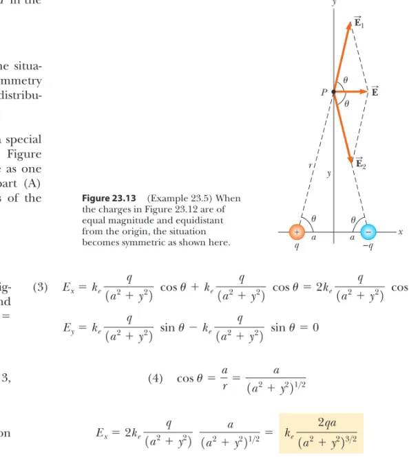
Finalize From Equation (5), we see that at points far from a dipole but along the perpendicular bisector of the line joining the two charges, the magnitude of the electric field created by the dipole varies as 1/r3, whereas the more
slowly varying field of a point charge varies as 1/r2(see Eq. 23.9). That is because at distant points, the fields of the
two charges of equal magnitude and opposite sign almost cancel each other. The 1/r3 variation in Efor the dipole
also is obtained for a distant point along the xaxis (see Problem 18) and for any general distant point.
P E
y E1
E2 y r
a
q a –q
x
+ –
u
u
u u
Figure 23.13 (Example 23.5) When the charges in Figure 23.12 are of equal magnitude and equidistant from the origin, the situation becomes symmetric as shown here.
(B)Evaluate the electric field at point Pin the special case that q1= q2and a= b.
SOLUTION
Conceptualize Figure 23.13 shows the situa-tion in this special case. Notice the symmetry in the situation and that the charge distribu-tion is now an electric dipole.
Categorize Because Figure 23.13 is a special case of the general case shown in Figure 23.12, we can categorize this example as one in which we can take the result of part (A) and substitute the appropriate values of the variables.
Analyze Based on the symmetry in Fig-ure 23.13, evaluate Equations (1) and (2) from part (A) with ab, q1q2 q, and fu:
(3)
Eyke
q
1a2y22 sin uke q
1a2y22 sin u0 Exke
q
1a2y22 cos uke
q
1a2y22 cos u2ke
q
1a2y22 cos u
From the geometry in Figure 23.13, evaluate cos u:
(4) cos u a r
a 1a2y221>2
Substitute Equation (4) into Equation (3):
Ex2ke
q 1a2y22
a
1a2y221>2 ke
2qa 1a2y223>2
continuously distributed along some line, over some surface, or throughout some volume.
To set up the process for evaluating the electric field created by a continuous charge distribution, let’s use the following procedure. First, divide the charge dis-tribution into small elements, each of which contains a small charge qas shown in Figure 23.14. Next, use Equation 23.9 to calculate the electric field due to one of these elements at a point P. Finally, evaluate the total electric field at P due to the charge distribution by summing the contributions of all the charge elements (that is, by applying the superposition principle).
The electric field at Pdue to one charge element carrying charge qis
where r is the distance from the charge element to point P and is a unit vector directed from the element toward P. The total electric field at P due to all ele-ments in the charge distribution is approximately
where the index irefers to the ith element in the distribution. Because the charge distribution is modeled as continuous, the total field at Pin the limit qiS0 is
(23.11)
where the integration is over the entire charge distribution. The integration in Equation 23.11 is a vector operation and must be treated appropriately.
Let’s illustrate this type of calculation with several examples in which the charge is distributed on a line, on a surface, or throughout a volume. When performing such calculations, it is convenient to use the concept of a charge densityalong with the following notations:
■ If a charge Q is uniformly distributed throughout a volume V, the volume charge densityris defined by
where rhas units of coulombs per cubic meter (C/m3).
■ If a charge Q is uniformly distributed on a surface of area A, the surface charge densitys(Greek letter sigma) is defined by
where shas units of coulombs per square meter (C/m2).
■ If a charge Q is uniformly distributed along a line of length , the linear charge densitylis defined by
where lhas units of coulombs per meter (C/m).
■ If the charge is nonuniformly distributed over a volume, surface, or line, the amounts of charge dqin a small volume, surface, or length element are
dqrdV dqsdA dqld/
l Q
/
s Q A r Q V ESke lim
¢qiS0ai
¢qi ri2
r^ ike
dq r2 r
^
E
S
kea
i
¢qi ri2
r^ i
r
^
¢E
S
ke
¢q r2 r
^
Section 23.5 Electric Field of a Continuous Charge Distribution 655
r
q rˆ
P
E
Figure 23.14 The electric field at P due to a continuous charge distribu-tion is the vector sum of the fields due to all the elements qof the charge distribution.
E
S
Electric field due to a
con-tinuous charge distribution
Volume charge density
Surface charge density
656 Chapter 23 Electric Fields
P R O B L E M - S O LV I N G S T R AT E G Y
The following procedure is recommended for solving problems that involve the determination of an electric field due to individual charges or a charge distribution:
1. Conceptualize. Establish a mental representation of the problem: think carefully about the individual charges or the charge distribution and imagine what type of electric field they would create. Appeal to any symmetry in the arrangement of charges to help you visualize the electric field.
2. Categorize. Are you analyzing a group of individual charges or a continuous charge distribution? The answer to this question tells you how to proceed in the Analyze step.
3. Analyze.
(a)If you are analyzing a group of individual charge, use the superposition princi-ple: When several point charges are present, the resultant field at a point in space is the vector sumof the individual fields due to the individual charges (Eq. 23.10). Be very careful in the manipulation of vector quantities. It may be useful to review the material on vector addition in Chapter 3. Example 23.5 demonstrated this procedure.
(b)If you are analyzing a continuous charge distribution,replace the vector sums for evaluating the total electric field from individual charges by vector integrals. The charge distribution is divided into infinitesimal pieces, and the vector sum is carried out by integrating over the entire charge distribution (Eq. 23.11). Examples 23.6 through 23.8 demonstrate such procedures.
Consider symmetry when dealing with either a distribution of point charges or a continuous charge distribution. Take advantage of any symmetry in the sys-tem you observed in the Conceptualize step to simplify your calculations. The cancellation of field components perpendicular to the axis in Example 23.7 is an example of the application of symmetry.
4. Finalize.Check to see if your electric field expression is consistent with the men-tal representation and if it reflects any symmetry that you noted previously. Imagine varying parameters such as the distance of the observation point from the charges or the radius of any circular objects to see if the mathematical result changes in a reasonable way.
Calculating the Electric Field
E X A M P L E 2 3 . 6
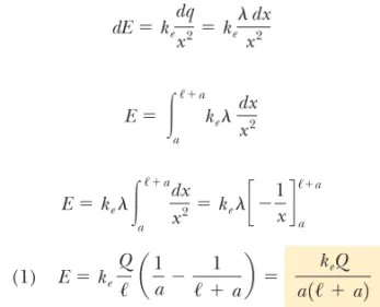
A rod of length has a uniform positive charge per unit length l
and a total charge Q. Calculate the electric field at a point Pthat is located along the long axis of the rod and a distance afrom one end (Fig. 23.15).
SOLUTION
Conceptualize The field at Pdue to each segment of charge on the rod is in the negative x direction because every segment carries a positive charge.
Categorize Because the rod is continuous, we are evaluating the field due to a continuous charge distribution rather than a group
of individual charges. Because every segment of the rod produces an electric field in the negative xdirection, the sum of their contributions can be handled without the need to add vectors.
Analyze Let’s assume the rod is lying along the xaxis, dxis the length of one small segment, and dqis the charge on that segment. Because the rod has a charge per unit length l, the charge dqon the small segment is dqldx.
dES
The Electric Field Due to a Charged Rod
x y
a
P
x dx
dq = dx
E
l
Figure 23.15 (Example 23.6) The electric field at Pdue to a uniformly charged rod lying along the xaxis. The magnitude of the field at Pdue to the segment of charge dqis kedq/x2. The total field at Pis the vector sum over all
Section 23.5 Electric Field of a Continuous Charge Distribution 657
Find the magnitude of the electric field at Pdue to one segment of the rod having a charge dq:
dEke
dq x2ke
ldx x2
Finalize If goes to zero, Equation (1) reduces to the electric field due to a point charge as given by Equation 23.9, which is what we expect because the rod has shrunk to zero size.
What If? Suppose point Pis very far away from the rod. What is the nature of the electric field at such a point?
Answer If P is far from the rod (a W ), then in the denominator of Equation (1) can be neglected and E keQ/a2. That is exactly the form you would expect for a point charge. Therefore, at large values of a/, the charge distribution appears to be a point charge of magnitude Q; the point P is so far away from the rod we cannot distinguish that it has a size. The use of the limiting technique (a/ S ) is often a good method for checking a mathematical expression.
Find the total field at Pusing4Equation 23.11: E
/a
a
kel
dx x2
Noting that ke and l Q/ are constants and can be removed from the integral, evaluate the integral:
(1) Eke
Q / a
1 a
1
/ab keQ
a1/a2 Ekel
/a
a
dx
x2 kelc
1 xd
/a
a
4To carry out integrations such as this one, first express the charge element dqin terms of the other variables in the integral. (In this example,
there is one variable, x, so we made the change dqldx.) The integral must be over scalar quantities; therefore, express the electric field in terms of components, if necessary. (In this example, the field has only an xcomponent, so this detail is of no concern.) Then, reduce your expres-sion to an integral over a single variable (or to multiple integrals, each over a single variable). In examples that have spherical or cylindrical sym-metry, the single variable is a radial coordinate.
E X A M P L E 2 3 . 7
A ring of radius acarries a uniformly distributed positive total charge Q. Calculate the electric field due to the ring at a point Plying a distance xfrom its center along the central axis perpendi-cular to the plane of the ring (Fig. 23.16a).
SOLUTION
Conceptualize Figure 23.16a shows the electric field contribution at P due to a single seg-ment of charge at the top of the ring. This field vector can be resolved into components dEx par-allel to the axis of the ring and dE›
perpendicu-lar to the axis. Figure 23.16b shows the electric field contributions from two segments on
oppo-site sides of the ring. Because of the symmetry of the situation, the perpendicular components of the field cancel. That is true for all pairs of segments around the ring, so we can ignore the perpendicular component of the field and focus solely on the parallel components, which simply add.
Categorize Because the ring is continuous, we are evaluating the field due to a continuous charge distribution rather than a group of individual charges.
dE
S
The Electric Field of a Uniform Ring of Charge
u
(a)
+ + +
+ + +
+ + +
+ + +
+ +
+ +
P dE x
dE dE› x
r dq
a
Figure 23.16 (Example 23.7) A uniformly charged ring of radius a. (a) The field at Pon the xaxis due to an element of charge dq. (b) The total electric field at Pis along the xaxis. The perpendicular component of the field at Pdue to segment 1 is canceled by the perpendicular component due to segment 2.
u x
(b)
+ + +
+ +
+ + + +
+ + +
+ + + +
dE2
1
dE1
658 Chapter 23 Electric Fields
E X A M P L E 2 3 . 8
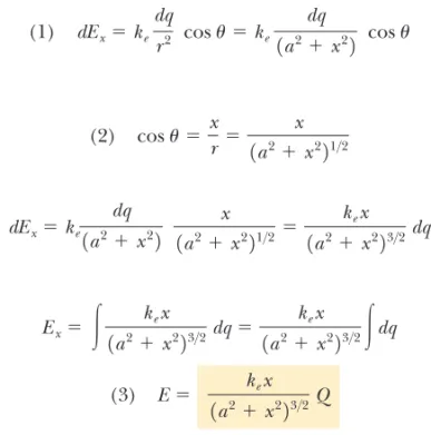
A disk of radius Rhas a uniform surface charge density s. Calculate the electric field at a point P that lies along the central perpendicular axis of the disk and a distance xfrom the center of the disk (Fig. 23.17).
SOLUTION
Conceptualize If the disk is considered to be a set of concentric rings, we can use our result from Example 23.7—which gives the field created by a ring of radius a—and sum the contributions of all rings making up the disk. By symmetry, the field at an axial point must be along the central axis.
Categorize Because the disk is continuous, we are evaluating the field due to a continuous charge distribution rather than a group of individual charges.
The Electric Field of a Uniformly Charged Disk
Analyze Evaluate the parallel component of an elec-tric field contribution from a segment of charge dq on the ring:
(1) dExke
dq
r2 cos uke
dq
1a2x22 cos u
From the geometry in Figure 23.16a, evaluate cos u: (2) cos u x r
x 1a2x221>2
Substitute Equation (2) into Equation (1): dExke
dq 1a2x22
x
1a2x221>2
kex
1a2x223>2dq
All segments of the ring make the same contribution to the field at P because they are all equidistant from this point. Integrate to obtain the total field at P:
(3) E kex 1a2x223>2Q Ex
kex
1a2x223>2dq
kex
1a2x223>2
dqFinalize This result shows that the field is zero at x 0. Is that consistent with the symmetry in the problem? Fur-thermore, notice that Equation (3) reduces to keQ/x2if xWa, so the ring acts like a point charge for locations far away from the ring.
What If? Suppose a negative charge is placed at the center of the ring in Figure 23.16 and displaced slightly by a
distance xVaalong the xaxis. When the charge is released, what type of motion does it exhibit?
Answer In the expression for the field due to a ring of charge, let xVa, which results in
Therefore, from Equation 23.8, the force on a charge qplaced near the center of the ring is
Because this force has the form of Hooke’s law (Eq. 15.1), the motion of the negative charge is simple harmonic! Fx
keqQ
a3 x Ex
keQ
a3 x
P x r
R dq
dr
Figure 23.17 (Example 23.8) A uni-formly charged disk of radius R. The electric field at an axial point Pis directed along the central axis, per-pendicular to the plane of the disk.
Analyze Find the amount of charge dq on a ring of radius rand width dras shown in Figure 23.17:
23.6
Electric Field Lines
We have defined the electric field mathematically through Equation 23.7. Let’s now explore a means of visualizing the electric field in a pictorial representation. A convenient way of visualizing electric field patterns is to draw lines, called elec-tric field linesand first introduced by Faraday, that are related to the electric field in a region of space in the following manner:
■ The electric field vector is tangent to the electric field line at each point. The line has a direction, indicated by an arrowhead, that is the same as that of the electric field vector. The direction of the line is that of the force on a positive test charge placed in the field.
■ The number of lines per unit area through a surface perpendicular to the lines is proportional to the magnitude of the electric field in that region. Therefore, the field lines are close together where the electric field is strong and far apart where the field is weak.
These properties are illustrated in Figure 23.18. The density of field lines through surface A is greater than the density of lines through surface B. There-fore, the magnitude of the electric field is larger on surface A than on surface B. Furthermore, because the lines at different locations point in different directions, the field is nonuniform.
Is this relationship between strength of the electric field and the density of field lines consistent with Equation 23.9, the expression we obtained for E using Coulomb’s law? To answer this question, consider an imaginary spherical surface of radius rconcentric with a point charge. From symmetry, we see that the magni-tude of the electric field is the same everywhere on the surface of the sphere. The number of lines Nthat emerge from the charge is equal to the number that pene-trate the spherical surface. Hence, the number of lines per unit area on the sphere is N/4pr2(where the surface area of the sphere is 4pr2). Because Eis
pro-portional to the number of lines per unit area, we see that E varies as 1/r2; this
finding is consistent with Equation 23.9. E
S
Section 23.6 Electric Field Lines 659
To obtain the total field at P, integrate this expres-sion over the limits r 0 to r R, noting that xis a constant in this situation:
kexpsc
1r2x221>2 1>2 d
R
0
2pkesc1
x 1R2x221>2d
kexps
R
0
1r2x223>2d1r22 Exkexps
R
0
2rdr 1r2x223>2
Finalize This result is valid for all values of x 0. We can calculate the field close to the disk along the axis by assuming that RWx; therefore, the expression in brackets reduces to unity to give us the near-field approximation
where P
0is the permittivity of free space. In Chapter 24, we obtain the same result for the field created by an infinite
plane of charge with uniform surface charge density.
Ex2pkes
s
2P0 Use this result in the equation given for Exin
Exam-ple 23.7 (with areplaced by rand Qreplaced by dq) to find the field due to the ring:
dEx
kex
1r2x223>212psrdr2
B A