Composition and energy determination in cosmic ray surface arrays: an application to the Pierre Auger Observatory

Texto completo

(1)Universidad de Alcalá DEPARTAMENTO DE FÍSICA. TESIS DOCTORAL. Composition and energy determination in cosmic ray surface arrays: an application to the Pierre Auger Observatory Dirigida por los doctores: L. del Peral Gochicoa, G. A. Medina Tanco, M. D. Rodrı́guez Frı́as y F. Arqueros Martı́nez.. Germán Ros Magán Alcalá de Henares. Septiembre de 2009..

(2)

(3) Universidad de Alcalá DEPARTAMENTO DE FÍSICA. Composition and energy determination in cosmic ray surface arrays: an application to the Pierre Auger Observatory. Memoria presentada para optar al Grado de Doctor en Fı́sica por: Germán Ros Magán Alcalá de Henares. Septiembre de 2009.. Fdo: Germán Ros Magán.

(4)

(5) Agradecimientos El camino recorrido durante estos años, hasta llegar aquı́, ha sido muy gratificante, tanto por el desafı́o personal que ha supuesto en todo momento como por la gente que he tenido la oportunidad de conocer. Al comienzo de esta aventura, uno no sabe dónde se mete ni hacia dónde le conducirá, pero para mı́, a pesar de las dificultades y de algunos momentos duros, ha sido la mejor experiencia de mi vida y ha estado repleta de regalos. Primero y ante todo, he de dar las gracias a mi familia: a mis padres que me han permitido seguir el camino que he querido, dándome todo su apoyo y que se han preocupado tanto o más que yo en algunos momentos; y, por supuesto, a mi hermano y a mis abuelos, a los que tanto necesito. A Luis y a Loly, mis directores de tesis en el dı́a a dı́a en la Universidad de Alcalá, agradecerles la confianza que han depositado en mı́, por guiarme, ayudarme en todo lo que está en su mano y por haber conseguido siempre lo mejor para mı́. Me gustarı́a agradecer también a Fernando, por quien me inicié en el mundo de la investigación y llegué a esto de los rayos cósmicos. A Gustavo, he de agradecerle muchas cosas, entre ellas el haber sabido sacar lo mejor de mı́ y haber creı́do en mı́ más que yo mismo, indicándome el camino correcto, ofreciéndome su apoyo. Además, me ha dado su amistad y me ha abierto la puerta al grupo de gente que he conocido en la UNAM y en México, que tanto significan para mı́. Aprovecho para dar las gracias a todos ellos: Marat, Mané, Chamı́n, Daniel, Andrea, Fede, Gabi, Cinzia, Natalia, Alondra, Camila ... Podı́a haber sido muy difı́cil pasar 14 meses allı́, y sin embargo, han sido unos meses maravillosos gracias a todos vosotros. Quiero destacar un poquito a Marat por acogerme desde el primer dı́a, a Chamı́n por enseñarme que México i.

(6) es mucho más que el DF, a Daniel porque conocerle y trabajar al lado de una persona como él ha sido un verdadero un placer y a Natalia por haberme dedicado gran parte de su tiempo y ayudado a conocer un paı́s y una gente tan maravillosos como México. A mis amigos de siempre, a los de la Complu, muchos de los cuales están en este mismo camino, y a los nuevos que he descubierto en Ciencias durante la tesis, gracias por haber estado ahı́. Sé que puedo contar con todos vosotros. Gracias también Eduardo por haberme ayudado en la correción de la tesis y a Izas, por hacer que el inglés suene algo mejor. He de mencionar a las instituciones que me han apoyado y financiado en estos años. A la Comunidad de Madrid por la concesión de una F.P.I. y varias ayudas de viaje, al Departamento de Fı́sica y a la Universidad de Alcalá, donde he pasado la mayor parte de este tiempo siempre muy a gusto y que también ha permitido que pueda asistir a varios congresos y estancias, al programa HELEN que me ha permitido realizar diversas estancias en el extranjero que han sido muy necesarias para este resultado final y, por último, al Instituto de Ciencias Nucleares de la Universidad Nacional Autónoma de México, al que pertenezco como estudiante asociado de postgrado, que me ha acogido durante más de un año de gran provecho profesional y personal. Pero esta tesis además me tenı́a guardada una gran sorpresa, el mayor regalo, un dı́a Marı́a Ángeles entró en mi despacho y sé que no se irá nunca. Eres lo más bonito del mundo.. ii.

(7) Contents 1 Introduction. 1. 2 Ultra-high Energy Cosmic Rays. 5. 2.1. History and cosmic ray discoveries . . . . . . . . . . . . . . . . . . . . . . .. 5. 2.2. Ultra-high energy cosmic rays physics . . . . . . . . . . . . . . . . . . . . .. 7. 2.2.1. Candidate sources and acceleration mechanisms . . . . . . . . . . .. 7. 2.2.2. Is cosmic ray astronomy possible?. Propagation, magnetic fields and the GZK effect . . . . . . . . . . . . . . . . . . . . . . . . . . . 14. 2.2.3 2.3. Energy and composition . . . . . . . . . . . . . . . . . . . . . . . . 20. Extensive air showers . . . . . . . . . . . . . . . . . . . . . . . . . . . . . . 29 2.3.1. Phenomenology . . . . . . . . . . . . . . . . . . . . . . . . . . . . . 29. 2.3.2. Longitudinal development . . . . . . . . . . . . . . . . . . . . . . . 33. 2.3.3. Lateral development . . . . . . . . . . . . . . . . . . . . . . . . . . 35. 2.3.4. Detection Techniques . . . . . . . . . . . . . . . . . . . . . . . . . . 38. 3 Pierre Auger Observatory. 43. 3.1. Background and advantages of a hybrid detector . . . . . . . . . . . . . . . 43. 3.2. Surface detectors . . . . . . . . . . . . . . . . . . . . . . . . . . . . . . . . 46. 3.3. Fluorescence detectors . . . . . . . . . . . . . . . . . . . . . . . . . . . . . 48. 3.4. Composition Observables . . . . . . . . . . . . . . . . . . . . . . . . . . . . 51 3.4.1. Parameters from the fluorescence technique. 3.4.2. Parameters from the surface detectors iii. . . . . . . . . . . . . . 51. . . . . . . . . . . . . . . . . 53.

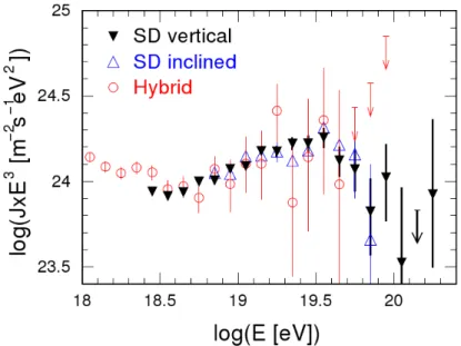
(8) CONTENTS 3.4.3 3.5. Why the issue of composition is so difficult? . . . . . . . . . . . . . 61. Pierre Auger South Observatory: Results . . . . . . . . . . . . . . . . . . . 64 3.5.1. UHECRs: spectrum. . . . . . . . . . . . . . . . . . . . . . . . . . . 64. 3.5.2. UHECRs: composition . . . . . . . . . . . . . . . . . . . . . . . . . 66. 3.5.3. Upper limit on the diffuse flux of ultra-high energy neutrinos . . . . 72. 3.5.4. Search for UHECR sources and anisotropies . . . . . . . . . . . . . 74. 4 Optimum distance in surface arrays. 79. 4.1. Motivation . . . . . . . . . . . . . . . . . . . . . . . . . . . . . . . . . . . . 80. 4.2. Algorithm to determine the optimum distance . . . . . . . . . . . . . . . . 83. 4.3. ropt dependencies on energy, zenith angle and array size . . . . . . . . . . . 88. 4.4. Influence of ropt on the reconstructed energy . . . . . . . . . . . . . . . . . 94. 4.5. 4.4.1. Energy error distribution functions . . . . . . . . . . . . . . . . . . 95. 4.4.2. Bias in the reconstructed energies . . . . . . . . . . . . . . . . . . . 95. 4.4.3. Reconstruction of a rapidly changing spectrum . . . . . . . . . . . . 100. Summary and discussion . . . . . . . . . . . . . . . . . . . . . . . . . . . . 105. 5 A new parameter for composition discrimination. 107. 5.1. Motivation . . . . . . . . . . . . . . . . . . . . . . . . . . . . . . . . . . . . 108. 5.2. Analytical study. 5.3. . . . . . . . . . . . . . . . . . . . . . . . . . . . . . . . . 110. 5.2.1. Optimization assuming Auger tanks . . . . . . . . . . . . . . . . . . 112. 5.2.2. Modifying the slope of the LDF . . . . . . . . . . . . . . . . . . . . 114. 5.2.3. Modifying the muon content of the simulated showers . . . . . . . . 116. Numerical analysis . . . . . . . . . . . . . . . . . . . . . . . . . . . . . . . 118 5.3.1. Optimization and comparison with the analytical result . . . . . . . 119. 5.3.2. Influence of the detectors far from the shower axis . . . . . . . . . . 120. 5.3.3. Energy and zenith angle dependence . . . . . . . . . . . . . . . . . 122. 5.4. Application . . . . . . . . . . . . . . . . . . . . . . . . . . . . . . . . . . . 124. 5.5. Summary . . . . . . . . . . . . . . . . . . . . . . . . . . . . . . . . . . . . 130 iv.

(9) CONTENTS 6 On-going work and perspectives. 133. 7 Conclusions and Outlook. 139. A Optimum distance at Auger North array. 147. A.1 Introduction . . . . . . . . . . . . . . . . . . . . . . . . . . . . . . . . . . . 147 A.2 Algorithm: ropt and energy determination . . . . . . . . . . . . . . . . . . . 148 A.3 ropt dependence on energy and zenith angle . . . . . . . . . . . . . . . . . . 153 A.4 Energy error distributions . . . . . . . . . . . . . . . . . . . . . . . . . . . 154 A.4.1 Shape of the energy error distributions . . . . . . . . . . . . . . . . 157 A.4.2 Bias in the reconstructed energies . . . . . . . . . . . . . . . . . . . 157 A.5 Summary and discussion . . . . . . . . . . . . . . . . . . . . . . . . . . . . 162 B Reconstruction of surface events at Auger. 165. B.1 Station and event selection . . . . . . . . . . . . . . . . . . . . . . . . . . . 166 B.2 Plane fit to the shower front . . . . . . . . . . . . . . . . . . . . . . . . . . 169 B.3 The lateral distribution function . . . . . . . . . . . . . . . . . . . . . . . . 171 B.4 Maximum Likelihood . . . . . . . . . . . . . . . . . . . . . . . . . . . . . . 172 B.5 Curvature shower front . . . . . . . . . . . . . . . . . . . . . . . . . . . . . 175 B.6 Fit stages . . . . . . . . . . . . . . . . . . . . . . . . . . . . . . . . . . . . 176 B.7 Energy estimation . . . . . . . . . . . . . . . . . . . . . . . . . . . . . . . . 177 C Resumen. 179. C.1 Antecedentes . . . . . . . . . . . . . . . . . . . . . . . . . . . . . . . . . . 179 C.2 Distancia óptima en los experimentos de superficie . . . . . . . . . . . . . . 182 C.3 Un nuevo parámetro para estudios de composición . . . . . . . . . . . . . . 186 C.4 Conclusiones . . . . . . . . . . . . . . . . . . . . . . . . . . . . . . . . . . . 192 Bibliography. 201. v.

(10)

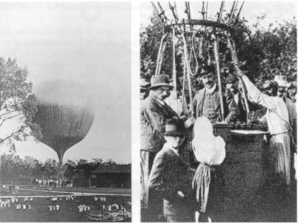
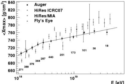
(11) List of Figures 2.1. V. Hess in the balloon flights which led to the discovery of cosmic rays . .. 7. 2.2. First and second order Fermi acceleration mechanisms . . . . . . . . . . . . 11. 2.3. Hillas Plot: possible sources of UHECRs . . . . . . . . . . . . . . . . . . . 12. 2.4. Deflection of UHECRs by magnetic fields . . . . . . . . . . . . . . . . . . . 15. 2.5. Reduction of the primary proton energy due to GZK effect . . . . . . . . . 17. 2.6. Several interactions of proton and iron nucleus with the CMB . . . . . . . 19. 2.7. Energy spectrum of cosmic rays . . . . . . . . . . . . . . . . . . . . . . . . 21. 2.8. Energy spectrum of cosmic rays measured by most of the experiments in the whole energy range . . . . . . . . . . . . . . . . . . . . . . . . . . . . . 22. 2.9. Energy spectrum of cosmic rays at the highest energies multiplied by E 2.7 . 22. 2.10 The ankle and the dip models for the transition region of the spectrum . . 25 2.11 The mixed composition model for the transition region of the spectrum . . 26 2.12 The trans-GZK recovery of the spectrum . . . . . . . . . . . . . . . . . . . 28 2.13 Sketch of an Extensive Air Shower and energy flow between different shower components . . . . . . . . . . . . . . . . . . . . . . . . . . . . . . . . . . . 31 2.14 Longitudinal development of an EAS . . . . . . . . . . . . . . . . . . . . . 35 2.15 Lateral development of an EAS . . . . . . . . . . . . . . . . . . . . . . . . 37 3.1. Picture of hybrid detection of an EAS . . . . . . . . . . . . . . . . . . . . . 45. 3.2. Layout of the Auger South Observatory . . . . . . . . . . . . . . . . . . . . 46. 3.3. An Auger surface water Cherenkov detector . . . . . . . . . . . . . . . . . 47. 3.4. Sketch of the Fluorescence Telescope . . . . . . . . . . . . . . . . . . . . . 49 vii.

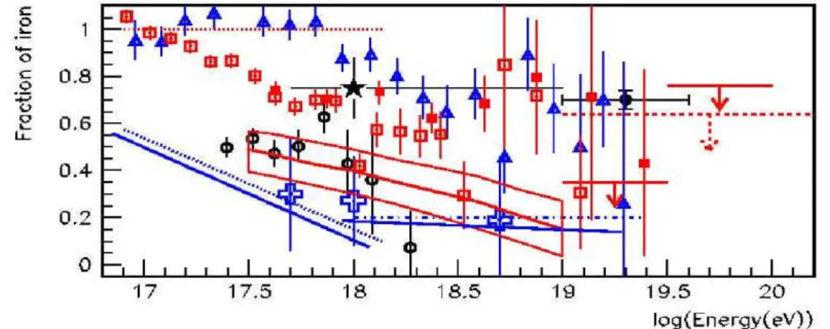
(12) LIST OF FIGURES 3.5. Camera, mirror and diaphragm of the fluorescence telescopes . . . . . . . . 50. 3.6. Elongation Rate from different experiments . . . . . . . . . . . . . . . . . . 52. 3.7. Geometrical correlation between the longitudinal development of a shower and the time structure . . . . . . . . . . . . . . . . . . . . . . . . . . . . . 55. 3.8. Rise time benchmark to determine the parameter < ∆ > . . . . . . . . . . 56. 3.9. Radius of curvature as a mass sensitive parameter . . . . . . . . . . . . . . 58. 3.10 XAsymMax parameter for composition studies . . . . . . . . . . . . . . . . 60 3.11 Composition measurements by several experiments . . . . . . . . . . . . . 63 3.12 Auger Spectrum of UHECRs . . . . . . . . . . . . . . . . . . . . . . . . . . 65 3.13 Vertical SD, horizontal SD and hybrid Auger spectra . . . . . . . . . . . . 66 3.14 Xmax and RMS of the Xmax distribution as a function of energy determined by Auger . . . . . . . . . . . . . . . . . . . . . . . . . . . . . . . . . . . . . 67 3.15 Composition from surface parameters by Auger . . . . . . . . . . . . . . . 70 3.16 Upper limits on the fraction of photons as primaries of UCHERs of energies above 1018 eV reported by Auger . . . . . . . . . . . . . . . . . . . . . . . 71 3.17 Upper limit on the diffuse flux of ultra-high energy neutrinos published by Auger . . . . . . . . . . . . . . . . . . . . . . . . . . . . . . . . . . . . . . 73 3.18 Auger search for excess of cosmic rays in the galactic center region . . . . . 75 3.19 Correlation between the arrival direction of the highest energy cosmic rays detected by Auger and the position of Active Galactic Nuclei . . . . . . . . 77 4.1. Examples of the fitting procedure to find ropt . . . . . . . . . . . . . . . . . 87. 4.2. ropt vs. energy for different array spacings and zenith angles . . . . . . . . 89. 4.3. ropt vs. energy. Events with and without saturated detectors are shown separately. . . . . . . . . . . . . . . . . . . . . . . . . . . . . . . . . . . . . 90. 4.4. Distance of the triggered stations to the shower axis for events without saturation . . . . . . . . . . . . . . . . . . . . . . . . . . . . . . . . . . . . 90. 4.5. ropt vs. zenith angle for different array spacings and energies . . . . . . . . 91 viii.

(13) LIST OF FIGURES 4.6. ropt vs. zenith angle for 1500 m separation array and for saturated and non-saturated events separately . . . . . . . . . . . . . . . . . . . . . . . . 92. 4.7. Distribution functions of the energy errors . . . . . . . . . . . . . . . . . . 96. 4.8. Bias in the inferred energy by using both reconstruction methods . . . . . 97. 4.9. Scatter plots of reconstructed energy vs. real energy . . . . . . . . . . . . . 98. 4.10 Optimum distance as a function of primary energy in a 1 km array . . . . 99 4.11 Bias for a different value of r0 . . . . . . . . . . . . . . . . . . . . . . . . . 100 4.12 Fraction of events with saturated detectors as a function of energy . . . . . 101 4.13 Fits of the energy error distributions with the AGG function . . . . . . . . 102 4.14 Reconstruction of a realistic spectrum . . . . . . . . . . . . . . . . . . . . . 103 5.1. Lateral distribution functions of the muon, electromagnetic and total signal in the Cherenkov detectors for proton and iron primaries . . . . . . . . . . 111. 5.2. Distance of the stations to the shower axis . . . . . . . . . . . . . . . . . . 114. 5.3. Merit factor for Sb as a function of b . . . . . . . . . . . . . . . . . . . . . 115. 5.4. Merit factor of Sb as a function of b when modifying the slope of the Iron and proton LDFs . . . . . . . . . . . . . . . . . . . . . . . . . . . . . . . . 116. 5.5. Mean value of S3 for protons and iron nuclei when the number of muons is modified . . . . . . . . . . . . . . . . . . . . . . . . . . . . . . . . . . . . . 117. 5.6. Merit factor of Sb as a function of b when the number of muons is modified 118. 5.7. Merit factor of Sb as a function of b obtained from simulated data . . . . . 120. 5.8. Distance of the furthest triggered station to the shower axis . . . . . . . . 121. 5.9. Merit factor of S3 as a function of energy for several cuts . . . . . . . . . . 122. 5.10 S3 vs. sec(θ) . . . . . . . . . . . . . . . . . . . . . . . . . . . . . . . . . . . 123 5.11 log(S3 /V EM ) vs. log(E/eV ) . . . . . . . . . . . . . . . . . . . . . . . . . 124 5.12 log(S3 /V EM ) vs. log(S38 /V EM ) . . . . . . . . . . . . . . . . . . . . . . . 124 5.13 t1/2 (1000) as function of sec(θ) . . . . . . . . . . . . . . . . . . . . . . . . . 126 5.14 Inferred vs. true proton fraction using the rise time, Xmax and S3 . The hadronic model used is QGSJet-II . . . . . . . . . . . . . . . . . . . . . . . 128 ix.

(14) LIST OF FIGURES 5.15 Inferred vs. true proton fraction using the rise time, Xmax and S3 . The hadronic model used is Sibyll 2.1 . . . . . . . . . . . . . . . . . . . . . . . 129 5.16 Fits of the parameter distributions using an AGG function . . . . . . . . . 130 5.17 Error in the inferred proton abundance determined by using S3 , Xmax and the rise time for 1 and 5 years of Auger exposure . . . . . . . . . . . . . . 131 6.1. Examples of the LDF fit performed by Auger and the method developed here to find ropt . . . . . . . . . . . . . . . . . . . . . . . . . . . . . . . . . 136. A.1 Comparison between both LDFs considered . . . . . . . . . . . . . . . . . 151 A.2 Number of triggered stations vs. energy for both LDFs . . . . . . . . . . . 152 A.3 Fraction of saturated events as a function of energy for both LDFs . . . . . 152 A.4 ropt dependence on the primary energy in a square grid . . . . . . . . . . . 154 A.5 ropt dependence on primary energy in a square grid for saturated and nonsaturated events . . . . . . . . . . . . . . . . . . . . . . . . . . . . . . . . . 155 A.6 ropt dependence on zenith angle in a square grid . . . . . . . . . . . . . . . 156 A.7 Energy error distributions using the Old LDF . . . . . . . . . . . . . . . . 158 A.8 Energy error distributions using the New LDF . . . . . . . . . . . . . . . . 159 A.9 Bias introduced by both reconstruction methods . . . . . . . . . . . . . . . 160 A.10 Scatter plot of ropt as a function of energy . . . . . . . . . . . . . . . . . . 161 A.11 Inferred energy vs. real energy . . . . . . . . . . . . . . . . . . . . . . . . . 161 B.1 T4 Trigger: 3TOT compact congurations . . . . . . . . . . . . . . . . . . . 168 B.2 T4 Trigger: 4C1 congurations . . . . . . . . . . . . . . . . . . . . . . . . . 169 B.3 Sketch of the plane front arrival . . . . . . . . . . . . . . . . . . . . . . . . 170 B.4 Sketch of the spherical shower front development. . . . . . . . . . . . . . . 176. x.

(15) List of Tables 2.1. Experiments based on an array of surface detectors . . . . . . . . . . . . . 39. 2.2. Experiments based on the fluorescence technique . . . . . . . . . . . . . . . 41. xi.

(16)

(17) Chapter 1 Introduction Indirect detection of radiation from outside the Earth was first discovered by Victor Hess in 1912 [1]. These high energy particles were called Cosmic Rays (CR) and still represent a big challenge in physics. Since then, a huge progress has been made from both the theoretical and the experimental point of view but fundamental questions still remain open: Where do cosmic rays come from? How are they accelerated to such high energies? What is the composition of the most energetic cosmic rays? How do we interpret the features observed in the energy spectrum? In addition, these questions are intrinsically correlated making the problem even more complicated to solve. The energy spectrum of cosmic rays extends over twelve orders of magnitude from 109 to more than 1020 eV. They hit the Earth’s atmosphere at the rate of about 1000 per square meter per second. Cosmic rays at energies up to 1015 eV could be detected by direct measurements with balloons launched at high altitudes in the atmosphere or with satellites. However, the spectrum decreases as ∼ E −2.7 , where E is the energy of the particle, so that at high energies the flux is so low that direct measurements are not feasible. On the other hand, once high energy cosmic rays hit the upper atmosphere, the sequence of interactions and cascades of particles create the so-called extensive air shower (EAS). Thus, the properties of the primary cosmic ray at high energies could be indirectly determined by studying the subsequently produced air shower. Two different techniques are traditionally used to study the extensive air showers. 1.

(18) First, telescopes could collect the fluorescence light emitted by atmospheric Nitrogen molecules after they have been excited by the cascade particles. That is the method used by Fly’s Eye [2] and HiRes [3] experiments. Second, one can use an array of detectors located at ground level, such as scintillators (e.g. AGASA [4]) or water Cherenkov tanks (e.g. Haverah Park [5]). In the case of surface detectors, the shower front is sampled at a discrete set of points at a single observation level, where cascade particles deposit energy at the detectors. The Pierre Auger Observatory [6] represents a step forward in the study of CRs because it combines both techniques, the fluorescence telescopes and the array of water Cherenkov tanks. Therefore, Auger can detect a sizable fraction of events simultaneously with both techniques (hybrid events), significantly improving the measurements of the cascade properties. Additionally, the surface array at Auger is the largest ever made, providing the statistics needed to study the ultra-high energy cosmic rays (UHECRs), whose energies are higher than 1018 eV. In the near future, observations of UHECRs may be possible from space by observing the air fluorescence and the reflected Cherenkov light produced by the cascade. In this direction the JEM-EUSO experiment, which will be located at the International Space Station, is in phase B [7]. In the present work, we concentrate on the surface array technique, dealing with two of the problems related to UHECRs: the determination of the energy spectrum and the chemical composition. Regarding the energy spectrum determination, a new method to improve the inference of the primary particle energy is suggested. Experiments based on surface array of detectors, are able to measure the lateral distribution of particles (i.e. the measured signal or particle density as a function of the distance to the shower axis) and to use the inferred signal at a characteristic distance as energy estimator. This characteristic distance is considered as a fixed parameter for all the showers independently on their energy or direction. On the other hand, we propose to calculate a specific point in the lateral distribution of particles for each individual shower and demonstrate that the interpolated signal at this distance is a better energy estimator. First, we focus on pure surface array experiments and follow the procedure developed by AGASA. Later, this study is applied to the future 2.

(19) CHAPTER 1. INTRODUCTION Pierre Auger North Observatory so that the implications of its different array geometry and different energy calibration (obtained from hybrid data instead from Monte Carlo simulations as pure surface arrays do) are also analyzed. The problem of composition is also tackled. A new family of parameters, which make exclusive use of surface data, are proposed and applied to the Pierre Auger South Observatory. We perform analytical and numerical studies of the composition estimators in order to assess their reliability, stability and possible optimization. The effects of experimental uncertainties, intrinsic fluctuations and reconstruction errors are taken into account. In particular, special attention is paid to the effect of a possible underestimation of the size of the muon component in the simulated showers, as it is suggested by experimental evidence. The potential discrimination power of an optimized realization of these parameters is compared on a simplified, albeit quantitative way, with that expected from other surface and fluorescence estimators obtained in similar experimental conditions. This PhD. thesis is organized as follows. Chapter 2 starts with the history of cosmic rays and the significant discoveries that were carried out since the beginning of their study. A review on the physics related to UHECRs such as their energy spectrum, origin, composition and propagation are given. Finally, a brief description of the phenomenology of the EAS and of the different techniques to detect them are explained. In Chapter 3 the Pierre Auger South Observatory is reviewed. First, the fluorescence telescopes and the water Cherenkov tanks are described. Second, the main composition observables from both techniques are discussed and, finally, the main results published by the Auger collaboration are presented. Chapter 4 is devoted to the question of energy spectrum determination from surface arrays assuming an AGASA-like experiment. The new parameter proposed for composition studies in surface array experiments, is presented in Chapter 5. Extensive analytical and numerical studies are shown. Perspectives, on-going work and the conclusions are presented in Chapters 6 and 7 respectively. In addition, the study shown in Chapter 4 is applied to the Pierre Auger North Observatory in Appendix A, and the standard reconstruction procedure of surface events at Auger is discussed in Appendix B. 3.

(20)

(21) Chapter 2 Ultra-high Energy Cosmic Rays 2.1. History and cosmic ray discoveries. The study of cosmic rays started approximately in 1900 as a result of the observation of ionization in gases contained in closed vessels. First hypothesis to explain this phenomena were that it was the consequence of radioactive radiation coming from the surface of the Earth, from the walls of the vessel or from radioactive emanations in the gas. In order to rule out these hypothesis, balloon flights were undertaken. They led to the definite discovery of the cosmic rays by Victor Hess in 1912 [1] (Fig. 2.1), who observed that the ionization rate at altitude around 5 km was several times that the observed at sea level, and therefore, the radiation must come from outside the Earth. The term Cosmic Rays to this radiation was coined by Robert Millikan. The interaction of the Earth’s magnetic field on charged particles propagation trough the atmosphere was discovered in 1927. It was demonstrated that it affects the cosmic rays that come from the East differently than those from the West, so that it was proved that cosmic rays are mainly charged particles. The discovery of cosmic rays was an invaluable tool for early particle physicists because they are the most energetic particles of the Universe and, when hitting the atmosphere, provide the circumstances for the creation of previously undiscovered particles. In 1931, 5.

(22) 2.1. HISTORY AND COSMIC RAY DISCOVERIES Anderson [8] gave the proof of the existence of a positively charged particle with an identical mass as the electron using cosmic rays. This particle had been previously proposed by Dirac [9] and it was correctly interpreted later as an anti-electron, called positron. Anderson and Hess shared the Nobel prize in 1936 for their work. In 1937 Anderson and Neddermeyer, and at the same time Street and Stevenson [10], discovered a particle with the same mass as the one that Yukawa had proposed associated with the strong nuclear force [11]. It was in 1947 when it was discovered that they are two different particles with similar masses that abound in cosmic ray air showers, called muon (µ) and pion (π). The latter was the one proposed by Yukawa. In 1947, a new type of particle was discovered that was different from the previously known ones. It was a new particle with the mass of at least twice that of pions later called the kaon (K 0 ) [12]. It is formed by strange quarks, and it was the first of these kind of particles that were discovered using cosmic rays. A crucial advance by Pierre Auger and collaborators took place in 1938 [13]. They observed an unexpectedly high rate of coincidences among counters located at the same altitude and separated by large distances using electronics with microsecond timing. They correctly interpreted this result proving the existence of Extensive Air Showers (EAS) generated by a single particle, the cosmic ray, entering in the atmosphere. The interaction of a cosmic ray of high enough energy with an atmospheric nucleus cause a cascade of particles falling to the Earth’s surface at the same time. On the basis of their measurements, and using a simple model of shower development and the distance between counters, they were able to estimate that the energy of this primary particle should be around 1015 eV. Since the second half of the 20th century, the search for the high energy cosmic rays began. Large array of surface detectors were first used encouraged by Bassi et al. at MIT in 1953 [14], who were able to reconstruct the original direction of the cosmic ray from the timing information in their array of scintillation detectors. In 1963, Linsley, using the Volcano Ranch array, detected for the first time a cosmic ray with an energy of 1020 eV [15]. Five years later, Tanahashi detected an air shower from an incident cosmic ray of 1019 eV using a different technique: fluorescence in the atmosphere [16]. That method 6.

(23) CHAPTER 2. ULTRA-HIGH ENERGY COSMIC RAYS. Figure 2.1: V. Hess in the balloon flights which led to the discovery of cosmic rays.. was inspired in the work of Suga and Chudakov who first proposed that the atmosphere could be used as a large scintillator for air shower detection. In a giant step forward, Volcano Ranch recorded a fluorescence event in coincidence with the ground array [17]. That was the first hybrid event: an event recorded by two different techniques of detection at the same time and at the same location. The Pierre Auger Observatory [6] is going to study the final region of the cosmic rays energy spectrum, those with energies above 1018 eV, which are called ultra-high energy cosmic rays (UHECRs). It started taking data in 2004 and uses the hybrid technique, that together with its huge array, provides the best chance to go further in cosmic ray discoveries.. 2.2 2.2.1. Ultra-high energy cosmic rays physics Candidate sources and acceleration mechanisms. After almost a century since the discovery of cosmic rays, only the Sun has been identified as a source of charged cosmic rays. However, cosmic rays of energies above 109 eV cannot be solar in origin since the flux does not exhibit day-night variations. Only some candi7.

(24) 2.2. ULTRA-HIGH ENERGY COSMIC RAYS PHYSICS dates have been found for high energy cosmic rays using mainly theoretical arguments. On the other hand, a large number of gamma ray sources have been identified in past decades by dedicated experiments as Whipple [18], Hess [19] or Magic [20]. In this Section the difficulties to establish the possible sources of UHECRs are analyzed. UHECRs are extragalactic Charged cosmic rays are deflected by magnetic fields changing their trajectory. At energies above 1018 eV the Larmor radius of a proton in a magnetic field of 1 µG (the typical value of the Galaxy) is around 1 kpc, comparable to the size of the Galaxy (more details are in Section 2.2.2 where the galactic magnetic field is explained). Therefore, the bulk of the cosmic rays of energies lower than 1018 eV are considered of galactic origin, probably produced at supernovae (SN). It is still not clear what the maximum acceleration energy achievable by SN is. Recently, it has been argued that SN cannot accelerate nuclei to energies above a few Z × 1015 eV, where Z is the atomic number [21]. More optimistic calculations predict a maximum energy around Z × 1017 eV [22]. Consequently, the majority of the ultra-high energy cosmic rays must be of extragalactic origin. Astrophysical vs. exotic models The models devoted to explain the acceleration of cosmic rays to ultra high energies could be divided in two groups. First, the bottom-up models, where these particles are accelerated in an astrophysical object. They are studied later in detail along this Section. Second, the so-called top-down models, which proposed a more speculative scenarios. One is the production of UHECRs from the decay and annihilation of Super-Heavy Dark Matter particles, which are remnants of the early Universe [23]. Others, called Topological Defect models [24], suggest that unknown X particles are emitted by topological defects formed in the early stages of the Universe, such as magnetic monopoles, cosmic strings and necklaces (a closed loop of cosmic string). The X particles decay and, as by-products, energetic photons, neutrinos and charged leptons together with a small fraction of nucleons are produced with energies up to the X mass without any acceleration mechanism. 8.

(25) CHAPTER 2. ULTRA-HIGH ENERGY COSMIC RAYS Other is the Z-burst model [25]. According to this model, ultra-high energy neutrinos are generated from remote sources somewhere in the Universe. These neutrinos annihilate with the relic neutrinos, which are remnants of the Big Bang, generating Z 0 bosons. The Z 0 boson decays and generates a flux of nucleons, pions, photons and neutrinos. The problem in this model is that no astrophysical source is yet known to meet the requirements for the Z-burst hypothesis. Most top-down models and the Z-burst model were formulated to avoid the energy loss of cosmic rays due to the interaction with the microwave background radiation, the so-called GZK effect (Section 2.2.2), motivated by the AGASA experiment that did not detect this effect which would have caused a sharp suppression in the spectrum at the highest energies (Section 2.2.3). Even more exotic models were proposed to that end. For example, some theories predict a Lorentz invariance violation that suppresses the cross section for inelastic collision between nucleons and microwave background photons [26]. All these models, except for bottom-up ones, involve that a large fraction of the flux of UHECRs must be gamma-rays. For example, top-down models predict around 10% of gammas at 10 EeV and 50% at 100 EeV [27]. However, this is not confirmed by recent results published by the Pierre Auger Observatory, where the upper limits on the fraction of photons as primaries have been estimated at 1% below 10 EeV, 4% below 20 EeV and 21% below 40 EeV [28], although they are dependent on the choice of the hadronic model used in the analysis (Section 3.5.2). In addition, the GZK effect has been recently confirmed by Auger and HiRes experiments [29, 30] (Section 3.5.1). Therefore, these models are disfavored at the energies around 1019 − 1019.5 eV whereas they could not be rejected definitely. They could be also important at even higher energies. A thorough review on them could be found in [31]. Therefore, we focus on bottom-up models hereafter. Fermi acceleration mechanism in astrophysical objects If bottom-up models are assumed, What will be the possible acceleration mechanisms? The most plausible acceleration mechanism of cosmic rays in astrophysical objects is the one introduced by Fermi in 1949 [32]. Collisions with magnetic clouds accelerate particles 9.

(26) 2.2. ULTRA-HIGH ENERGY COSMIC RAYS PHYSICS by wave-particle resonances in the source plasma. During these resonant encounters, particles can either gain or lose energy. Since the acceleration efficiency goes as the square of the magnetic cloud velocity v (∆E/E ∝ β 2 , where β = v/c), the process is known as Fermi-II or second-order Fermi acceleration. The average energy gain is positive in every collision, but slow and small since it is of the second order in β (and β << 1). In addition, energy losses are significant and mainly caused by ionization and the radiation generated when particle trajectories bend. This mechanism is modified by the Fermi shock wave acceleration which is much more efficient. It is referred to as first order Fermi acceleration because it is linear with the speed of the shock wave (∆E/E ∝ β), resulting in faster acceleration. A shock wave passes through a medium of gas or dust and creates a density gradient at the shock front. The shock wave creates kinetic energy in the medium and there is a resulting net motion as it passes. Particles diffuse and randomly travel in the medium. They have a probability to hit the shock front being accelerated, and then scatter back downstream passing the shock front again gaining more energy. The acceleration continues until energy losses match energy gains, which depends on ambient conditions. Both processes are schematically shown in Fig. 2.2. The mechanisms are similar but in a different scenario (magnetized clouds or shocks) which essentially modifies the distribution in the number of encounters and the energy gain in each one. The second order Fermi acceleration is often unduly neglected, whereas it cannot be ruled out from the viewpoint of efficiency. Its main defect is that the resulting energy spectral index depends on cloud properties while the first order process gives a universal index as it is observed experimentally. Both processes are more efficient when the flow speed is close to the velocity of light. But in the relativistic regime, the expansion of the first order and second order Fermi processes is not obvious and the theory must be reconsidered. Other options to accelerate particles to more than EeV energies are direct and fast acceleration achieved by a strong electromagnetic field as it could happen in Gamma Ray Bursts, and the existence of a strong rotating magnetic field (for example in pulsars) which results in a large electromotive force. However, both have several problems as it 10.

(27) CHAPTER 2. ULTRA-HIGH ENERGY COSMIC RAYS. Figure 2.2: Left: sketch of the second order Fermi acceleration mechanism occurring in a moving magnetized cloud. Right: first order Fermi acceleration occurring in strong plane shocks. From [33].. will be commented next, where possible sources are analyzed. Source candidates What are the possible astrophysical objects for the origin of UHECRs? Even though the actual acceleration mechanisms are unknown one can rely on very basic arguments to characterize possible source scenarios. Hillas [34] proposed that in order to be able to accelerate charged particles they have to be at least partially confined into some acceleration region and that the maximum achievable energy is given by Emax (EeV ) ' β Z B(µG) L(kpc). (2.1). where β is the characteristic velocity of particles or fields driving the acceleration in a shock front, Z is the charge of the accelerated particle and B the magnetic field needed to keep the particles inside the acceleration region of size L. This relation is the basis for the so-called Hillas plot shown in Fig. 2.3. It shows that to achieve a given maximum energy, one must have acceleration sites that have either a large magnetic field or a large size of the acceleration region. Only a few astrophysical sources such as active galaxies, hot spots of radio-galaxies, gamma ray bursts and compact objects like neutron stars, seem to satisfy the conditions necessary for acceleration of protons up to 1020 eV (diagonal line). Some remarks about them are given in the following: 11.

(28) 2.2. ULTRA-HIGH ENERGY COSMIC RAYS PHYSICS. Figure 2.3: Adapted Hillas plot of the magnetic field strength required to accelerate protons and iron to a given energy as a function of the confinement region size. Objects must lie above the given lines in order to be able to accelerate particles to the given energies. From [35].. • Pulsars (B ∼ 1013 Gauss, L ∼ 10 km): they have a strong rotating magnetic field which results in a large electromotive force. This can trap the particle while accelerating it to high energies. However, there are some problems with this model. For example, the power law spectrum observed in cosmic rays is not immediately obvious in this scenario and, the acceleration occurs in a dense region of space where chances for energy loss are high due to meson photo-production, photo-nuclear fission and pair creation. These affect the energy spectrum and the composition of the resulting cosmic rays which are not in agreement with experimental data. • Gamma Ray Burst (GRB, B ∼ 109 Gauss, L ∼ 104 − 105 km): The origin of the 12.

(29) CHAPTER 2. ULTRA-HIGH ENERGY COSMIC RAYS detected gamma ray bursts can be explained by the collapse of massive stars or mergers of black holes or neutron stars. A relativistic shock is caused by a relativistic fireball in a pre-existing gas, such as a stellar wind, producing or accelerating electrons/positrons to very high energies. The observed gamma-rays are emitted by relativistic electrons via synchrotron radiation and inverse Compton scattering. The detected GRBs release energy up to 1051 erg/s which would account for the luminosity required for cosmic rays above 1019 eV if the GRBs are uniformly distributed (independently of redshift). However, recent studies indicate that their redshift distribution seems to follow the average star formation rate of the Universe and that GRBs are more numerous at high redshifts. In addition, no correlation between Auger data and GRBs has been reported recently [36]. • Active Galactic Nuclei (AGN, B ∼ 103 Gauss, L ∼ 1010 km): AGNs are one of the most favored sources for cosmic rays at the highest energies [37]. AGNs are powered by the accretion of matter onto a super massive black hole of 106 − 108 solar masses. Typical values of the central engine are L ∼ 10−2 pc and B ∼ 5 G, which make possible the confinement of protons up to 1020 eV . The main problem here is the large energy loss in a region of high field density, which would limit the maximum energy achievable for protons and forbid the escape for heavy nuclei. Another solution is that the acceleration occurs in AGN jets, where particles are injected with Lorentz factors larger than 10 and energy losses are less significant. • Cluster of Galaxies (B ∼ 10−6 Gauss, L ∼ 0.1 - 1 Mpc): Galaxy clusters are reasonable sites for ultra-high energy cosmic rays acceleration since particles with energy up to 1020 eV can be contained by cluster fields (∼ 5µG) in a region of size up to 500 kpc. Acceleration in clusters of galaxies could be originated by the large scale motions and the related shock waves resulting from structure formation in the Universe. However, losses due to interactions with the microwave background during the propagation inside the clusters limit UHECRs in cluster shocks to reach 10 EeV. • Radio Galaxies Hot spots (RGH, B ∼ 0.1 - 1 mGauss, L ∼ 1 kpc) and Radio Galaxies 13.

(30) 2.2. ULTRA-HIGH ENERGY COSMIC RAYS PHYSICS Lobes (RGL, B ∼ 0.1 µGauss, L ∼ 100 kpc). In Fanaroff-Riley II galaxies there are regions of intense synchrotron emission observed within their lobes, known as hot spots, and they are produced when the jet ejected by a central super massive black hole interacts with the intergalactic medium generating turbulent fields. The result is a strong shock responsible for particle re-acceleration and magnetic field amplification. The acceleration of particles up to ultra relativistic energies in the hot spots is achieved by repeated scattering through the shock front, similar to the Fermi acceleration mechanism. For typical hot-spot conditions, a maximum acceleration energy for protons is around 5 · 1020 eV. All these hypothetical sources are in the border to be able to accelerate particles to the measured energies of UHECRs. In addition, problems as particle injection and the dynamics of the acceleration are still unsolved, as well as propagation processes and the magnetic fields involved.. 2.2.2. Is cosmic ray astronomy possible?. Propagation, magnetic fields and the GZK effect. Once candidate sources have been explained in previous Section, a new question appears. Is it possible to make cosmic ray astronomy?. In order to answer, the propagation of cosmic rays from their source to Earth must be studied, which involve to consider how magnetic fields could affect their trajectory and which interactions may suffer. This Section is devoted to these questions.. Magnetic fields UHECR astronomy would be possible if the original particle direction during its travel from the source to the Earth were conserved. Unfortunately, charged cosmic rays are deflected by the galactic and extragalactic magnetic fields. The problem could be solved if all the quantities needed to determine the primary deflection were known, such as the 14.

(31) CHAPTER 2. ULTRA-HIGH ENERGY COSMIC RAYS. Figure 2.4: (a) Deflections of UHECRs in the local supercluster (from [38]). (b) Projected view of 20 trajectories of proton primaries emanating from a point source for several energies. Each proton is tracked until it reaches a physical distance from the source of 40 Mpc (from [39]). strength and orientation of the magnetic field, the charge of the cosmic particle and the distance between the source and the Earth. The magnetic field of the Galaxy can be described as the superposition of two components, one regular and one chaotic. The regular component has an intensity of some few µG and lies on the galactic plane. The chaotic component has an intensity of the same order of magnitude but it is produced from magnetic clouds generated from the motion of ionized gas. If only the regular component is considered, the characteristic deflection of a particle of energy E in the magnetic field B is given by the Larmor radius as RL (kpc) '. E(EeV ) . ZB(µG). Given a nucleus of charge Z, as the energy increases, the gyroradius. of the nucleus becomes comparable or larger than the transversal dimension of the confinement region and, consequently, the nucleus can escape from the Galaxy. Therefore, at energies above 1017 eV protons could escape while Iron nuclei are confined inside the Galaxy at least up to energies around 1019 eV. At high energies, as well as the galactic cosmic rays are able to escape from the Galaxy, extragalactic particles are able to penetrate in the galactic confinement region. That is possible if extragalactic particles are able to reach our Galaxy. In fact, in the energy 15.

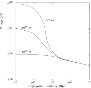
(32) 2.2. ULTRA-HIGH ENERGY COSMIC RAYS PHYSICS range between 5 · 1017 and the 3 · 1018 eV (the energies corresponding to the second knee and the ankle of the spectrum respectively, as will be explained later), all kind of nuclei, starting from protons up to Iron nuclei, are able to arrive from the local universe. On the other hand, the extragalactic magnetic fields are almost unknown but an upper limit of around 1 nG is usually accepted. An estimation of the deflection angle in a constant magnetic field which perpendicular component to the particle momentum is B⊥ over a distance d is given by [40]: µ o. θ(E, d) = 0.52 Z. E 20 10 eV. ¶−1 µ. B⊥ 10−9 G. ¶µ. d 1M pc. ¶ (2.2). In case of a proton of ∼ 1020 eV, the deviation is less than 1o in two scenarios: in the Galaxy where magnetic field is typically of ∼ µG on a distance ∼ kpc, or outside the Galaxy where the extragalactic magnetic field is the order of ∼ nG over a distance of the order of Mpc. The predicted cosmic ray deflections in the local supercluster are shown in Fig. 2.4(a), where values between 0 and 1◦ are found. As it can be seen in Eq. 2.2, higher the energy of the cosmic ray is, lower is the deflection (see Figure 2.4(b)), so that the door is opened to make cosmic ray astronomy at the highest energies. More detailed calculations could be found in [31, 41, 42].. Interactions of CRs during propagation and the GZK effect Unfortunately, propagation through galactic and extragalactic magnetic fields is not the only problem. Cosmic rays may interact with background radiation fields like the cosmic microwave background (CMB), the infrared background (IB) and radio background (RB), losing energy. Other energy losses are due to the Hubble expansion of the Universe and due to the interaction with dust, but they are not significant at the energies of our interest. The most important interaction at the highest energies is the GZK effect proposed by Greisen, Zatsepin, and Kuz’min [43, 44] just a bit later than the CMB discovery by Penzias and Wilson in 1965 [45]. They independently pointed out that this radiation would make the Universe opaque to cosmic rays of sufficiently high energy. Protons with an energy 16.

(33) CHAPTER 2. ULTRA-HIGH ENERGY COSMIC RAYS. Figure 2.5: Reduction of primary proton energy due to GZK effect. At 1022 eV particle would be reduced in energy to 1020 eV after traveling ∼ 100 Mpc (from [46]). exceeding E ∼ 5 · 1019 eV (called GZK threshold ) have a large probability to interact with the CMB photons, losing energy by pion photo-production: p + γCM B → p + Π0 → n + Π+. (2.3). These interactions occur via the ∆+ resonance whose cross section at that energy is very high (∼ 10−28 cm−2 ). Assuming typical value for the CMB photon density (400cm−3 ), the mean free path1 for a proton can be estimated as ∼ 8 Mpc. The energy loss per interaction for the proton is ∼ 20%, giving an attenuation length2 of the order of some tenths of Mpc, beyond which the proton energy falls below the GZK threshold. Fig. 2.5 shows how the energy of a proton degrades due to successive interactions with the CMB. On the other hand, the neutron decay length (n → p + e− + νe ) is about 1 Mpc at 1020 eV, so that it decays before interacting. If cosmic rays are protons, another energy loss process will be important between 1018 eV and the GZK threshold. It is the photo-pair production when protons interact with 1 2. The average distance covered by a particle between subsequent interactions The distance at which the probability that a particle has not been absorbed drops to 1/e. 17.

(34) 2.2. ULTRA-HIGH ENERGY COSMIC RAYS PHYSICS photons of the CMB producing a electron-positron pair (p + γCM B → p + e+ + e− ). The energy loss in each interaction is small. It may, however, contribute to the shape of the spectrum at these energies if the primaries are protons from distant sources. At lower energies the attenuation length tends to become constant and equal to the energy loss due to the expansion of the universe (∼ 4 Gpc). If cosmic rays are nuclei of mass A, they will undergo due to photo-disintegration and pair production, both with CMB and IR backgrounds: A + γCM B,IR → (A − 1) + N → (A − 2) + 2N → A + e+ + e−. (2.4). Since the energy is shared between nucleons, the threshold energy for these processes increases compared to that of protons. The inelasticity is lower by a factor ∼ 1/A, while the cross section increases with Z 2 . This means that the loss length, in case of heavy nuclei, will be smaller (∼ 1 Mpc) with respect to protons, but it occurs at a higher energies. Finally, if cosmic rays are photons, the dominant interaction is pair production with the cosmic background photons (γ + γCM B,RB → e+ + e− ). Pair creation with the CMB is important above 4·1014 eV while attenuation from pair creation with the radio background dominates the energy loss above 2 · 1019 eV. On the other hand, at energies higher than 1022 eV, the attenuation length grows to values of order of 100 Mpc, making possible the hypothesis of photons as primary of extremely-high energy cosmic rays. In fact, these photons could produce secondary photons at energies higher than the GZK-threshold. If this were the case, a secondary photon spectrum ∝ E −2 should be observed, independently on the source spectrum. Is charged particle astronomy possible? The interaction processes explained below are summarized in Fig. 2.6 and they have significant implications on the cosmic ray spectrum and on the possibility of making 18.

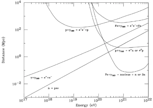
(35) CHAPTER 2. ULTRA-HIGH ENERGY COSMIC RAYS. Figure 2.6: Several interactions with the CMB. The curves labeled p+γCM B → e+ +e− +p and F e+γCM B → e+ +e− +F e are the distances for which the proton and the iron nucleus lose 1/e of their energy due to pair production. p + γCM B → N + π is the mean free path for photo-pion production. F e + γCM B → nucleus + n or 2n is the mean free path for spallation. γ + γCM B → e+ + e− is the mean free path for pair creation for photons with the CMB. n → p + e + ν is the mean decay length for a neutron. Figure from [47].. cosmic ray astronomy. First, due to the GZK effect, the observed spectrum should not extend, except at greatly reduced flux, beyond about several times 1019 eV. This expected suppression in the energy flux is known as the GZK suppression. Nevertheless, it does not mean that no event could be detected above this energy. In fact, some of them have been detected and are known as Super-GZK events. Second, Super-GZK events must have a nearby origin, cosmologically speaking, closer than one hundred of Mpc, usually called the GZK-sphere or the GZK-horizon. Otherwise, their energy would have been reduced below the GZK threshold due to this effect. Besides their interaction with cosmic photon backgrounds, charged particles are also affected by the presence of magnetic fields in the media they traverse. The intensity and 19.

(36) 2.2. ULTRA-HIGH ENERGY COSMIC RAYS PHYSICS topology of this fields is mostly unknown in the intergalactic medium but, if nG intensities are assumed, as a naive interpretation of Faraday rotation measurements would suggest, then protons at the highest energies could have gyroradii in excess of 100 Mpc. Therefore, charged cosmic rays originated at sources located at less that a few tens of Mpc, should keep enough directional information at Earth to produce observable anisotropy and make their astrophysical counterparts visible. The later opens the possibility of a charged particle astronomy in a similar sense as traditional photon-astronomy. At energies below few 1019 eV, the deflection due to the intergalactic and galactic magnetic fields combined is probably too large and only lower momenta of anisotropy can be expected even with very high statistics available. It is very likely that the same considerations apply, even at the highest energies, for nuclei heavier than protons. In any case, even for protons, only sources inside the GZK-sphere (. 100 Mpc) could be explored due to the combined effects of intervening radiation backgrounds and magnetic fields. It must be noted that some proposed exotic neutral particles, if they do exist, and neutrinos, if detected in enough quantities, may help probe a deeper portion of universe while keeping directional information.. 2.2.3. Energy and composition. The energy spectrum of cosmic rays is almost featureless. Extending from 109 up to 1020 eV, the spectrum follows a power law. dN (E) dE. ∝ E −α , where the index α is almost constant. and close to 3.0 in the whole energy range. The flux decreases 24 orders of magnitude along this energy range (Fig. 2.7). This behavior is expected in the case of stochastic acceleration of charged particles at astrophysical shocks as explained previously. The measured spectrum by the majority of the experiments is shown in Fig. 2.8. However, there exist some deviations from this power law fall-off at high energies. They are more clear in Fig. 2.9 where the flux is multiplied by E 2.7 . The first change is at ∼ 3 · 1015 eV and it is called the knee. A second possible steeping, the second knee, occurs at energies around ∼ 5·1017 eV. Another break where the spectrum turns up again, 20.

(37) CHAPTER 2. ULTRA-HIGH ENERGY COSMIC RAYS. Figure 2.7: Energy spectrum of cosmic rays. usually called the ankle, occurs at ∼ 3 · 1018 eV. The other key point is the highest energy region around and beyond the GZK-threshold. The spectral features might be interpreted as a change in the acceleration mechanism at the sources, as a propagation effect or as a change in composition or in the hadronic interaction processes involved. As can be seen in Fig. 2.9 several disagreements exist at the highest energies between different experiments: the normalization of the flux, the position of the ankle and the existence or not of the GZK suppression. We discuss these energy regions in detail in the following.. Galactic cosmic rays: the knee The knee, where the spectral index α increases significantly from 2.7 to about 3.1, is considered to be related with the limit of acceleration of lighter cosmic rays in the Galaxy. 21.

(38) 2.2. ULTRA-HIGH ENERGY COSMIC RAYS PHYSICS. Figure 2.8: The flux of cosmic rays as determined by the majority of the experiments. Vertical axis is multiplied by E 3 . Taken from [35].. Figure 2.9: The flux of UHECRs as determined by the several experiments. Vertical axis is multiplied by E 2.7 in order to make more visible the different features.. 22.

(39) CHAPTER 2. ULTRA-HIGH ENERGY COSMIC RAYS As it was shown in Eq. 2.1 the maximum acceleration is proportional to the atomic number of the element. In these models the energy achievable by nuclei is rigidity3 dependent. The knees of the spectrum of nuclei of charge Z are related to the proton knee energy p p Z Fe Eknee = ZEknee , where Eknee ' 3 · 1015 eV. Beyond the highest energy knee Eknee ∼ ·1017. eV, the total galactic flux, which is dominated by the Iron component, must be steeper. Possible acceleration sites are supernova remnants (SNR) [48]. It could be also related to the limitation of the galactic magnetic fields to bind the nuclei into the Galaxy when they reach these energies. Particles produced in SNR will be confined until a certain energy at which their Larmor radius becomes comparable to the size of the Galaxy. At this point particles will be able to leak out of the Galaxy producing a break in the spectrum that has been identified in the knee structure (details in [49]). This is assume as the standard scenario. However, other possibilities have been proposed. Another scenario assumes that the knee might be caused by a sudden change of the hadronic interactions at these energies [50]. In this case, the knee observed is not a characteristic of the spectrum itself, but of its observation at Earth. Finally, the knee can be interpreted also as a propagation effect due to a change in the regime of diffusion in the galactic magnetic field [51]. For a complete review about the observation and theoretical models for the interpretation of the knee see [52]. Transition region from galactic to extragalactic cosmic rays: from the knee to the ankle Assuming the standard scenario, the transition region from the galactic to extragalactic origin of cosmic rays occurs between the knee and the ankle. Thus, a drop of the heavy components at an energy scaled with the charge is expected. As commented before, if the knee is caused by light elements, another knee-like feature would be observed for the heaviest elements at higher energy. This is a possible explanation for the second knee where the spectrum steepens to α ∼ 3.3. This second knee should be in the region between 3. The rigidity is the momentum of the element over its charge.. 23.

(40) 2.2. ULTRA-HIGH ENERGY COSMIC RAYS PHYSICS 1017 to 1018 eV. It has been observed by the Fly’s Eye [53] and Akeno [54] experiments, but if it exists or not is still not clear. It is also being searched by KASCADE-Grande experiment [55]. The ankle, where the spectrum turns up with spectral index α ∼ 2.7, was first found by AGASA at 1019 eV [56], in agreement with Yakutsk [57]. However, it has been observed at around 3 · 1018 eV by Fly’s Eye [58], Haverah Park [59], Hires [30] and Auger [29]. Different interpretations of the transition region of the spectrum, between the knee and the ankle, have been proposed, with the consequent predictions on the cosmic rays composition. The standard interpretation for the ankle, called the ankle model (Fig. 2.10-left), is that the flat extragalactic component crosses the steep galactic spectrum, generating this feature at 1019 eV where the two components contribute equally to the total flux [60, 61]. The extragalactic component is thought to have a pure proton composition, so that the main problem in this model is how to explain a heavier composition up to 1019 eV. An alternative explanation is the dip model, recently proposed [62, 63] (Fig. 2.10right). It is build from the hypothesis that the extragalactic component, that is composed mainly of protons, starts to dominate at lower energies and the transition from the galactic to extragalactic CRs takes place at around 5 · 1017 eV (second knee), so that in the ankle region the galactic component has already vanished. The spectral index change in the ankle is just a propagation effect: protons passing through the cosmic microwave background loose energy via e− /e+ production and this causes a flux suppression at higher energies and an accumulation at a slightly lower energy. If composition above 1019 eV is not proton-like, another model called mixed composition model [64] is favored, because it assumes that extragalactic CRs have a mixed composition as the galactic component. As in the ankle model, the intersection of the galactic and extragalactic components gives origin to the the dip structure, but with the advantage of a lower transition energy at around E ∼ 3·1018 eV (Fig. 2.11), which softens the requirement of additional acceleration mechanisms and is more compatible with recent results by HiRes and Auger. The predicted spectrum and mass composition depends 24.

(41) CHAPTER 2. ULTRA-HIGH ENERGY COSMIC RAYS. Figure 2.10: Transition models: ankle model (left) and dip model (right). In the left panel, the extragalactic proton spectrum and the galactic component are shown, and the transition energy Etr is around 1019 eV . In the right panel, the extragalactic proton spectrum and the galactic component (dominated by Iron nuclei above EF e ) are shown, as well as the transition energy Etr that in this model is at the second knee. Data of KASCADE and HiResI, HiResII monocular spectra are shown. Taken from [35]. on several parameters (cosmological and describing the source composition), making the model very flexible and able to reproduce many composition profiles. The three models could be experimentally distinguished through accurate measurements of the spectrum, although the most discriminant feature is the chemical composition. Since in the ankle model the transition takes place at around 1019 eV, the galactic heavy component dominates up to the ankle energy. At higher energies the extragalactic component begins to dominate and the composition becomes proton dominated. Consequently, the composition in the dip region is dominated by heavy nuclei. On the contrary, in the dip model, as the transition is completed at energy around 1018 eV, the composition in the ankle region is proton dominated. The composition in the ankle region (Iron/proton) is a strong discriminant between both models. 25.

(42) 2.2. ULTRA-HIGH ENERGY COSMIC RAYS PHYSICS. Figure 2.11: The mixed composition model for the transition region of the spectrum under certain conditions. At E > 4 · 1019 the spectrum is characterized by GZK suppression. At energy 3 · 1018 eV the transition to pure extragalactic component is completed. HiResI, HiResII monocular spectra are shown. Taken from [35]. In the case of the mixed model, the transition between galactic and extragalactic (mixed composition) component occurs at 3 · 1018 eV . Consequently in the dip region the chemical composition is mixed, while at lower energies the Galactic heavy component dominates. This model predicts a slower decrease of the Iron component and a slower increase of the proton fraction in the transition energy range. At higher energies, due to photo-disintegration of the nuclei, the composition get lighter and at E > 3 · 1019 eV becomes strongly proton-dominated. A full discussion about the transition region could be seen at [65, 35].. The GZK suppression At higher energies, there were a controversy about the existence or not of the GZK suppression. AGASA reported a continuation of the cosmic ray flux in form of a power law [56], while HiRes observed a suppression above ∼ 5·1019 eV. Both use different techniques 26.

(43) CHAPTER 2. ULTRA-HIGH ENERGY COSMIC RAYS for detection and suffer a rapid increase with energy of the systematic uncertainties, mainly due to the lack of statistics. The dispute has been settled down by the recent results of the HiRes and Pierre Auger Observatory collaborations, where the flux suppression is determined with 5 and 6 standard deviations of significance respectively [30, 29]. Beyond the GZK The trans-GZK complex is affected by acceleration mechanisms, chemical composition of particles, cosmological evolution of the accelerating objects, and the existence of new physics. First, the theoretical upper limit is set by the product of the size of the objects and strength of the magnetic field in it, as shown in the Hillas diagram (Fig. 2.3). Therefore, if extreme energy particles are accelerated by the bottom-up processes in these known astronomical objects, it is highly likely that acceleration limit should be around 1020 eV, and a deep cut-off should exist in the energy spectrum. However, if the existence of the measured suppression is due to the GZK effect instead of a limit in the acceleration processes in the sources, it would exist a recovery in the spectrum around 3 · 1020 eV as a consequence of particles coming from sources closer to the GZK-horizon (see Fig. 2.12). In addition, in this scenario a bump would exist in the flux just at energies where the GZK begins, as a consequence of higher energetic particles that interact with the CMB photons and degrade their energy to that point (the cross section of this interaction is much lower below the GZK-threshold, see Fig. 2.6). Unfortunately, the discovery of the recovery would not solve this issue, because the recovery would also exists if the acceleration limit is still higher than the GZK energy. If this is the case, the existence of new categories of unknown objects located in the blank region at the upper right corner of the Hillas diagram is strongly suggested, otherwise, the top-down scenario must hold. Additionally, chemical composition of particles affects the shape of the trans-GZK complex, since it shifts in energy as the nucleus mass grows up. On the other hand, if we know the trans-GZK complex in detail, we could get some information on the chemical composition of the particles. If protons dominate and nucleus are negligible in 27.

(44) 2.2. ULTRA-HIGH ENERGY COSMIC RAYS PHYSICS. Figure 2.12: Theoretically predicted modification function of the spectrum of extreme energy particles due to the effect of propagation through the space. Here, m is a parameter that represents the degree of evolution of the sources. Taken from [66].. the chemical composition of the extreme energy particles, such a composition is difficult to be explained by the bottom-up scenario; it could be an evidence of the top-down scenario. If the nucleus component is comparable to solar abundance, it is the evidence of the acceleration in objects with standard chemical composition, such as galaxies including their nuclei. If nucleus components are more abundant compared to the solar abundance, it is the evidence of acceleration in metal-rich environment such as supernovae or gammaray bursts. Ground based experiments, such as Auger and Telescope Array, have major problems to perform the analysis described above, mainly because the observation area of such experiments is too small to get high enough statistics. The trans-GZK profile will be measured by the JEM-EUSO experiment (still in R&D phase), which achieves by far (700 times of AGASA) the large exposure required by observing from space [7]. 28.

(45) CHAPTER 2. ULTRA-HIGH ENERGY COSMIC RAYS The field of cosmic rays still represent a big challenge for physicists, both from theoretical and experimental point of view. Many people is working on this area (around 1000 papers were submitted to the International Cosmic Ray Conference that took place is Mexico in 2007), and important advances have been performed in last decade (see Section 3.5 where Auger results are shown). However, as it has been shown along this Section, most of the questions are only partially answered and the puzzle is still uncompleted.. 2.3 2.3.1. Extensive air showers Phenomenology. The flux of cosmic rays at energies higher than 100 TeV is so low that direct measurements are not useful. Fortunately, when a cosmic ray come into Earth, it interacts with a nucleus of the atmosphere, mainly Nitrogen or Oxygen, producing an extensive air shower (EAS). The first interaction is hadronic and usually takes place in the upper atmosphere (20-30 km depending on the energy and the mass of the primary). The particles can undergo due to all kind of nuclear reactions leading to the production of nuclear fragments and secondary particles. The primary energy is shared among these secondaries and, due to the enormous amount of energy available, they have a large probability to interact with other nuclei in the atmosphere and produce new particles before decaying into (mainly) photons, muons, electrons and neutrinos. Therefore, the secondary products again interact with the molecules of the atmosphere, emitting further secondary particles. In this way the particle multiplicity is increasing dramatically, leading to several million or billion of secondary particles which are heading towards the Earth’s surface with almost the speed of light. This cascade process is repeated until the energy of the secondary particles reaches the energy thresholds of the different processes involved. Then, the particles are absorbed, mainly by ionization, so the number of particles is reduced. To sum up, the number of particles increases, reaches a maximum at a certain depth in the atmosphere (called Xmax ), and decreases later. 29.

(46) 2.3. EXTENSIVE AIR SHOWERS The theory of electromagnetic interactions is assumed to be still valid at these energies, but the hadronic interactions are more problematic because they require far extrapolations of empirical models tuned on experimental data at lower energy. In fact, data from accelerators is used but the energetic range studied is limited; the center of mass energy √ √ in a nucleon-nucleon collision is given by s ∼ 2mn E. For example, the energetic limit foreseen for LHC (∼ 14 TeV) corresponds to a nucleon energy of 1017 eV . The needed extrapolations induce uncertainties on the first steps of the cascade, which cannot be directly observed. Nevertheless, simple models describing the development of the showers exist. The toy model suggested by Heitler [67] provides the macroscopic characteristics of an electromagnetic showers, while the development of hadronic showers induced by protons could be described by a similar model [68]. Even if they cannot replace detailed simulations, these simple models predict the most important features of the cascades. The nucleus-air interactions could be described by applying the superposition model. Assuming that the incoming projectile is a nucleon or a nucleus with atomic number A (in practice A ≤ 56, because nuclei heavier than iron are not abundant), the primary interaction is hadronic and, as a first approximation, a nucleus A of energy E is equivalent to the superposition of A independent nucleons each with energy E/A (the binding energy of nucleons is ∼ 8 MeV, consequently at high energies they can be considered as free nucleons). In Fig. 2.13-left a sketch of the different components of an extensive air shower is shown and the energy flow between different air shower components is in Fig. 2.13-right. In more detail, the different interactions involved are explained next. The primary interaction produces a large number of secondaries, mainly pions (π 0 , π + , π − ) and kaons (K + , K − ), which give rise to further hadronic interactions, and so on: this is the hadronic cascade. This component of the shower is also fed, in a low fraction, by the photons via two pion photo-production processes (γ + γ → π + + π − ) in the presence of a nucleus and the muon when collides with a nucleon. The lifetime of neutral pions is τ0 = 8.4 · 10−17 s, so that they immediately decay into photons before interacting. 30.

(47) CHAPTER 2. ULTRA-HIGH ENERGY COSMIC RAYS. Figure 2.13: Left: Sketch of the different components in an extensive air shower. Right: Energy flow between different air shower components. The thickness of the arrows illustrates the amount of energy transferred in the given direction by the stated processes (from [69]). Therefore, at each step of the hadronic cascade, about 1/3 of the energy is transferred to photons, giving raise to the electromagnetic cascade: π 0 → γ + γ (∼ 98.8%). (2.5). π 0 → e+ + e− + γ (∼ 1.2%). (2.6). where the branching ratios of the two decay channels are given in the brackets. The hadronic cascade ends up with the decay of charged pions into muons (as will be shown later), at intermediate altitudes around 6 km with large spread. Therefore, only few nucleons, pions, kaons and nuclear fragments (the hadronic cascade) reach the ground and very colimated with shower axis. Photons produce e+ /e− pairs and Compton electrons, and electrons/positrons radiate through bremsstrahlung on atmospheric nuclei which leads to the emission of further 31.

(48) 2.3. EXTENSIVE AIR SHOWERS photons, which afterwards again may produce additional e+ /e− pairs, and so on: γ + N → N + e+ + e− e± + N → N + e± + γ. (2.7) (2.8). This chain reaction proceeds until the energy of the electrons and positrons drops below the critical energy4 , which is around 85 MeV in air. Then, the ionization energy loss starts to dominate the Bremsstrahlung process. Pure electromagnetic cascades can also be initiated directly by high energy photons or electrons. A small fraction of the electromagnetic component is re-injected in the hadronic cascade because of hadronic interactions of the photons as shown below. As consequence, a shower induced by a primary photon would also develop an hadronic cascade. The decay of secondary pions and kaons generate neutrinos and the muon component via: π ± → µ± + νµ (νµ ) (∼ 99.99%) (τ0 = 2.6 · 10−8 s). (2.9). K ± → µ± + νµ (νµ ) (∼ 63.54%) (τ0 = 1.2 · 10−8 s). (2.10). K ± → π ± + π 0 (∼ 20.68%). (2.11). The muons are produced with typical energy of few GeV, increasing with the altitude of production. In addition, they inherit the transverse momentum of their parents (a few hundred of MeV), so their divergence5 is relatively small and strongly anti-correlated to their energy (more energetic muons are close to shower axis). Few muons are also produced via the electromagnetic interactions of photons (γ + γ → µ+ + µ− ). A large fraction of muons reach the ground before decaying, with a non-negligible energy loss (' 2M eV /(gcm−2 )). Muons, however, may decay in flight when their energy drops below 10 GeV, producing a second source of neutrinos and e+ /e− : µ± → e± + νe (νe ) + νµ (νµ ) (∼ 99%) 4. (2.12). The critical energy Ec for the electrons is defined as the energy at which the loss by ionization (∝ Z). equals the loss by radiation (∝ Z 2 ). Ec ∝ 1/Z 5 the angle respect to the shower axis. 32.