Modeling the Effects of Exercise on Blood Glucose Concentration Level and their Compensation with the Design of a Feedforward Predictive Control Strategy-Edición Única

Modeling the Effects of Exercise on Blood Glucose

Concentration Level and their Compensation with the Design of

a Feedforward Predictive Control Strategy-Edición Única

Title

Modeling the Effects of Exercise on Blood Glucose

Concentration Level and their Compensation with the

Design of a Feedforward Predictive Control

Strategy-Edición Única

Authors

León Cantú García

Affiliation

Tecnológico de Monterrey, Campus Monterrey

Issue Date

2009-12-01

Item type

Tesis

Rights

Open Access

Downloaded

18-Jan-2017 15:52:36

INSTITUTO TECNOLÓGICO Y DE ESTUDIOS 

SUPERIORES DE MONTERREY 

CAMPUS MONTERREY 

G RA D U A T E PRO G RA M IN M ECHA TRO N ICS A N D

IN FO RM A TIO N TECHN O LO G IES

M ODELING THE EFFECTS OF EXERCISE O N BLOOD GLUCOSE CONCENTRATION LEVEL AND THEIR U>MFKNSAT10N WITH THE

DESIGN OF A FEEDFORWARD PREDICTIVE CONTROL STRATEGY

PRESEN TED A S A PA RTIA L FULFILLM EN T O F T H E

REQ UIREM EN TS FOR T H E D EG REE O F

M A STER O F SCIEN CE W ITH M AJOR IN A U TO M A TIO N

TECNOLÓGICO 

DE MONTERREY 

THESIS

BY 

LEÓN CA N TÚ GA RCIA

INSTITUTO TECNOLÓGICO Y DE ESTUDIOS 

SUPERIORES DE MONTERREY 

M O N TERREY  CA M P U S 

GRA D U A TE  P RO G RA M  IN  M ECH A TRO N I CS  A N D 

I N FO RM A TI O N TECH N OLOGI ES 

TECNOLÓGICO 

DE M ONTERREY 

MODELING THE EFFECTS OF EXERCISE ON BLOOD GLUCOSE 

CONCENTRATION LEVEL AND THEIR COMPENSATION WITH THE 

DESIGN OF A FEEDFORWARD PREDICTIVE CONTROL STRATEGY 

THESIS 

PRESEN TED  A S A PARTI AL FU LFI LLM EN T OF THE  REQ U I REM EN TS 

FOR THE DEGREE OF 

M A STER OF SCIEN CE W I TH  M A JO R IN  A U T O M A T I O N 

BY 

LEÓN CANTÚ GARCÍA 

MODELING THE EFFECTS OF EXERCISE ON BLOOD GLUCOSE 

CONCENTRATION LEVEL AND THEIR COMPENSATION WITH THE 

DESIGN OF A FEEDFORWARD PREDICTIVE CONTROL STRATEGY 

BY 

LEÓN CANTÚ GARCÍA 

THESIS 

PRESENTED TO THE GRADUATE PROGRAM  IN M ECHATRONICS AND 

INFORM ATION TECHNOLOGIES 

THIS THESIS IS A PARTIAL REQUIREM ENT FOR THE DEGREE 

OF M ASTER OF SCIENCE WITH MAJOR IN 

AUTOM ATION 

INSTITUTO TECNOLÓGICO Y DE ESTUDIOS 

SUPERIORES DE MONTERREY 

M ONTERREY CAM PUS 

INSTITUTO TECNOLÓGICO Y DE ESTUDIOS 

SUPERIORES DE MONTERREY 

M ONTERREY CAM PUS 

GRADUATE PROGRAM  IN M ECHATRONICS AND 

INFORM ATION TECHNOLOGIES 

The members of the thesis committee hereby approve the thesis of Leon Cantu Garcia  as a partial fulfillment of the requirements for the degree of M aster of Science with 

major in  Automation 

To God, for standing always by my side. 

To M irtala and Francisco, for being my greatest support. 

To Ismael, for sharing his medical knowledge. 

To Celina, for her company and love. 

To AECR, for being an unconditional friend. 

For the Town boys, for making the stress to go away. 

To myself. 

Table of contents 

Abstract....,zyxwvutsrqponmlkjihgfedcbaZYXWVUTSRQPONMLKJIHGFEDCBA I 

Chapter 1 1  Introduction 1  1.1. Justification 2  1.2. Problem Statement 2  1.3. Objectives 2  1.4. Contents description 3  Chapter 2 4  Background 4  2.1. Biological sciences 4  2.1.1. Endocrinology basis 4  2.1.2. Glucose and its metabolism 5 

2.1.2.1. Glucose structure 5 

2.1.2.2. Glycolysis 6 

2.1.3. Glucose regulation via insulin and glucagon hormones 11 

2.1.3.1. Insulin effects 11 

2.1.3.2. Glucagon effects 12 

2.1.4. Diabetes M ellitus 12  2.1.5. Homeostasis changes during exercise 14 

2.1.5.1. Effects on Heart Rate 14 

2.1.5.2. Effects on Oxygen Uptake 14 

2.1.5.3. Effects on Blood Flow 14 

2.1.5.4. Effects on glucose and insulin plasma levels 15  2.2. Systems Identification and Control Theory 16  2.2.1. Systems Identification and M odeling 16 

Chapter 3 20  State of the art 20 

3.1. Glucose model development 20 

3.1.1. Ackerman's model 20 

3.1.2. Sorensen's model 22 

3.1.2.1. Sorensen's base model 22  3.1.2.2. Sorensen's model with the addition of exercise as a disturbance 23  3.1.3. Bergman's model 28  3.1.3.1. Bergman's base model 28  3.1.3.2. Bergman's base model with the addition of exercise as a disturbance 30  3.2. Glucose control strategies 35 

3.2.1. Feedback strategy 36 

3.2.1.1. Definition 36  3.2.1.2. Application to glucose­insulin system 36 

3.2.2. Feedforward strategy 36 

3.2.2.1. Definition 36  3.2.2.2. Disturbance modeling applied to the glucose ­ insulin system 36 

3.2.3. Adaptive control strategy 39 

3.2.3.1. Definition 39  3.2.3.2. Application to glucose­insulin system 39 

3.2.4. Robust control strategy 40 

3.2.4.1. Definition 40  3.2.4.2. Application to glucose­insulin system 41 

3.2.5. Optimal control strategy 41 

4.1.1. M odification in Sorensen's model 45 

4.1.2. Simulation of modified Sorensen's model 48 

4.1.3. Simulation of the Bergman minimal order model 57 

4.1.4. Combination of Bergman's and Sorensen's model 60 

Chapter 5 65  Experiment design for statistical modeling 65  5.1. Criterion of the statistical experiment design 65  5.2. Data used in glucose system experiment 67  5.3. Data obtained in the experiment 70  Chapter 6 72  Statistical modeling 72  6.1. Hammerstein ­ Wiener modeling technique 72 

6.1.1. Definition 72 

6.1.2. System identification via Wiener technique 73 

6.1.3. Wiener modeling advantages over other modeling methods 75 

6.1.4. Wiener modeling applied to glucose regulation 76 

6.1.4.1. Development of the Wiener model without normalization of data 77  6.1.4.2. Development of the Wiener model with normalized data (N(u=0,cr2=l)) 80  6.1.4.3. Development of the Wiener model with scaling of each input with respect to its maximum value and  a sample time of 10 minutes 84  6.1.4.4. Development of the Wiener model with scaling of each input by dividing by its maximum value and a  sample time of 5 minutes 88  6.1.4.5. M odifications in the chosen predictive model 91  6.1.4.6. Testing phase of the predictive model 94  Chapter 7 98  Predictive controller design 98  7.1. M odel based predictive control strategy applied to glucose level regulation 98  7.2. Physical implementation of the feedforward predictive compensator 116 

7.2.1. Disturbance measurement and sensor technology 117 

7.2.2. Actuator and reservoir 118 

8.1. Discussion of results 119  8.1.1. Results from analytical modeling 119 

8.1.2. Results from statistical modeling 120  8.1.3. Results from the predictive control implementation 121 

8.2. Conclusions and future challenges 124 

8.2.1. Conclusions 124  8.2.2. Future challenges 124 

List of tables 

Table I. Comparison between aerobic and anaerobic glycolysis 6  Table II. Comparison between Diabetes Type I and Type II 13 

List of figures 

Figure 1. Linear and Hemiacet al ring D-Glucose st ruct ureszyxwvutsrqponmlkjihgfedcbaZYXWVUTSRQPONMLKJIHGFEDCBA 6 

Figure 2. Food t o energy pat h 7 

Figure 3. Glycolysis react ions. Taken from Albert s 9 

Figure 4. Krebs Cycle. Taken from ht t p:/ / en.w ikipedia.Org/ w iki/ File:Cit riccycle.svg 10 

Figure 5. Oxidat ive phosporylat ion process. Taken from Albert s 11 

Figure 6. St at ist ical ident ificat ion of a syst em 16 

Figure 7. Block diagram of st at ist ical modeling 17 

Figure 8. Cont rol syst em block diagram. R(t ) is t he reference signal, 19 

Figure 9. Compart ment s in Sorensen's m odel 22 

Figure 10. Peripheral glucose upt ake by exercising muscle. Solid line is t he predict ion 25  Figure 11. Glucose response t o a 30% PV02max st ep. Dot t ed line represent s 27  Figure 12. Glucose response t o a 60% PV02max st ep. Dot t ed line represent s 27 

Figure 13. Sorensen's m odel adding t he effect of exercise 28  Figure 14. Bergman's minimal order m odel of glucose-insulin int eract ion 29 

Figure 15. Dependence of glycogen deplet ion commencement t ime, tgiyon exercise int ensit y u3(t ) 32 

Figure 16. Glucose (Top) dynamics due t o exercise at int ensit y of 30% PV02max, 34 

Figure 17. Glucose dynamics due t o exercise at int ensit y of 60% PVOlmax, 34 

Figure 18. Block diagram of glucose - insulin cont rol syst em 35 

Figure 20. Glucose response predict ion due t o different input s using H-W 37 

Figure 19. Block diagram of Feedforw ard st rat egy. 37 

Figure 21. Glucose response predict ion due t o different input s. Using H-W met hod on a five days t rial.. 38 

Figure 22. Glucose response predict ion due t o different input s. Using H-W met hod on 38 

Figure 23. Block diagram of adapt ive cont rol st rat egy. 39 

Figure 24. Result s of glucose regulat ion using Run t o run st rat egy. 40 

Figure 25. Schemat ic of a syst em 's m odel, Gt(s), w it h paramet ers uncert aint y addit ion 41 

Figure 26. Block diagram of closed loop syst em for t he regulat ion of 42  Figure 27. Glucose regulat ion using an opt imal cont rol st rat egy, w it h 43  Figure 28. Plasma glucose and insulin responses, using an int elligent 44  Figure 29. Schemat ic of t he implement at ion of t he global Sorensen's m odel. 49 

Figure 30. Schemat ic of t he compart ment s in Sorensen's m odel. Red lines limit glucose compart ment s; 49 

Figure 31. Schemat ic of exercise effect s in Sorensen's m odel: pancreat ic glucose upt ake and 50  Figure 32. Dynamic response of%PV02

ma

* (blue) and 25% PAM M input (red) 50  Figure 33. Dynamic response ofPGUa (blue) w it h 25% PAM M or 30% PV02

m ox

. 51 

Figure 34. Dynamic response of net HGPa (blue) w it h 25% PAM M or 30% PVOi™" 51 

Figure 35. Dynamic responses of blood flow s (L/ m in) for insulin t ransport in t he 52  Figure 36. Dynamic responses of blood flow s (dL/ m in)for glucose t ransport in t he 52  Figure 37. Dynamic responses of glucose (green) (m g/ dL) and insulin (red) (m U/ L) 53  Figure 38. Dynamic response of%PV02

max

Figure 39. Dynamic response ofPGU„ (blue) w it h 59.1% PAM M or 60% PV02 m a

* .zyxwvutsrqponmlkjihgfedcbaZYXWVUTSRQPONMLKJIHGFEDCBA 54 

Figure 40. Dynamic response of net HGPa (blue) w it h 59.1% PAM M or 60% PV02 m m

. 55 

Figure 41. Dynamic responses of blood flow s (L/ m in)for insulin convect ive t ransport . 55  Figure 42. Dynamic responses of blood flow s (dL/ m in)for glucose convect ive t ransport . 56  Figure 43. Dynamic responses of glucose (green (m g/ dL)) and insulin (red) (m U/ L) 56 

Figure 44. Global schemat ic of t he implement at ion of Bergman 57  Figure 45. Compart ment s X (remot e insulin), I (art erial insulin) and 58  Figure 46. Schemat ic of t he compart ment s w here PV02

m ax

, PGUg, and net HGPa are calculat ed. 58 

Figure 47. Response of glucose (blue)(m g/ dL) and insulin (pU/ m L) art erial concent rat ion w it h an 59  Figure 48. Response of glucose (blue)(m g/ dL) and insulin (pU/ m L) art erial concent rat ion w it h an 60 

Figure 49. Schemat ic of t he implement at ion of hepat ic glucose product ion 62 

Figure 50. Schemat ic of t he combinat ion of Sorensen's and 63 

Figure 51. Response of glucose level (blue) (m g/ dL) t o ext ernal glucagon infusion rat e st ep (green) (104

pg/ m in) 63 

Figure 52. Glucose rat e of change (m g/ dL/ m in) response t o a pulse input of 30 PAM M (%)from 67 

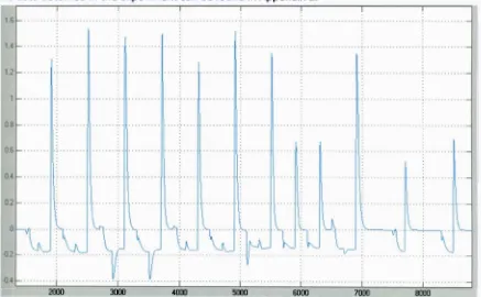
Figure 53. Dat a obt ained in t he experiment : Glucose concent rat ion (blue) (m g/ dL) response t o 70 

Figure 54. Dat a obt ained in t he experiment : Glucose rat e of change (blue) (m g/ dL/ m in) 71 

Figure 55. Block diagram of W iener syst em for one out put t ]h 73 

Figure 56. Performance of t he syst em in t he t raining and t est ing phases 76 

Figure 57. Comparison bet w een t he predict ed nonlinear st eady st at e glucose concent rat ion 78 

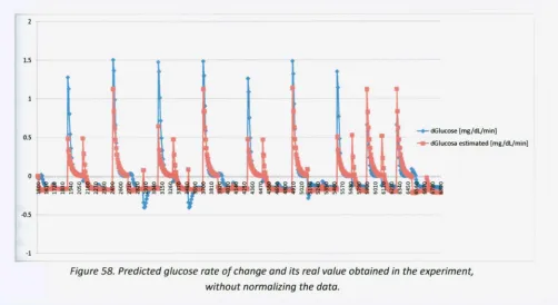
Figure 58. Predict ed glucose rat e of change and it s real value obt ained in t he experiment , 80 

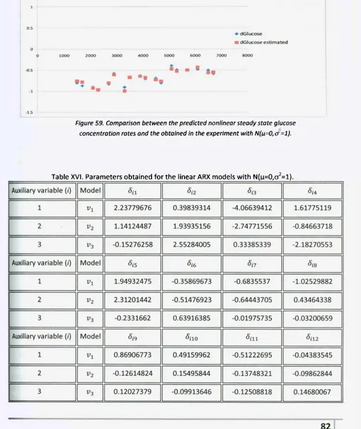
Figure 59. Comparison bet w een t he predict ed nonlinear st eady st at e glucose 82 

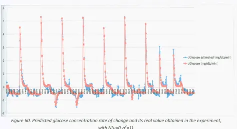
Figure 60. Predict ed glucose concent rat ion rat e of change and it s real value obt ained in t he experiment ,

84 

Figure 61. Comparison bet w een t he predict ed nonlinear st eady st at e glucose concent rat ion rat es 86  Figure 62. Predict ed glucose rat e of change and it s real value obt ained in t he experiment , 88  Figure 63. Comparison bet w een t he predict ed nonlinear st eady st at e glucose concent rat ion rat es 90  Figure 64. Predict ed glucose concent rat ion rat e of change and it s real value obt ained in t he experiment ,

91 

Figure 65. Predict ed glucose concent rat ion rat e of change and it s real value obt ained in t he experiment ,

92 

Figure 66. Comparison bet w een t he predict ed and real glucose concent rat ion rat e in t rial #1 95  Figure 67. Comparison bet w een t he predict ed and real glucose concent rat ion rat e in t rial #2 95  Figure 68. Comparison bet w een t he predict ed and real glucose concent rat ion rat e rat e in t rial #3 96  Figure 69. Comparison bet w een t he predict ed and real glucose concent rat ion rat e in t rial #4 96  Figure 70. Comparison bet w een t he predict ed and real glucose concent rat ion rat e in t rial #5 97 

Figure 71. Comparison bet w een t he predict ed and real glucose concent rat ion rat e in t rial #6 97 

Figure 72. Response of glucose level (m g/ dL) (blue) in close loop, w it h 99 

Figure 73. Flow chart of t he predict ive cont rol algorit hm for exercise effect s compensat ion 101 

Figure 75. Implement at ion schemat ic of complet e aut omat ic syst em w it h predict ive cont rol st rat egy for

Figure 74. Block diagram of complet e glucose level cont rol syst em w it h compensat ion of exercise effect s

102 

Figure 76. Performance of predict ive cont rol st rat egy, w it h 10% PAM M (blue) and 105 

Figure 77. Performance of predict ive cont rol st rat egy, w it h 15% PAM M (blue) and 105 

Figure 78. Performance of predict ive cont rol st rat egy, w it h 20% PAM M (blue) and 106 

Figure 79. Performance of predict ive cont rol st rat egy, w it h 25% PAM M (blue) and 106 

Figure 80. Performance of predict ive cont rol st rat egy, w it h 30% PAM M (blue) and 107 

Figure 81. Performance of predict ive cont rol st rat egy, w it h 35% PAM M (blue) and 107 

Figure 82. Performance of predict ive cont rol st rat egy, w it h 40% PAM M (blue) and 108 

Figure 83. Performance of predict ive cont rol st rat egy, w it h 40% PAM M (blue) and 108 

Figure 84. Performance of predict ive cont rol st rat egy, w it h 10% PAM M (blue) and 109 

Figure 85. Performance of predict ive cont rol st rat egy, w it h 30% PAM M (blue) and 109 

Figure 86. Performance of predict ive cont rol st rat egy, w it h 40% PAM M (blue) and 110 

Figure 87. Performance of predict ive cont rol st rat egy, w it h 10% PAM M (blue) and 110  Figure 88. Performance of predict ive cont rol st rat egy, w it h 30% PAM M (blue) and  I l l  Figure 89. Performance of predict ive cont rol st rat egy, w it h 40% PAM M (blue) and  I l l  Figure 90. Performance of predict ive cont rol st rat egy, w it h 10% PAM M (blue) and 112  Figure 91. Performance of glucose level w hen m eal and exercise dist urbance excit e t he syst em 113 

Figure 92. M anipulat ed variables of t he feedback PID cont roller (ext ernal insulin in mU/ min)(green) and

feedforw ard predict ive compensat or (ext ernal glucagon in pg/ m in)((blue) 114  Figure 93. Response of blood glucose level w hen m eal and exercise dist urbance excit e t he syst em in

manual mode 115 

Figure 94. Performance of predict ive cont rol st rat egy. W it h 40% PAM M (blue) and a durat ion of 150 minut es. Glucose st eady st at e level at 90 mg/ dL(cyan).GIucose concent rat ion response in red. Insulin

concent rat ion level in green 121 

Figure 95. Performance of predict ive cont rol st rat egy. W it h 45% PAM M (blue) and a durat ion of 100 minut es. Glucose st eady st at e level at 90 mg/ dl(cyan).Glucose concent rat ion response in red. Insulin

concent rat ion level in green 122 

Figure 96. Performance of predict ive cont rol st rat egy. W it h 40% PAM M (blue) and a durat ion of 200 minut es. Glucose st eady st at e level at 90 mg/ dL(cyan).GIucose concent rat ion response in red. Insulin

concent rat ion level in green 122 

Chapter 2 

Background 

2.1. Biological sciences 

2.1.1.

 Endocrinology basis 

As it can be seen, this path has a huge importance since it allows feedback (negative or positive) of  the current hormone level. In medical terms, a positive feedback means incrementing the release of a  hormone, and a negative feedback, decreasing it. This control mechanism impedes an unbalance of  hormones in the body, due to a large or a low  concentrations of them, that can provoke diseases like the  Cushing Syndrome. The main reason of failure in this path is when a tumor arises in any of its elements.  It is important to remark the action mechanism and effects of the hormone released by a glandule in  the target organ. The hormone anchors in specific receptors located in the cell membrane or in the  nucleus and produces a desired reaction. If the receptors that detect the hormone are in the membrane,  they generate a series of events, called second messengers, inside the cell, but if they are in the nucleus,  their action consists on a modification of the DNA. 

2.1.2.

 Glucose and its metabolism 

Figure 1. Linear and Hemiacet al ring D-Glucose st ruct ures. 2.1.2.2. Glycolysis  Metabolism is defined as the chemical reactions that occur in the body in order to obtain energy  (Guyton &  Hall, 2001). It can be divided in two major parts: catabolism and anabolism. The first one is  the process of converting complex macromolecules into simple molecules; anabolism designates the  reactions that make a macromolecule from simple elements.  Glycolysis is the metabolism of glucose. Depending on the organism and the cells specialization, there  can be two types of glycolysis, which are aerobic and anaerobic. The usage of depends on the  cardiovascular system's capacity of satisfying the oxygen and glucose uptake demands by the muscles  (Alberts, 2002).  Pasteur classified the cells in charge of oxidizing glucose in three categories: strict aerobe cells that  form C02 and H20; anaerobe strict cells that form lactic acid and facultative anaerobe cells that behaves 

as either of the other two types of cells (M urray, 1993).  Table I. Comparison between aerobic and anaerobic glycolysis.  The conversion of glucose into energy has several biochemical steps that occur in the cells  mitochondria, and takes different paths depending on the type of glycolysis.  The first step is transforming glucose into pyruvate, in medical terms this is known as glycolysis. It is  important to acknowledge that aerobic and anaerobic glycolysis follow  these same reactions and the  total gain of this phase is 4 adenosine triphosphate (ATP) and 2 nicotinamide adenine dinucleotide  (NADH) molecules; the second step is called Kreb's cycle or Citric acid cycle, which has the function of  capturing H*  from the different reactions that happen inside the mitochondria; the third step has the  main goal of generating ATPs from the hydrogen obtained in the NADH and FADH2 molecules via the two 

Figure 3. Glycolysis react ions. Taken from Albert s (202).

After glycolysis process ends, the next biochemical reactions that occur in the organism are known as  the Krebs cycle. 

This energy generation process occurs inside the mitochondria, and it has a net gain of 3 NADH, 1  FADH2 and 1 ATP. Its main purpose is not the production of ATP but the attainment of hydrogen atoms.  Citric acid cycle is divided in eight principal reactions (Alberts, 2002): 

1) Conversion of acetyl CoA to citrate. The acetyl CoA combines with an oxaloacetate molecule and  via the citrate synthase enzyme to form citrate. 

3) Oxidation of isocitrate. In this reaction the first NADH is generated by the oxidation of isoscitrate  to ot­ketoglutarate.  4) Conversion of a­ketoglutarate to succinyl­CoA. The first decarboxylation occurs and another  NADH is obtained.  5) Transformation of succinyl­CoA to succinate. The only ATP gain occurs.  6) Oxidation of succinate. Succinate­dehydrogenase enzyme oxidizes succinate molecule, in order  to obtain Fumarate and FADH2  7) Transformation of fumarate to L­malate. Fumarate is hydrated and generates L­malate.  8) Oxidation of L­malate to oxaloacetate. This final step generates the final NADH molecule.  The reaction in this cycle can be summarized as: 

Acetyl CoA + 3 NAD + FAD + ADP + Pi +2 H20 ­» 2 C02 + 3 NADH + 3 H + FADH2 +ATP + CoA 

Figure 4. Krebs Cycle. Taken from ht t p:/ / en.w ikipedia.Org/ w iki/ File:Cit riccycle.svg

Finally, the last  group of reactions is known as oxidative phosphorylation, which is the most  important step. 

This process synthesizes ATP when electrons from NADH and FADH2 are transferred to  02 in the  mitochondria's matrix. The total energy generation is in the order of 3 ATP /  1 NADH and 2 ATP /  1  FADH2. 

The summary of this process is (Alberts, 2002): 

4) For an ATP bomb can be used, the complex ADP + Pi (phosphate) must link t o it . After the  process is done, H+

 returns to the mitochondria's matrix and a new product is formed, ATP. 

Figure 5. Oxidat ive phosporylat ion process. Taken from Albert s (2002).

As it has been seen, conversion from food to energy is a very complex process, which involves a lot of  reactions, but all of them can be regulated depending on the body's needs using enzymes. 

2.1.3. Glucose regulation via insulin and glucagon hormones 

According to Guyton (2001), the normal glycemic range in the plasma is 60 ­ 110 mg/ dL. When the  level drops or is increases beyond these values, the patient starts to feel illness, presenting symptoms,  like lack of energy, paleness, headache, among others. It  is in this situation when the endocrinology  system starts its control with the goal of keeping glucose in the desired range. The two hormones  involved in glycemic regulation are insulin and glucagon. 

2.1.3.1. Insulin effects 

ozyxwvutsrqponmlkjihgfedcbaZYXWVUTSRQPONMLKJIHGFEDCBA Dehydration. It occurs due to an increase of the osmotic pressure in the extracellular  compartment, provoking water to flow  outside the cell.  o Tissue lesion. A chronic hyperglycemic level will have a negative impact in the blood vessels,  causing a morphological change in them and poor irrigation of several organs. This syndrome will  increment the possibility of myocardial infarction, ictus, lethal renal diseases, retina injure,  blindness and limbs gangrene.  o Usage of fat and protein as energy. The alteration of the carbohydrate metabolism will induced  the usage of fat to satisfy the energy uptake demand. Nevertheless, the production of keto acids  is greater than its consumption, this will provoke a metabolism acidosis that can take the patient  to a diabetic coma. Also protein will be used for energy considerations, causing dystrophy in the  organism tissues.  •  Type II, also known as non­insulin dependence diabetes or insulin resistance.  In this kind of diabetes, there is insulin production but the cells sensitivity to this hormone is very  low. As in type I, metabolism of carbohydrates, fats and proteins metabolism is altered, and  symptoms are almost the same except for the high production of keto acids.  This is the most common type of Diabetes mellitus, since it includes 90% of this disease cases and it  usually starts at the age of 50 (Guyton &  Hall, 2001).  Type II Diabetes effects (Guyton &  Hall, 2001):  o Increase of plasmatic insulin. Due to a lack of sensitivity in the insulin receptors, glycaemic level  increments, this situation makes the 3­Langerhans cells produce more of this hormone in order  to lower the glucose level, but the response will not be the desired one because of receptors  resistance to insulin. 

o Obesity. There are two theories of how  obesity and diabetes are related. One indicates that  obese people have less insulin receptors in the muscles, liver and adipose tissue. The other  expresses that there is an alteration in the activation signals on the insulin receptors. 

Depending on the type of diabetes the patient has, there are several treatments to follow. If it is type  I, the only remedy is the external insulin shot, which is classified in two forms: the regular injection, for a  basal one­day­long effect, and the supplementary injection, that is taken before a meal.  For type II, exercise and diet are the first treatment. According to Kronenberg (2002), exercise will  increment insulin sensitivity in the cells, and glycemic level will decrease as consequence. If this fails,  insulin shots have to be taken (Guyton &  Hall, 2001) 

2.1.5. Homeostasis changes during exercise 

2001; Firman 2005). Although these changes are beneficial to the organism because it improves the  quality of life of people, if a patient has an illness, like Diabetes M ellitus, exercising at a high intensity or  for a long time can provoke serious issues to his health.  2.1.5.1. Effects on Heart Rate  According to Firman (2005), the heart rate in an adult person is approximately 78 heart beats/ min,  but if a person is exercising, it will raise up to 200 heart beats /  min, depending on the duration and  intensity of the exercise.  Firman showed evidence that HR has a direct relation with oxygen uptake, that depends on the  active muscles demand. Firstly there is not enough quantity to satisfy the needs, so a chemical  stimulation is induced in order to increase the HR; as a second stage, the increment of the HR will also  increase the heart and blood flow, allowing faster oxygen transportation to the active muscles.  2.1.5.2. Effects on Oxygen Uptake 

In an adult person, the normal oxygen uptake is 250 mL/ min, but it can rise up to 5100 mL/ min,  depending on the physical resistance. Additionally, this measure can vary due to the person's gender  and age. Therefore, it is preferable to handle a percentage of maximum oxygen uptake ratio (PV02 m ax  or zyxwvutsrqponmlkjihgfedcbaZYXWVUTSRQPONMLKJIHGFEDCBA V02 m sx ), in order to make comparisons among people.  Fehlig and Wahren (1975) reported that PV02 m a x

 has a basal value of is 8% and takes approximately  from 4 to 5 minutes to reach its maximum. 

In basal conditions, the skeletal muscle only receives 15% of the total heart flow ; also the arterioles that  irrigate those muscles are closed. However, when exercise begins, the following reactions occur (Firman,  2005):  1. At the beginning of the exercise, as it was explained, heart rate and heart flow  increase; this  situation induces a reaction in the sympathetic nervous system that will open the arterioles in  the skeletal muscles and close the ones in the abdominal region and skin, this is done with the  purpose of pumping more blood to the active muscles.  2. The increase of metabolism waste products of skeletal muscles acts as a direct signal in the  nervous system, so arteries nearby can dilate, allowing active muscles to receive the blood flow   from other zones of the organism; the arterioles from those regions will be closed due to a  signal sent by the sympathetic nervous system. 

With the knowledge of these effects. Chapman &  M itchell (1965) realized a research pointing out the  variations of blood flow  in the organs during exercise. It is indispensable to remark that all of these  changes are consequences of the active muscular mass, and this one is linked directly to an increase in  PV02 m ax ; according to Andersen et al. (1985), this means that blood flow  in active muscles is a linear  function of exercise intensity. 

Table III. Relationship between blood flow  (dL/ min) in organs and exercise intensity (%). 

2.2. Systems Identification and Control Theory 

2.2.1.

 Systems Identification and M odeling 

According to Ogata (2002), a system is defined as a combination of components that act together  and perform a certain objective. In order to fully comprehend any system found in nature, it is necessary  to understand and represent how  it responds to a known input variable or several inputs. This concept is  known as system modeling.  The process of modeling a system can be done in an analytical form, this means that the  mathematical model of the system is achieved through the use of laws of physics. Nevertheless, since  most of the processes are nonlinear and complex this method is usually very difficult to follow. Hence,  another technique is the statistical one, which basically is the adjustment of parameters in a firstly  proposed model structure, using the inputs that excited the system and the consequently responses.  The major advantage of the last explained method is that it can be applied with successful results,  even if the engineering does not know  its internal elements, the only set back is that several times the  adjustment techniques are so difficult that the identification can fail. 

Figure 6. St at ist ical ident ificat ion of a syst em.

4. Parameters adjustment criterion. In this section, a mathematical algorithm must optimize the  parameters of the proposed model, in order that the response of the model would be the same  as the system. Usually minimum square error method is used. 

5. M odel validation. After applying the same inputs to the system and the model, the responses will  be compared, and if they are the same, the model is said to be reliable. 

Figure 8. Cont rol syst em block diagram. R(t ) is t he reference signal, eft ) is t he error, m(t ) t he manipulated variable, u(t ) t he input t o t he syst em, y(t ) t he out put , b(t ) t he measured out put . D(t ) is t he

dist urbance at t he out put , and N(t ) noise added t o t he sensor.

As mentioned above, the purpose of applying a control action is to force the output of the system to  a desired reference, even if disturbances are being applied to the system. Nevertheless, according to  Smith &  Corripio (2006), there are two control objectives: 

1. Regulatory control. When the controlled variable deviates from the set point because of  disturbances, this control scheme will compensate the undesired effects in order to return the  variable to a specific reference. 

2. Servo control. This control scheme is used when it is desired that the output of the system  follows a change in the reference. 

Chapter 3 

State of the art 

This chapter contains the principal models that have been used to represent the plasma glucose level  behavior, as well the control strategies that have been applied to the glucose­insulin system, and finally  it will be pointed out the areas of opportunity that could increase the performance in this complex and  nonlinear system. 

3.1. Glucose model development 

As stated in chapter 2, the plasma glucose level depends on several factors, such as insulin and  glucagon hormones, exercise, meals, among other. So, in order to develop a model that quantifies the  glucose in the blood, it is necessary to take in count most of those aspects or, if possible, all of them. 

Since the human body could be harmed if experiments were done in an unpractical form, the  analytical approach is often used to obtain a physiological model, in the next sections, these models are  explained. 

3.1.1. Ackerman's model 

In 1965, Ackerman and colleagues developed one of the first known mathematical analysis of insulin  ­glucose interactions (Parker, 2000). Basically, it considers only one global compartment that represents  the plasma glucose and insulin in the body (Sanchez, 2008). This model was developed, via an  experiment that is known as glucose tolerance test. This test is used to observe how  the blood glucose  concentration behaves after a patient intake a high carbohydrates meal (Guyton &  Hall, 2001). 

(3.1) 

(3.2) 

The initial conditions are specified as:zyxwvutsrqponmlkjihgfedcbaZYXWVUTSRQPONMLKJIHGFEDCBA G(t = 0) = G0, H(t = 0) = H0, p(t = 0) = 0 and u(t =

0) = 0. The variable G(t) is the glucose level in plasma, H(t) is the hormone level (in this case, insulin  concentration), p(t) is the external intake of glucose and u(t) is the insulin infusion rate (Sanchez, 2008). 

Equations 3.1 and 3.2 are mass balances that represent the inputs and outputs of the compartment  described by Ackerman. The factors involved are self­removal of glucose, reduction of glucose in  response to insulin, self­removal of insulin, increase of insulin due to glucose increment, external  glucose and insulin uptake. So this model can be converted into a linear one for a specific narrow  range  as 

(3.3) 

(3.4) 

Using the constants obtained by Yipintsol et al. (1975) for the Ackerman model in terms of deviation  variables g(t)= G(t)­G0 and h(t)= H(t)­H0, the final equations are 

(3.5) 

(3.6) 

It can be seen in equation 3.6, that insulin increment due to glucose increase is neglected since  diabetic type I patients cannot produce this hormone (Sanchez, 2008). The constants are in min"1

. 

3.1.2. Sorensen's model 

3.1.2.1. Sorensen's base model 

In 1985, Sorensen developed a nonlinear 19th

 order glucose­insulin model, based in the differential  concentration balances in the main organs, such as, brain, heart, liver, kidney and periphery, which are  involved in the glucose ­insulin interaction. In figure 9, a schematic of the different compartments in the  model is presented. 

Figure 9. Compart ment s in Sorensen's model

The parameters of the Sorensen model were obtained using clinical data (Sorensen, 1985). The  model considers metabolic sink and source rates, and convection and diffusion transport mechanisms  for glucose and insulin. Later improvements have been proposed by different researches to include the  effects of meal and exercise disturbances (Parker, 2000; Lenart &  Parker, 2002). 

As an example of the balances of the model, the differential concentration balance of the brain is  shown in equations 3.7, 3.8 and 3.9. 

Where,zyxwvutsrqponmlkjihgfedcbaZYXWVUTSRQPONMLKJIHGFEDCBA VB is the volume of the capillary space, GB is the glucose concentration in the brain (mg/ dL), 

GH the total arterial blood glucose concentration, qB vascular flow  rate (dL/ min), VB is the volume in the 

interstitial space, TB is the diffusion time constant (min), GB is the glucose concentration in the 

interstitial space,zyxwvutsrqponmlkjihgfedcbaZYXWVUTSRQPONMLKJIHGFEDCBA  rB U is the metabolic sink rake in the brain, and the terms in equation 3.9 mean the 

same but with insulin hormone.  3.1.2.2. Sorensen's model with the addition of exercise as a disturbance  In chapter 2, glycolysis route and exercise effects in homeostasis were explained, and it could be  inferred that exercise will produce several changes, like an increase of glycogenolisis and  gluconeogenesis and oxygen consumption rate, and a decrease of glucose concentration along with  other effects.  Knowing the clinical consequences is not enough, so it is necessary to compute them in a model, in  order to represent their interaction with the plasma glucose and insulin dynamics. Lenart &  Parker  (2002) modified Sorensen's model with the intention of adding the exercise disturbance and the  alterations that it produces in glucose and insulin levels.  The modified variables and new variables are 

1. FAM M  (active muscular mass fraction) [dimensionless]  2. PAMM  (active muscular mass percentage) [%] 

3.zyxwvutsrqponmlkjihgfedcbaZYXWVUTSRQPONMLKJIHGFEDCBA PV 02m a x (percentage of maximum oxygen consumption rate) [%] 

4. Blood flows. [dL/ min for glucose compartments and L/ min for insulin compartments]  5. PGU (glucose uptake by the periphery) [mg/ min] 

6. PGUA (glucose uptake by the periphery due to exercise) [mg/ min/ kg] 

7. HGP (hepatic glucose production) [mg/ min] 

8. HGPA (hepatic glucose production due to exercise) [mg/ min/ kg] 

(3.7) 

(3.8) 

9. KIU (insulin uptake by the kidneys) [mU/ min]  10. PIU (insulin uptake by the periphery) [mU/ min] 

Firstly, PV02 m a x

 is quantified, using the clinical data reported in section 2.1.52., via the following  equation: 

where,zyxwvutsrqponmlkjihgfedcbaZYXWVUTSRQPONMLKJIHGFEDCBA PVO™ax

 is the target exercise level of the patient at steady state.  In second place, PAM M  was calculated as: 

According to Snyder (1975), the total volume of muscle mass in a 70 kg patient is 28 kg. X is the actual  active muscle mass. 

Equations 3.10 and 3.11 quantify the exercise done by a person. Equation 3.10 is necessary, since  measuring PAM M  is unlikely due to its difficulty (Lenart & Parker, 2002). 

The next step is to introduce the glucose and insulin uptakes due to exercise, being the first one a  direct function of PVO™" * dynamics. Clinical data have been reproduced using Pick's law  (Ahlborg &  

Felig, 1986). In figure 10, the reported clinical data are shown. 

(3.10) 

(3.11) 

Figure 10. Peripheral glucose upt ake by exercising muscle. Solid line is t he predict ion

by t he model proposed by Lenart and dash-dot is t he clinical data. The upper figure

corresponds t o 30%zyxwvutsrqponmlkjihgfedcbaZYXWVUTSRQPONMLKJIHGFEDCBA PVOfax

and t he low er figure is for 60% PVOf1

* . Taken from Lenart & Parker, 2002.

From figure 8, the steady state value ofzyxwvutsrqponmlkjihgfedcbaZYXWVUTSRQPONMLKJIHGFEDCBA PGUA is 28 mg/ (min kg muscle) for 30% of PVO^ and 75 

mg/(min kg muscle) for 60% of of PV0™ax

. Lenart and Parker (2002) developed the following equation  for PGUA dynamics: 

(3.13) 

After getting the peripheral glucose uptake due to exercise, it is necessary consider it on the total  peripheral glucose uptake, remarking that this is sensible to contributions from insulin and glucose, the  new  equation is 

In the equation,zyxwvutsrqponmlkjihgfedcbaZYXWVUTSRQPONMLKJIHGFEDCBA M is a dimensionless factor representing the effect of the corresponding hormone or  disturbance, which are indicated by the superscript letters /, G and E for insulin, glucose and exercise,  respectively. The constant 35 [mg/ min] is the basal peripheral glucose uptake. 

Clearly, the factor the ME must be altered by PGU

A. Lenart & Parker (2002) propose 

(3.15)  Equation 3.15 is multiplied by the factor 28 kg and dived by the basal PGU value in order to obtain a  dimensionless variable. The constant 1 is used because if no exercise is done, the peripheral glucose  uptake must not be altered by this modification. Equations 3.14 and 3.15 were defined, so the  peripheral glucose uptake increases up to 20 times the basal level, according to the clinical data  reported.  Concerning to hepatic glucose production due to exercise, Lernat & Parker (2002) assumed that it is  the same as its uptake. So the total hepatic glucose production was described as  (3.16)  In the equation, N stands for glucagon and the constant 155 [mg/ min] is the basal hepatic glucose  production. Once again, the factor ME must be altered by HGP

A. Lenart & Parker(2022) propose 

As glucose decreases, according to section 2.1.5.4., insulin must do it too. Lenart &  Parker (2002)  represented the uptakes in the Kidney and Peripheral with the following functions: 

(3.18) 

In equation 3.15,zyxwvutsrqponmlkjihgfedcbaZYXWVUTSRQPONMLKJIHGFEDCBA F is a fractional extraction term representing a portion of insulin removal from the  blood stream upon entering the kidney compartment, Ql

K is the kidney blood flow  rate (L/ min), lH is the 

Insulin blood concentration (Lenart &  Parker, 2002). Also, the author considered that PIU has a direct  relationship with the exercise done where it is affirmed that maximum PIU due to exercise, is 3.4 times  the basal level. In equation 3.19, r, is a diffusion time constant from vascular to tissue space in the  muscles, IP is the insulin concentration in the muscle, Q 'P is the peripheral blood flow  rate through the 

capillary space in the muscles. The values of the parameters can be found on Appendix 1.  The outcomes of the authors' simulation can be seen in figures 11 and 12. 

Figure 12. Glucose response t o a 60% PVO™"* st ep. Dot t ed line represent s

As it was stated by the authors, this model is only valid for periods of exercise shorter than 90  minutes. 

A diagram of the resulting model is expressed in figure 13. 

3.1.3. Bergman's model 

3.1.3.1. Bergman's base model 

In 1981, a glucose­insulin minimal model was developed by Bergman. It quantified the pancreatic  responsiveness and the insulin sensitivity in a diabetic patient using a three­compartmental  mathematical model (Roy &  Parker, 2007). The compartments of plasma insulin (/, uU/ mL), remote  insulin (X, pU/ mL) and glucosezyxwvutsrqponmlkjihgfedcbaZYXWVUTSRQPONMLKJIHGFEDCBA (G, mg/ dL) are represented using differential concentration balances. 

Figure 14 depicts a schematic of the model. 

The interaction among the compartments is the following: external insulin is infused into the  body, so some of this exogenous hormone enters the remote insulin compartment in order to promote  glucose uptake by the liver and the periphery. Glucose compartment can be altered if external glucose 

enters the system viazyxwvutsrqponmlkjihgfedcbaZYXWVUTSRQPONMLKJIHGFEDCBA u2. The initial plasma insulin concentration is represented as lb and is achieved by 

Figure 14. Bergman's minimal order model of glucose-insulin int eract ion.

The model is described by the following equations: 

(3.20) 

(3.21) 

(3.22) 

The values of the parameters in equation 3.20­3.22 are shown in Table IV. 

3.1.3.2. Bergman's base model with the addition of exercise as a disturbance 

As in section 3.1.3.1., the first step is the quantification of exercise intensity. Roy &  Parker (2007)  used the following equation: 

(3.23) 

Remembering thatzyxwvutsrqponmlkjihgfedcbaZYXWVUTSRQPONMLKJIHGFEDCBA PVO™*1

* at a basal level is 8%, u3(t ), representing the ultimate exercise intensity 

above the basal level, can only be in the range from 0 to 92%. The value ofzyxwvutsrqponmlkjihgfedcbaZYXWVUTSRQPONMLKJIHGFEDCBA

 T

Roy added the principal effects of exercise, which Lenart also considered, but he also represented  the effect of glycogenolysis, that is not figured in Sorensen's model, as well the result of insulin drop in  the plasma. The new  modified Bergman's minimal order model was adjusted to fit the data reported by  Wolfe and colleagues (1986): 

(3.24) 

(3.26) 

(3.27) 

(3.28) 

(3.29) 

where,zyxwvutsrqponmlkjihgfedcbaZYXWVUTSRQPONMLKJIHGFEDCBA Ie(t) (u.U/mL/min) represents the rate of insulin removal from plasma due to exercise, 

^ ­ ( GP r o d( 0zyxwvutsrqponmlkjihgfedcbaZYXWVUTSRQPONMLKJIHGFEDCBA

—

due to exercise and Ggly(t) (mg/ kg/ min) is the decline rate of glycogenolysis during exercise. GUp(t)

(mg/kg/min) is the uptake of glucose by the muscles, W (kg) is the total weight of the patient and 

VolG is the volume of the glucose compartment (capillary space). The values of the parameters are 

shown in Table V. 

In order to obtain the dynamics of how  glycogenolysis rate decreases depending in exercise intensity  and duration, Roy fitted a sub­model of it using clinical data reported by Pruett (1970). The submodel  explains that glycogenolysis rate starts to decrease when the energy required for satisfying the demands  due to exercise reaches a threshold, which is a function of exercise duration and intensity: 

(3.30) 

(3.31) 

(3.32) 

wherezyxwvutsrqponmlkjihgfedcbaZYXWVUTSRQPONMLKJIHGFEDCBA ATH (%) is the threshold value, it3(t) (%) the exercise intensity, tgly (min) is the duration of 

exercise that can be done at the desired intensity, before the glycogenolysis rate starts to decrease.  Figure 15 shows how  equation 3.32 was obtained. 

figure 15. Dependence of glycogen deplet ion commencement t ime, t9/yon exercise int ensit y u3(t ).

Taken from Roy & Parker (2007).

It is important to calculate the threshold value, ATH as direct function of exercise intensity, so 

(3.33) 

WithzyxwvutsrqponmlkjihgfedcbaZYXWVUTSRQPONMLKJIHGFEDCBA ATH already computed, it is required to obtain the value of the total intensity of the exercise 

done A(t), which is calculated as 

(3.34) 

The final step is to represent the glycogenolisis dynamics as a function of exercise intensity and the  threshold value, which can be seen in equation 3.35: 

(3.35) 

where k and 7^ are constant parameters that stand for glycogenolisis decline rate due to exercise  and the time needed so glycogenolysis rate level returns to its basal value, respectively. 

The effects modeled by equations 3.30 ­ 3.35 can be summarized as: when exercise at a desired  intensity is done, the glucose demands are met until a threshold value is reached, at this point the  glucose production will start to decrease because all glycogen stored in the liver and muscles will start to  deplete, causing glucose level to decrease until exercise is stopped. Finally, in the recovery time,  glycogenolysis rate starts to increase. Table VI, shows the value of k and T^ . Figures 16 and 17 show  the  results obtained with this model. 

Figure 16. Glucose (Top) dynamics due t o exercise at int ensit y of 30%zyxwvutsrqponmlkjihgfedcbaZYXWVUTSRQPONMLKJIHGFEDCBA PVO ™ax_,

last ing from t =0 t o 120 minut es. Published dat a (circles) from Ahlborg.

M odel fit (solid line), and 95% confidence int erval of fit (dot t ed lines).

Glucose upt ake (middle) and Glucose net liver product ion (Bot t om)

Taken from Roy & Parker (2007).

Figure 17. Glucose dynamics due t o exercise at int ensit y of 60% PVO ™0*,

last ing from t =0 t o 210 minut es. Published dat a (circles) from Ahlborg.

M odel fit (solid line), and 95% confidence int erval of fit (dot t ed lines).

Glucose upt ake (middle) and Glucose net liver product ion (Bot t om).

3.2. Glucose control strategies 

Since 1960, scientists were encouraged to develop control strategies to regulate plasma glucose level  by automation of insulin delivery devices (Doyle, Jovanic, &  Seborg, 2007). It is important to notice the  basic variables involved in this system: 

1. System: glucose ­ Insulin interaction. 

2. Actuator: insulin infusion pump or Insulin injection.  3. Sensor: glucose detector 

4. M anipulated variable: external insulin or glucagon  5. Process variable: plasma glucose level 

6. Disturbances: high carbohydrate meals, exercise, etc. 

7. Noise: electromagnetical interferences with the sensor signal. 

Figure 18. Block diagram of glucose - insulin cont rol syst em.

Several control techniques have been applied in the last 30 years to this physiological system, from  feedback to advanced strategies. The usage of more sophisticated techniques arose because simple  methods lack of accuracy in glucose level regulation and often present hypoglycemic episodes due to an  excess of insulin infusion. Some of the techniques that have been proposed in this issue are: 

feedforward control, but they have not reported such application. This thesis designs a feedforward  control based on H­W  modeling. 

10/12/06 10/13/06 10/14/06 10/15/06 10/16/06 10/17/06

7:12 7:12 7:12 7:12 7:12 7:12

Figure 21. Glucose response predict ion due t o different input s. Using H-W met hod on a five days t rial.

Scale on t he right is for glucose(mg/ dL) and left for t he dynamic response of t he input . Black line

represent s t he out put of t he HW model. Gray line corresponds t o experiment al data.Taken from Rollins et a l.

(2008).

10/12/06 10/13/06 10/14/06 10/15/06 10/16/06 10/17/06

7:12 7:12 7:12 7:12 7:12 7:12

Figure 22. Glucose response predict ion due t o different input s. Using H-W met hod on

a five days t rial. Scale on t he left is for glucose (mg/ dL) and right for t he dynamic

3.2.3. Adaptive control strategy 

Figure 23. Block diagram of adapt ive cont rol st rat egy.

According to Palerm (2008), in order to have a successful regulation of glucose, the algorithm must  iterate at least five times, this means that 40 measurements must be done before a fine result can be  obtained with the strategy. Nevertheless, the disadvantage of this technique is that it considers that  carbohydrates intake and insulin bolus are the same for a specific segment in all the days; in other  words, the disturbances in the segments of one day can be different, but the following days must be the  same as the first one. So this limits the application of the R2R strategy. 

Figure 24 shows the results obtained by Palerm, 2008. As it can be seen, after five days of running  this strategy, the regulation accuracy improves. 

Figure 24. Result s of glucose regulat ion using R2R st rat egy.

The t est w as done for 14 days in a row . Taken from Palerm (2008).

3.2.4. Robust control strategy 

3.2.4.1. Definition 

3.2.4.2. Application to glucose­insulin system 

In 1993, Heinz Kienitz synthesized a //<„ controller to regulate the plasma glucose level. He used a  state space representation of the system and counted the effect of insulin, glucagon inputs and meal  disturbances. The main goal of the author was to minimize the disturbance impact in the system and  model parameter variations. 

Figure 25. Schemat ic of a syst em's model, G1(s), w it h paramet ers uncert aint y addit ion

(AGi) and a pre-compensat or(s+a)/ s for "shaping of t he plant ". Also a dist urbance

Ent ry (w j is included w it h it s t ransfer funct ion, G2(s), t o t he syst em's out put , (w l). C(s) is

the cont roller.Taken from Heinz Keinit z (1993).

The results obtained from varying the parameters up to ±50% of their nominal value and adding a  meal disturbance can be found in Keinitz, 1993.. 

3.2.5. Optimal control strategy 

3.2.5.1. Definition 

(3.36) 

Where u(t) indicates the control law  entering the state space model, e(t) the error signal, S is a  constant matrix; Q and R are time varying matrixes, S and Q must be positive semidefinite, and R is  positive definite (Sanchez, et al., 2008). 

3.2.5.2. Application to glucose­insulin system 

Sanchez implemented in 2009, a glucose level regulator based on an optimal control strategy. The  model used by the author was the one of Sorensen. A Kalman filter to estimate the insulin blood level  and adaptive mechanisms to update the controller parameters were used. 

T i m » <min)

Figure 27. Glucose regulat ion using an opt imal cont rol st rat egy, w it h

t he block diagram show n in figure 25. Taken from Sanchez et a l., 2009

3.2.6. Intelligent materials applied to glucose­insulin system 

In 2008, Sanchez reported a glucose regulation system based on intelligent materials, specifically, an  ionic hydrogel. The special characteristic of this material is that it swells to an extent that depends on  the glucose concentration of the blood releasing a certain amount of preloaded insulin into the body. 

Glucose responsiveness is achieved through pH changes in the microenvironment of the hydrogel  system. The pH is altered by the transformation of glucose into gluconic acid catalyzed by the glucose  oxidase enzyme contained in the hydrogel. This chemical response leads to a viscoelastic behavior  described by 

where Q is the ratio of the hydrated volume of the material with respect to its dry volume, the time 

constant t is the relaxation time and the gainzyxwvutsrqponmlkjihgfedcbaZYXWVUTSRQPONMLKJIHGFEDCBA K is the mechanochemical compliance of the hydrogel  material. Volume variations subsequently change insulin diffusivity and delivery. The results obtained 

are shown in figure 28. Insulin delivery rate has a constant decay, reaching its final value in the third day  of operation. Nevertheless, during its active live cycle, the outcomes are even better than the ones  obtained by using a controller. Nonetheless, undesired glucose concentration peaks in the post­prandial  time are observed. 

3.3. Areas of opportunity 

The major challenge in the analytical model is the addition of external glucagon infusion as an input  in order to impede the decrement on insulin level. 

As it was explained, there are many control strategies that have been applied toregulate the plasma  glucose level. Some of them have had successful results in rejecting meal disturbances, but there has  not been a technique used for controlling the glucose level when exercise is done, and it has been  shown that this disturbance has a major impact on the glucose­insulin interaction, since it makes the  system unstable; this means that glucose level will tend to decrease until exercise is stopped and will  cause a hypoglycaemic episode in the diabetic patient.