C
C
|
E
E
|
D
D
|
L
L
|
A
A
|
S
S
Centro de Estudios
Distributivos, Laborales y Sociales
Maestría en Economía Universidad Nacional de La Plata
Distributional Incidence of Social, Infrastructure,
and Telecommunication Services in Latin America
Mariana Marchionni y Pablo Glüzmann
Distributional incidence of
Social, Infrastructure,
and Telecommunication Services
in Latin America
∗∗∗∗
Mariana Marchionni
+CEDLAS – UNLP
Pablo Glüzmann
CEDLAS – UNLP
y
CONICET
∗ Another version of this paper is part of the Overview Chapter of the publication produced by UNCTAD under its project Development Implications of Services Trade Liberalization. We are grateful to Walter Cont, Leonardo Gasparini, Fernando Navajas and Guido Porto for helpful comments and suggestions. The usual disclaimer applies.
+ Corresponding author [email protected].
Index
1. INTRODUCTION
3
2. METHODOLOGY
3
3. DATA
6
4. EXPENDITURE ON SERVICES IN LATIN AMERICA
6
5. ACCESS TO SERVICES IN LATIN AMERICA
11
6. MAIN FINDINGS AND FINAL REMARKS
15
APPENDIX A. DEFINITIONS OF EXPENDITURE ITEMS.
16
APPENDIX B. ACCESS TO SERVICES ALONG THE INCOME
DISTRIBUTION. ALL LATIN AMERICAN COUNTRIES.
17
REFERENCES
18
1. Introduction
It is widely recognized the key role played by basic services in the development of societies. Access to basic services is shown to contribute to increase individuals’ productivity and, eventually, to drive economic growth. However, and despite the extensive acceptance of its importance, evidence on the lack of access to basic services of wide segments of the population in the developing world is found in numerous cross-country studies.1
To assess the effects of potential reforms of services sectors on the well-being of households in developing countries we first need to understand the way services are used by the population, especially the poorest segments. To this end, we perform a distributional incidence analysis to study the patterns describing access to and expenditures on basic services in Latin American countries.
The analysis concentrates on three types of services: social services (education and health), infrastructure services (public transport, water, electricity, and gas), and telecommunication (fixed phone, cellular phone, and other telecommunication services). Because of data restrictions, the study is focused on eight countries (Bolivia, Colombia, Ecuador, El Salvador, Mexico, Nicaragua, Panama, and Peru), but the analysis of access to services is extended to all Latin American countries in an Appendix.
The datasets used are the ones processed at Centro de Estudios Distributivos Laborales y Sociales (CEDLAS 2007) as part of the Socio-Economic Database for Latin America and the
Caribbean project (SEDLAC project) carried out by CEDLAS and the World Bank's LAC Poverty Group (LCSPP), with the help of the Program for the Improvement of Surveys and the Measurement of Living Conditions in Latin America and the Caribbean (MECOVI).2
The rest of the paper is organized as follows. In sections 2 and 3 we briefly describe the methodology and data, respectively. Section 4 is aimed at studying the distribution of household expenditures on services. In section 5 we turn to the distribution of the access to services. Section 6 closes with a summary of the main findings.
2. Methodology
Usually, incidence analyses are carried out to determine the impact of the distribution of public expenditure and taxes. In the former case, the goal is to identify the beneficiaries of spending and classify them in strata according to their standard of living, as a way of evaluating and quantifying the impact of public spending on the distribution of well-being among a nation’s inhabitants. The main concern in an incidence analysis of public expenditure is the degree to which the program is focalized, i.e. what proportion of total spending reaches the poorest sectors of society.3
This paper applies the traditional incidence analysis methodology to study households’ expenditures on services. Our interest lies on understanding the way services are used by the population, especially the poorest segments. In other words, we study the distribution of expenditures on services along the well-being distribution. In this paper, per capita household consumption (or per capita household expenditure if consumption data is not available) is used as the variable that determines levels of individual well-being.4
1 See for instance Komives et al. (2005) and Marchionni et al. (2008). 2 For more information see: www.cedlas.org
3 There is a wide economic literature related to incidence analysis. Recent contributions include Bourguignon and
Pereira da Silva (2003), and Van de Walle (2003), among others.
4 There are numerous arguments for using consumption (or expenditure) rather than income as the variable to indicate
Typically in Latin American countries most household surveys are designed in a way that allows computing per capita household consumption. Consumption of household i in country j
is defined as:
ij ij ij ij
ij SC CE IR DC
THC = + + + (1)
where THCij is total household consumption, SCij is self consumption
,
CEijis
currentexpenditure
,
IRij is rent or implicit rent as a proxy for consumption on housing andDCijis
c
onsumption of durable goods. THC is the well-being variable used in the cases of Ecuador,Mexico, Nicaragua, Panama and Peru.
For the rest of the countries (Bolivia, Colombia and El Salvador) where THC is not
available, we use household expenditure defined as:
ij ij ij CE DE
THE = + (2)
where THEij is total household expenditure, CEij
is c
urrent expenditure, and
DEij ishousehold expenditure on durable goods. Henceforth, we refer to both THC and THE as
consumption for simplicity.
We first examine how expenditure on a particular service is distributed among consumption quintiles to determine whether it is more concentrated on the richest or poorest households. For a given service, if household expenditures increase as household per capita consumption goes up, expenditures are said to be “pro-rich”. If, however, these expenditures diminish with higher consumption levels, then that service distribution is “pro-poor”. It is important to note at this point that the terms “pro-rich” and “pro-poor” do not involve any particular definition of poverty.
The analysis of the distribution of expenditures is performed by means of descriptive statistics by consumption quintiles, concentration curves and concentration indices. Concentration curves measure the cumulative percentage of aggregate household expenditures on a service corresponding to each poorest p% of the population. For a particular service, if
expenditures did not vary across households, the distribution of expenditures would be represented by a straight 45 degree concentration curve, henceforth the perfect equality line. A pro-rich distribution is characterized by a concentration curve located to the right (or below) the perfect equality line.
Concentration indices summarize the information given by concentration curves. They are similar to the Gini coefficient for the distribution of consumption, but they measure the degree of inequality on the distribution of expenditures. They range from -100 (perfect pro-poor distribution) to 100 (perfect pro-rich distribution). The higher the value of the index in absolute terms the greater the degree of concentration of expenditures.
To complete the analysis of distributional incidence of expenditures, we also study how expenditures on services as a percentage of total household consumption, or simply expenditure shares, evolve as household well-being level rises. Expenditure shares increase with household
consumption level if (and only if) its concentration curve is always to the right of the consumption concentration curve, commonly known as the Lorenz curve.5 A well known
indicator to measure this concept is the Kakwani index.6 For a particular service, the Kakwani
index is computed here as the difference between the concentration index for the distribution of household expenditures and the Gini coefficient for the distribution of consumption. Thus,
5 This result comes from the Jakobsson and Fellman theorem (see Lambert, 2001). 6 Actually, the index is usually known as the Kakwani
progressivity index. In the traditional incidence analysis
positive values for the Kakwani index indicate that expenditures are more pro-rich distributed than consumption.
Throughout this study, we compute concentration curves and indices, Lorenz curves, and Kakwani indices to describe the distribution of household expenditures on services and to assess the distributional impact of potential reforms. For instance, suppose the price of a particular service is expected to fall as a consequence of trade liberalization. If expenditure in that service is pro-rich, and keeping consumption fixed, aggregate savings would come mostly from rich households. But this change may decrease or increase inequality depending on the way shares vary as household well-being increases. If shares decrease on average with family consumption, i.e. expenditure on that service is less pro-rich than household consumption, inequality would fall, and vice versa. Of course, the opposite would hold if the price of the service were to rise. Therefore, positive values for the Kakwani index mean that if the price of the service falls (rises), inequality would rise (fall).
Also, we examine the relationship between shares and per capita household consumption after controlling for other socioeconomic variables, such as education, gender, age, and civil status (all corresponding to the head of household), household size, and area of residence (rural or urban region). To this end, we estimate shares equations for each service and country, taking into account that shares can be interpreted as corner solution outcomes, i.e. for some households the optimal expenditure level, and thus the share level, will be zero, which is the corner solution. Therefore, our shares models correspond to the type I Tobit specification following Amemiya´s (1985) taxonomy.
From the regression analysis we want to assess whether, after controlling for other potentially relevant factors, the relationship between shares and household consumption is significant and still presents the same sign as in the unconditioned analysis.
For some of the services we are interested on, especially basic services such as water, electricity, and gas, the distribution of access to the network plays a key role in determining the service distributional incidence. Assume that service coverage varies by geographic area, being higher in richer areas (i.e. areas inhabited by richer households). In such a case, it is likely to observe a pro-rich distribution of expenditure, and shares that increase with household consumption because of the fact that poor households living in poor regions have no or limited access to the service. Thus, as a complement to the analysis of the expenditure distribution and share patterns, it is interesting to examine the way household access to services is distributed along the well-being distribution.7
For other services, such as primary education, health insurance coverage or mobile telephones, it is not entirely appropriate to talk about access since there usually are no access restrictions besides prices. Despite of that, and for simplicity, we will refer to access meaning
that the service is consumed. Possibly, the three main reasons to explain why some households decide not to access those services are that they are too poor to afford them (prices are too high compared to their income or to other prices), they face higher opportunity costs, or they have low preference for those services. All these reasons are closely related to household well-being, and therefore it is interesting to study the distribution of access to these services, too.
To assess the distributional impact of hypothetical price changes on the well-being distribution we perform some simple micro-simulation exercises. The goal is to compare the observed distribution of well-being with the distribution that would be observed if prices were to change, i.e. the counterfactual well-being distribution, while keeping all other things constant. We evaluate the simulated changes using two alternative inequality measures, the Gini coefficient and the participation of the poorest quintile on aggregate household consumption. This exercise only approximates the first order change on inequality due to a price change. But, of course, second order adjustments originated on substitution effects could potentiate or
7 In the traditional incidence literature, the way in which access to the benefits from a given program are distributed
partially offset these first order responses. The direction and magnitude of the effects of those subsequent changes on inequality depend on the substitution possibilities that face households from different consumption strata. Presumable, they are much smaller, in absolute values, than first order effects.
3. Data
A distributional incidence analysis as the one described in section 2, requires micro-data at the household level containing information on household expenditure on (and access to) services, any measure of household well-being (e.g. total consumption, expenditure or income), and household size. Other household characteristics such as education, age, gender, civil status, and area of residence, are needed to perform the conditioned regression analysis mentioned above.
The services we consider in this paper are: (a) social services: education and health; (b) infrastructure services: water, electricity, gas, and public transport; and (c) telecommunication services: fixed and mobile telephone, internet connection, and other telecommunication services.8 Therefore, we need information on expenditures on and access to each one of these
services.
We use the datasets processed at Centro de Estudios Distributivos Laborales y Sociales
(CEDLAS 2007) as part of the Socio-Economic Database for Latin America and the Caribbean project (SEDLAC project) carried out by CEDLAS and the World Bank's LAC Poverty Group (LCSPP), with the help of the Program for the Improvement of Surveys and the Measurement of Living Conditions in Latin America and the Caribbean (MECOVI).9 Based on this data set, the
information needed to perform the distributional incidence analysis is available only for eight LA countries: Bolivia, Colombia, Ecuador, El Salvador, Mexico, Nicaragua, Panama, and Peru. For all these countries updated information on expenditure on and access to services, and total household consumption or expenditure is available. For the rest of the countries in the region we lack expenditure or consumption data, either because it doesn’t exist, it does exist but it is incomplete, or it is not updated. Nevertheless, information on access to services and household incomes is available for all LA countries, making it possible to study access patterns along the income distribution, which we do in the Appendix B. Table 3.1 summarizes the countries included in the analysis and the surveys that are used.
4. Expenditure on services in Latin America
Before we start, it is important to establish what kind of results should be expected from the analysis of expenditure on services. First of all, expenditure information is not necessarily homogeneous among countries. For instance, expenditures on health services do not include health insurance costs in Bolivia and Peru, but they do in the other five countries under analysis. Secondly, also the definition of the variable we use to proxy household well-being differs among countries. Depending on data availability, we either use household per capita consumption or household per capita expenditure. Household consumption is available in the surveys of Ecuador, Nicaragua, Mexico, Panama, and Peru. For Bolivia, Colombia, and El Salvador, we have information on household total expenditure but not on consumption. Even when the same variable is used, it might not be comparable among countries because National Statistical Offices use different methodological strategies to build them.
Therefore, since variable definitions vary considerably from one survey to another, as well as the questions and the methodology designed to measure them, it is not adequate to make
international comparisons. Thus, the analysis focus on intra-country evaluations of how expenditure on services is distributed along the consumption distribution, and what kind of distributional effects are likely to occur if something changes, e.g. services prices.
To begin with, Table 4.1 presents household expenditures on each service as a percentage of household total consumption, henceforth expenditure shares, service shares, or simply shares. Actually, the table reports cross-household average shares for each service and country.
Figure 4.1 illustrates expenditures on each service as a percentage of total expenditures on services under analysis. For most countries, the three services with the highest participation on household total consumption are education, health, and transport. They represent more than one half and up to 74% of total expenditures on services. If we add electricity, figures range from 72% percent to 83%.
Tables 4.2 to 4.10 present information on the distribution of household expenditures on services (panel a), and average shares (panel b) across quintiles of the per capita household consumption distribution. Concentration and Kakwani indices are also reported. Figures 4.2 to 4.10 illustrate the corresponding concentration curves. Based on these tables and figures, we will discuss now how observed expenditures and shares vary along the consumption distribution for each service.
Expenditure on education (Table and Figure 4.2)
The distribution of household expenditures on education is pro-rich, as indicated by positive and moderate concentration coefficients (ranging from 32.3 to 52.4), and concentration curves located to the right of the perfect equality line.10 This means that the participation on
aggregate expenditure on education rises with household per capita consumption: from between 3.5% and 6.9% for the poorest quintile to between 39.5% and 57.8% for the richest one.
Depending on the country, the national (total) education share on total household consumption ranges from 4% to 6.6%, but shares vary considerably across consumption quintiles. In fact, for almost all countries, Kakwani takes positive values indicating that expenditure on education is more concentrated on the upper quintiles than consumption. In Figure 4.2, this fact causes Lorenz curves, which illustrate total household consumption concentration, to be closer to the perfect equality line than concentration curves.11
Expenditure on health (Table and Figure 4.3)
The distributions of shares and expenditures on health are similar to those of education, both in qualitative and quantitative ways. Depending on the country, the distribution of expenditures is characterized by a pro-rich concentration, with concentration coefficients that range from 33.5 to 51.6. The poorest quintile participation on national expenditure on education is between 2.4% and 8.7%, while the richest quintile participation ranges from 43.4% to 55.9%.
Shares increase markedly along the consumption distribution, going from between 0.9% and 8.5% for the first quintile to between 2.8% and 10.9% for the last one, with an average at the national level ranging from 1.8% to 8%, depending on the country. Kakwani is positive and moderate in almost all countries.12
Expenditure on Fixed and Mobile Telephone (Tables and Figures 4.4 and 4.5)
10 Throughout this paper we refer to low, moderate and high concentration and Kakwani indices just to establish a
ranking within the set of services under analysis.
11 Exceptions are Colombia and Panama, where Kakwani indices are not significant (based on bootstrap).
Household expenditures on fixed telephone have a pro-rich distribution, which is very concentrated in some countries. For instance, concentration index is 60.5 in Peru, and 55.5 in Panama. While the poorest quintile participation on national expenditure ranges from 0.1% to 3.9%, that corresponding to the richest quintile goes from 40% to 75.7%, depending on the country. In Figure 4.4, this fact is reflected through concentration curves far to the right of the perfect equality line. As we will see later in section 5, this fact is mostly a consequence of the very pro-rich concentration of the distribution of access to fixed phones.
Also, shares increase markedly as consumption rises, and consequently Kakwani indices are positive and high for most countries. As Figure 4.4 shows, concentration curves are located to the right of the Lorenz curves for household consumption. Depending on the country, the national share of fixed phone expenditures ranges from 0.5% to 3.8%, indicating that the participation of expenditures on this service on household total consumption is low on average, at least when compared to the social services discussed earlier.
The distributions of shares and expenditures on the mobile telephone service present similar characteristics to those of the fixed phone. Concentration coefficients range from 41.2 to 64.3 indicating a high pro-rich concentration, which corresponds to concentration curves located far to the right of the perfect equality line as Figure 4.5 shows. Depending on the country, participation of the first quintile on national expenditure on mobile phones goes from 0.8% to 5.5% while that of the last quintile is much higher, ranging from 47.2% to 68.4%.
National average shares vary between 0.4% and 1.9% across countries, and Kakwani indices are positive and usually high, indicating that shares increase considerably as per capita household consumption increases.
Expenditure on Total Telecommunication Services (Table and Figure 4.6)
Household expenditures on telecommunication are composed mainly by fixed and cell phone expenditures, but also include expenditures on other items such as postal services and internet connection.13 Depending on the country, fixed and mobile phones represent, on average,
from 67% to 96% of total household telecommunication expenditures.14 Therefore, it is likely
that the distributions of shares and expenditures on total telecommunication be similar to those of telephone services.
In fact, the distribution of total telecommunication expenditures has a very concentrated pro-rich distribution, with concentration coefficients ranging from 40.4 to 65 corresponding to concentration curves located far to the right of the perfect equality line. The poorest quintile participation on national expenditure on total telecommunication services is between 0.3% and 4.1%, while the richest quintile participation ranges from 44.2% to 66.3%.
Depending on the country, the national telecommunication share on total household consumption ranges from 1.4% to 5%, but shares rise significantly with consumption. Kakwani indices are positive and high, indicating that expenditure on telecommunication is more concentrated on the upper quintiles than total household consumption.
Expenditure on Public Transport (Table and Figure 4.7)
Household expenditures on public transport are characterized by a pro-rich distribution but much less concentrated than expenditures on the social and telecommunication services we described above. Concentration coefficients range from 12.6 to 40.8, and the corresponding concentration curves are located closer to the perfect equality line.
13 See definitions of services in Appendix A.
14 Average national shares of fixed and cell phones on household total telecommunication expenditure are: 67% in
This fact could be explained based on that public transport services include a wide range of very heterogeneous services, from urban busses and trains to international flights.15 It is
likely that poorer households be the main users of the cheaper means of public transport, and that they use them on daily basis, while more expensive means of transport are almost exclusively used by some households from the richest quintiles. Unfortunately, as we will see later in section 5, most surveys do not have information on the use of different means of transport.
Consequently, in some countries like Mexico, Ecuador, and Colombia, Kakwani indices are negative and rather high in absolute values, and concentration curves are located between the perfect equality line and the Lorenz curve. For the rest of the countries Kakwani coefficients are positive but small (even though statistically significant), with concentration curves to the right but close to the Lorenz curve.
Expenditure on Water (Table and Figure 4.8)
The distribution of household expenditures on water is pro-rich, as indicated by positive and moderate concentration coefficients (ranging from 20.3 to 41.4), and concentration curves located to the right of the perfect equality line. The participation on aggregate expenditure on water rises with household per capita consumption: from between 3.1% and 10.6% for the poorest quintile to between 30.6% and 43.5% for the richest one.
Water represents a small percentage of total household consumption. Depending on the country, the national water share on total household consumption ranges from 0.7% to 2.4%. Water shares exhibit no clear patterns across the consumption distribution: shares slightly increase or decrease as per capita household consumption increases. As a result, Kakwani indices are positive or negative, but usually small (but significant) in absolute value, indicating that the concentration of expenditures on water is similar to that of household total consumption.
Expenditure on Electricity (Table and Figure 4.9)
As for the case of water, the distribution of household expenditures on electricity has a relatively moderate pro-rich concentration, where concentration indices go from 26 to 46.7. The poorest quintile participation on national expenditure ranges from 3.4% to 9.2%, while that corresponding to the richest quintile goes from 34.2% to 49.7%.
Depending on the country, the national electricity share on total household consumption ranges from 1.7% to 5%. For some countries shares increase with consumption while for other shares exhibit the opposite pattern. Consequently, Kakwani indices are positive or negative, but mild to moderate in absolute value.
Expenditure on Gas (Table and Figure 4.10)
Compared to the other services, the distribution of household expenditures on gas is the most equally distributed. Though it is still pro-rich, concentration coefficients are rather small (a cross country median of 24.4), going from 5.4 to 42.8. This fact causes Kakwani indices to be negative and high in absolute values (only telecommunication services present higher values). The participation of gas on total household consumptions is low. Depending on the country, national average shares vary between 0.7% and 2.7%.
Table and Figure 4.11 describe the distribution of total expenditure on services along the consumption distribution, and Figure 4.12 shows for each country the cumulative shares on services across quintiles. Cumulative shares in Bolivia, Nicaragua and Peru exhibit a markedly increasing pattern. For an average household from the poorest quintile, cumulative share is around 10%, while it exceeds 25% for a representative household from the richest quintile. For the rest of the countries, variations in cumulative shares along the consumption distribution are not so profound, and they even present the opposite pattern for certain quintiles. In Mexico, for instance, cumulative shares fall successively from quintiles three to five.
Summing up, expenditures on all the services considered present pro-rich distributions. The highest concentration and Kakwani indices are found for the distribution of expenditures on telecommunication services, where cross-country median Kakwani indices are 19.1 for fixed phone, 22.6 for mobile phone, and 20.5 for total telecommunication. Education and Health services present a moderate concentration, with median Kakwani indices close to 11. Median Kakwani indices for most infrastructure services are small in absolute values: 1.9 for electricity, -3.5 for water, and –3.1 for public transport. The exception is gas, with a rather high and negative median Kakwani coefficient of -14.
At this point, it is interesting to ask what kind of distributional effect we should expect if, for instance, the price of any of these services were to change. Intuitively, if services with a high participation on total household consumption also had high Kakwani indices (positive or negative), the distributional effect would be strong. However, in our case the services with the highest shares (education, health and transport) are characterized by moderate to small Kakwani indices, while services with high Kakwani indices (telecommunication and gas) represent a small part of total household consumption (see Figure 4.13).
Simulated distributional effects
To assess the distributional impact of price changes on the well-being distribution we perform micro-simulation exercises. The goal is to compare the observed distribution of well-being with the distribution that would be observed if prices were to change, i.e. the counterfactual well-being distribution, while keeping all other things constant. Again, we use per capita household consumption to proxy household well-being.
For each service we assume prices increases of 10%, 20% and 30%, and we simulate the resulting per capita consumption distribution. Then, the two distributions -observed and counterfactual- are compared based on two alternative inequality measures: the Gini coefficient and the poorest quintile participation on aggregate total household consumption. Tables 4.12 and 4.13 show changes in both inequality indices. As we previously expected, inequality changes are very small, even for the 30% price increase, and when a simultaneous change in the prices of all services is considered (last column).
Conditioned expenditure shares
As explained previously in section 2, we examine the relationship between shares and per capita household consumption after controlling for other demographic and social factors such as education, gender, age, and civil status of the head of household, household size, and geographic region (rural or urban). The aim is to assess whether the conditioned relationship between shares and per capita household consumption is significant and still presents the same sign as the unconditioned relationship described by the Kakwani indices reported in Tables 4.2 to 4.10.
The results of estimating shares equations by the Tobit method are shown in Tables 4.14 to 4.22. Reported figures correspond to the estimated marginal effects on expenditure shares. The first goal is to compare the partial per capita consumption elasticity of expenditure shares (first line in the tables) to the Kakwani indices, in terms of their signs and statistical significance.
From the regression analysis we find that, in general, estimated marginal effects of household consumption on expenditure shares are statistically significant even after controlling for other variables. Besides, marginal effects are of the same sign as the corresponding Kakwani indices. There are only a few cases where signs differ, but at least one of the coefficients (regression estimated effect or Kakwani index) is not significant.16 The only exception is the
water shares. Unlike other services, expenditures on water are much more related to household characteristics and geographical location, particularly because of the existence of limited access to water networks, as we will see later. Therefore, when we control for other factors besides per capita consumption, we find that conditioned shares behave significantly different than unconditioned ones across consumption quintiles. This is the case for Bolivia, Ecuador, Nicaragua, and Peru, where the sign of the Kakwani index is different from that of the regression coefficient of log per capita household consumption, and both estimates are statistically significant.
Now, and just to have an idea of their range of variation across countries and
services, we briefly describe the estimated partial per capita consumption elasticity of
expenditure shares. The effect of a one-percent increase in per capita household
consumption is to increase education shares in one percentage point in Bolivia, and to
decrease it in a similar amount in Colombia. Estimated effects for the other countries
are all positive, significant, and close to one. Similar but rather stronger effects are
found in the case of health and telecommunication (total) services. The larger effects of
a one-percent rise in per capita household consumption are a 3.44 percentage-point
increase in the health share in Nicaragua, and a 1.91 percentage-point increase in the
telecommunication share in El Salvador. For the case of public transport, we find strong
effects, either positive or negative depending on the country. For instance, the estimated
elasticity in Nicaragua is 3.2, while it is close to -2 in Ecuador and Colombia. For the
other infrastructure services (water, electricity, and gas), effects are weaker and usually
negative.
Concerning the other variables, in general they are individually statistically
significant to explain inter-household variations in shares. In most cases (across services
and countries) expenditure shares are higher (ceteris paribus) in rural households, in
female headed households, if civil status of the household head is married, and in
families with more educated household heads; and they lower the larger the family size.
The effect of the age of the household on shares is positive or negative depending on the
service. For instance, and as expected, education shares increase and health shares
decrease as household heads (and very likely, all other household members) get older.
5. Access to services in Latin America
This section deals with access to services along the per capita household consumption distribution in LA countries. As explained above, by access we mean that the service is
consumed by the household. In some cases such as basic services, access is determined by the service coverage, and this is a restriction faced by households. In other cases, access is decided by families based on their preferences and needs, and given their budget constraints.
16 This is the case in El Salvador and Mexico, when analyzing gas services, and Bolivia, Ecuador, and Peru when
Through this analysis, we aim to complement that of expenditures on services performed in the previous section. Access patterns are hidden behind expenditure patterns. Therefore, the understanding of who access to what services should help explain the observed behaviour of expenditures along the well-being distribution.
Before we start, a point must be clarified. Unlike information regarding household expenditures, data on access comes from more homogeneous questions, which allow us to make cross-country comparisons.
Access to Education
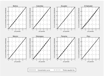
First, to study access to primary and secondary schools we focus on net enrolment rates. Tables 5.1 and 5.2 present the distributions of students (panel a) and net enrolment rates (panel b) by quintiles for each educational level. Corresponding concentration curves are shown in Figures 5.1 and 5.2.
Enrolment rates at the primary school level are very high in LA, ranging from 89.6% in El Salvador to 98% in Mexico. Though increasing with per capita consumption, enrolment rates are high even in the poorest quintile (between 78% and 96%). For the upper quintiles, enrolment rates are almost perfect. Figure 5.1 shows the corresponding concentration curves, which almost overlap with the perfect equality line.
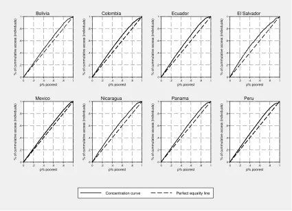
As expected, enrolment rates are lower at the secondary school level, ranging from 33.3% in El Salvador to 76.4% in Peru. Also, differences in enrolment rates between the poorest and the richest quintile are considerable (between 35 and 72 percentage points). This is illustrated in Figure 5.2 by concentration curves to the right of the perfect equality line.
So far, the distribution of access to primary and secondary education do not exhibit concentration levels that seem enough to explain the observed pro-rich distribution of expenditures on education described in Section 4. Therefore, we next consider another dimension of access to education: access to high quality education. It is likely that children from the richest quintiles have more access to higher quality education. Quality gap among schools could be due to differences in teaching, class size, facilities, and budgets, among other factors. And all these characteristics usually differ between public and private schools.17
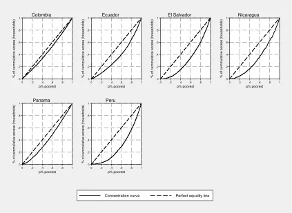
Tables 5.3 and 5.4 report the proportion of enrolled students attending public primary and secondary schools, respectively. In LA countries, most children study at public schools: from 73% to 92.1% (69.5% to 88.7%) of students enrolled at the primary (secondary) level, attend public schools. But while almost all children from the poorest quintile attend public schools, most children from the 20% richest households attend private schools. Indeed, the concentration curves located to the left of the perfect equality line in Figures 5.3 and 5.4 indicate a pro-poor concentration of the access to public education at the primary and secondary level.
Summing up, a pro-rich concentration of access to private primary and secondary schools, in addition to a pro-rich concentration of access to secondary education, help explain the observed pro-rich concentration of household expenditures on education. Of course, access to colleges and universities may well contribute to the explanation.
Access to Health Services
As for the case of education services, the pro-rich distribution characterizing health expenditures could be due to both, the fact that access is concentrated on the upper quintiles, and because the quality of health services that access poor and rich families is different.
17 There is a wide literature and evidence on this topic. See for instance Card and Krueger (1992) and Kingdon
We use two alternative indicators to measure access to health services: whether the household head is covered by a health insurance (Table and Figure 5.5), and whether any household member received any kind of professional medical care when needed (Table and Figure 5.6).
As Table 5.5 shows, access to health insurance appears to be very limited in some LA countries, such as Nicaragua (17.2%), and to a lesser extent El Salvador (28.6%), Peru (29.1%), and Ecuador (35.4%). Health insurance coverage is higher in Colombia (67.7%) and Panama (58.9%).
Health insurance coverage is strongly concentrated on the upper quintiles: depending on the country, between 3.7% and 53.8% of heads of households from the poorest quintile are insured, while corresponding figures for the richest quintile range from 32.6% to 83.9%.
When performing both intra and inter country comparisons, distribution of access to medical services is much more egalitarian than that of health insurance coverage. Depending on the country, concentration coefficients for the former go from 1.3 to 9.6, while they range from 9.3 to 41.9 for the latter. Also, as can be seen in Figures 5.5 and 5.6, concentration curves corresponding to health insurance coverage are further from the perfect equality line than those corresponding to access to medical services.
As for the case of education, taking into account differences in the quality of health services accessed by poorer and richer households, would help to understand the observed expenditure patterns. Unfortunately, most surveys lack this kind of information.
Access to Fixed and Mobile Telephones
Access to fixed phones is rather limited in LA countries. As shown in Table 5.7, the percentage of households with access to a fixed phone ranges from 14.2% in Nicaragua to a maximum of 54.6% in Colombia. Moreover, the distribution of telephone access is extremely concentrated on the upper quintiles. For example, only 1% of households from the poorest quintile in Peru have a fixed phone compared to almost 70% of households from the richest quintile. Thus, the corresponding concentration curves are located far to the right of the perfect equality line, as can be seen in Figure 5.7.
This high pro-rich concentration of the distribution of access explains much of the also high pro-rich concentration of the expenditures on fixed phones discussed in Section 4.
The distribution of access to mobile phones is described in Table and Figure 5.8. Access to cell phones varies between 17.5% in Colombia to 68.2% in Ecuador. Considering median values of coverage across countries, approximately 36% of households have fixed and cell phones. As mentioned above, Colombia has the highest fixed phone access (54.6%), but it also has the lowest cell phone coverage (17.5%). Although this suggests some kind of substitution in the consumption of the two services, the case of Colombia seems to be the exception rather than the rule: for the rest of the countries wider fixed phone coverage is associated to wider cell phone coverage (Spearman´s rank correlation equals 64%).
Even though access to cell phones is also concentrated on the upper quintiles, the use of mobile phones is more common among poor households than the access to fixed telephones.
Access to a Home Internet Connection
Access to internet at home is very rare in LA, reaching a maximum coverage of 8.4% in Mexico, followed by Colombia (5.3%), Panama (5.0%), and Peru (4.7%). As expected, internet access is extremely pro-rich concentrated, and there are virtually no households from the poorer quintiles with home internet connection.
Access to Transport Services (Public and Private)
As was mentioned earlier, for most countries there is no available information on the use of transport services. Therefore, access will be proxied by an indicator of positive household expenditure on transport services, both private and public. Under this definition, no access to transport services means that the family does not report positive expenditures on any means of transport, presumably because it does not use any.
As Table 5.10 shows, depending on the country, between 65.2% and 90.9% of households use either public or private transport services. The distribution of access exhibit a slight pro-rich concentration (see Figure 5.10), but still access vary markedly by quintiles. For example, in Peru, Colombia and Ecuador, half or more of the families from the poorest quintile do not pay for the use of transport services (because probably they do not use any), while more than 80% of the families from the richest quintile do.
Access to Water
We use two alternative indicators of access to water services. According to the first indicator, a household have access to water if it has a source of (presumably) drinkable water in its terrain or dwelling. According to the second one, a household has access to water if it is connected to a water network. Clearly, if a household have access to water based on the latter definition, then it also has access to water based on the former. Tables 5.11 and 5.12 describe the distribution of access to water across consumption quintiles based on both indicators, and Figures 5.11 and 5.12 illustrate the corresponding concentration curves.
Depending on the country, between 71.1% and 96.1% of the households have access to any source of drinkable water in their terrains or dwellings, while the proportion ranges from 64.6% to 90.3% when we focus on households connected to a water network. In both cases, the distribution of access is slightly pro-rich, with low to moderate concentration indices. In spite of this, access to a source of drinkable water is very limited for poor households in some countries. In Peru, for example, almost 60% of households from the first quintile, and 40% from the second one, do not have access to drinkable water in their terrains or dwellings.
From this analysis we conclude that the somewhat low concentration of access to water do not seem enough to account for the observed moderate pro-rich distribution of household expenditures on water. Hence, the latter must be explained by variations in prices faced and amounts consumed by households from different segments of the consumption distribution
Access to Electricity
Coverage of electricity networks is almost perfect in some of the countries under analysis. This is the case in Mexico, Ecuador, and to a lesser extent, in Colombia, where 98.4%, 97.4%, and 95.7% of households have electricity, respectively. Furthermore, coverage is very high even among poor households: at least 90% of households from the first quintile have access to electricity services in those countries (see Table and Figure 5.13).
Access to Gas
As for the other basic services, it would be interesting to study the distribution of access to natural gas networks, but in most of the countries under analysis households only access to bottled gas (liquefied petroleum gas or LPG). There are no natural gas networks in Ecuador, El Salvador, Nicaragua, Panama, and Peru. On the other hand, in countries like Bolivia and Brazil, even though natural gas networks are available, the residential coverage is very low (below 2% of households) because of climatic reasons.18
6. Main findings and final remarks
The aim of this paper was to describe the way services are used by the population, especially the poorest segments. To this end, a distributional incidence analysis was performed to study the patterns describing access to and expenditures on basic services in eight Latin American countries: Bolivia, Colombia, Ecuador, El Salvador, Mexico, Nicaragua, Panama and Peru. The services considered were the social services education and health; the infrastructure services public transport, water, electricity, and gas; and the telecommunication services fixed and mobile telephone.
We found that all these services present pro-rich distributions, i.e. household expenditures increase as household per capita consumption goes up. The highest concentration indices are found for the distributions of expenditures on telecommunication services, causing expenditure shares to markedly increase with household consumption and Kakwani indices to take positive high values. Social services present a moderate concentration, and, consequently, shares increase moderately as we move from the poorer to the richer quintiles. Concerning infrastructure services (except gas), expenditures are characterized by the lowest pro-rich concentration, so in most cases shares diminish as household consumption rises. Furthermore, from the distributional analysis of access we found that the poorest households usually face limited access to services (or to quality services), and this fact explains much of the observed expenditure patterns.
These findings suggest that the distributional effects of potential reforms of services sectors should be small. Intuitively, if services with a high participation on total household consumption also present sharp share-consumption patterns (positive or negative), the distributional effect would be strong. However, in our case the services with the highest shares (education, health, and transport) are characterized by moderate to small Kakwani indices, while services with high Kakwani indices (telecommunication and gas) represent a small part of total household consumption. In fact, based on some simple micro-simulation exercises, we found that inequality changes are very small, even when the prices of all services under analysis rise by a 30%19.
18 A distributional incidence analysis of the access to gas networks for the Argentinean case can be found in
Marchionni, et al. (2008).
19 For other developing countries, other studies find that reforms (price changes) might have distributive effects. See
Appendix A. Definitions of expenditure items.
This appendix briefly describes the main items that constitute the total household expenditure on each service.
Expenditures on education. It includes monthly expenditures of all family members on
items such as school fees, tuition, uniforms, textbooks, and school transportation. Other items appear explicitly in some countries’ surveys. This is the case of contributions to parents’ associations (Bolivia, Ecuador, Nicaragua and Peru), and expenditures on meals at school (Colombia and Nicaragua). But it is not possible to know whether these items are included within the item labeled “other expenditures on education” in the other countries’ questionnaires. Finally, El Salvador was excluded from the analysis of expenditures on education because some key expenditure items were missing from the corresponding database (actually, a whole expenditure section is missing from it).
Expenditures on Health. It includes monthly expenditures of all family members on items
such as medicines, professional medical care, clinical analysis and other routine studies. Again, some items are explicitly mentioned in some questionnaires but no in others. For instance, hospitalization expenditures are explicitly considered in all countries except Colombia and Panama; health insurance costs appear in all countries but Peru and Bolivia; and surveys in Ecuador, Mexico, Nicaragua and Peru include questions on health expenditures related to pregnancy and childbirth. Finally, all countries except Bolivia and Colombia include the item labeled “other health expenditures”, which is not explicitly defined and that may contain any item not explicitly mentioned in the questionnaires.
Again, El Salvador was also removed from the analysis of health expenditures because some key expenditure items were missing from the database.
Expenditures on fixed and mobile telephone, and total telecommunication services.
Telephone expenditures comprise monthly household expenditures on both fixed and cell phones. In the latter case, it includes expenditures by all family members. For all countries but Nicaragua, disaggregated information for the two services is available.
Concerning total telecommunication expenditures, monthly expenditures on other items such as public telephones, postal services and internet connection are included, beside fixed and mobile phone. For El Salvador there is no information on other telecommunication services so that total telecommunication expenditure only includes fixed and cellular phone.
Expenditures on public transportation. It includes monthly expenditures of all family
members on any public transportation means (urban, interurban and international). As particular cases, there are no information on international trips and airplane tickets for Bolivia, and public telephone expenditures are reported joint with transport expenditures in Peru. As for the case of education and health expenditures, El Salvador is excluded from the analysis of public transportation expenditures. Panama is also removed from this analysis since only 15% of households in the sample have information on public transportation expenditures.
Expenditure on water. It includes monthly expenditures on water for household
consumption. In the cases of El Salvador and Panama, when the rent paid by a household include water expenditure, National Statistical Offices estimate households’ expenditures on water based on information from other households.
Expenditure on electricity. It includes monthly expenditures on electricity for household
consumption. As for water expenditures, in El Salvador and Panama, National Statistical Offices estimate household electricity expenditures when this item is included in the rent paid by the household.
Expenditure on Gas. It includes monthly expenditures on gas for household consumption
households only access to liquefied petroleum gas (LPG). There are no natural gas networks in Ecuador, El Salvador, Nicaragua, Panama, and Peru, and even when there are, like in Bolivia and Brazil, the residential coverage is very low (below 2% of households) because of climatic reasons.
Appendix B. Access to services along the income distribution.
All Latin American countries.
For the analyses of expenditures and access performed in Sections 4 and 5 only eight LA countries are considered: Bolivia, Colombia, Ecuador, El Salvador, Mexico, Nicaragua, Panama, and Peru. These are the only LA countries for which we have information on household expenditures on services and household total consumption (or expenditure, depending on the country). Even when data on access to services is available in almost all household surveys, for the other LA countries we lack information on household total consumption, which is the variable we use to proxy household well-being.
References
Amemiya, T. (1985). Advanced Econometrics. Hardvard University Press.
Bourguignon, F and Pereira da Silva (eds.) (2003). The impact of economic policies on poverty and income distribution. The World Bank and Oxford University Press.
Card, D. and A. B. Krueger (1992). “Does school quality matter? Returns to Education and the Characteristics of Public Schools in the United States.” Journal of Political Economy,
University of Chicago Press, vol. 100(1), pp. 1-40, February.
CEDLAS (2007). A Guide to SEDLAC. www.depeco.econo.unlp.edu.ar/cedlas/sedlac. Cont, W., Hancevic, P. And Navajas, F. (2009). “Energy populism and household welfare”,
AAEP, November 2009.
Deaton, A. and S. Zaidi (2002). “Guidelines for Constructing Consumption Aggregates for Welfare Analysis.” Living Standards Measurement Study Working Paper: 135. v. 104, pp. xi, Washington, D.C.: The World Bank
Kingdon, G. (1996). “The quality and efficiency of private and public education: a case study of rural India.”Oxford Bulletin of Economics and Statistics, Department of Economics,
University of Oxford, vol. 58(1), pp. 57-82, February.
Komives, K., V. Foster, J. Halpern, and Q. Wodon (2005). Water, Electricity and the Poor. Who Benefits from Utility Subsidies?. The World Bank.
Lambert, P. (2001). The distribution and redistribution of income. Manchester University Press.
Marchionni, M., W. Sosa Escudero and J. Alejo (2008). “La incidencia distributiva del acceso, gasto y consumo de los Servicios Públicos.” In Navajas F. (editor), La Tarifa Social en los Sectores de Infraestructura en la Argentina, Buenos Aires: TEMAS.
Van de Walle, D. (2003). “Behavioral incidence analysis of public spending and social programs.” In Bourguignon and Pereira da Silva (eds.), The impact of economic policies on poverty and income distribution. The World Bank and Oxford University
Tables and figures
Table 3.1. Countries and surveys included in the analysis
expenditure on services
Argentina Encuesta Permanente de Hogares-Continua 2006 x
Bolivia Encuesta Continua de Hogares- MECOVI 2005 x x x
Brazil Pesquisa Nacional por Amostra de Domicilios 2006 x
Chile Encuesta de Caracterización Socioeconómica Nacional 2006 x
Colombia Encuesta de Calidad de Vida 2003 x x x
Costa Rica Encuesta de Hogares de Propósitos Múltiples 2005 x
Dominican Rep. Encuesta Nacional de Fuerza de Trabajo 2006 x
Ecuador Encuesta de Condiciones de Vida 2006 x x x
El Salvador Encuesta de Hogares de Propósitos Múltiples 2005 x x x
Guatemala Encuesta Condiciones de Vida 2006 x
Honduras Encuesta Permanente de Hogares de Propósitos Múltiples 2006 x
Mexico Encuesta Nacional de Ingresos y Gastos de los Hogares 2006 x x x
Nicaragua Encuesta Nacional de Hogares sobre Medición de Nivel de Vida 2005 x x x
Panama Encuesta de Calidad de Vida 2003 x x x
Paraguay Encuesta Permanente de Hogares 2005 x
Peru Encuesta Nacional de Hogares 2006 x x x
Uruguay Encuesta Continua de Hogares 2006 x
Venezuela Encuesta de Hogares Por Muestreo 2005 x
Variable used to proxy household well-being household per
capita income*
Source: authors' own calculations based on SEDLAC (CEDLAS and The World Bank) * Results are presented in Appendix B
household per capita consumption or expenditure
Country Survey name and year
access to services Countries included in the analysis of
Table 4.1. Expenditure on services as a percentage of total household consumption
Fixed phone Cell phone Total Public Transport Water Electricity Gas
Bolivia** 6.5% 1.8% 0.5% 1.0% 1.8% 3.9% 1.2% 2.8% 1.4% 19.4% Colombia** 4.0% 5.5% 3.8% 1.0% 5.0% 10.4% 2.4% 5.0% 2.7% 34.8% Ecuador 6.6% 8.0% 1.0% 1.9% 3.8% 8.6% 1.3% 2.6% 0.7% 31.5% El Salvador** 8.2% 1.2% 2.2% 1.1% 3.3% 3.7% 2.3% 4.4% 0.9% 24.0% Mexico 5.3% 2.6% 1.6% 1.1% 3.1% 5.0% 0.7% 2.3% 1.9% 20.9% Nicaragua 4.8% 7.3% NA NA 1.5% 4.3% 1.2% 2.0% 1.1% 22.1% Panama 5.3% 5.6% 1.3% 0.9% 2.3% 0.8% 1.0% 2.6% 0.7% 18.2% Peru 4.2% 3.4% 0.8% 0.4% 1.4% 5.3% 1.0% 1.7% 1.1% 18.1%
Source: authors' own calculations based on SEDLAC (CEDLAS and The World Bank) Note: ** Expenditure on services as a share of household total expenditure.
Infrastructure Services
Country Education Health Telecommunication Total
S ource: authors' own calculations based on SEDLAC (CEDLAS and The Worl d Bank) 0%
10% 20% 30% 40% 50% 60% 70% 80% 90% 100%
B
o
liv
ia
C
o
lo
m
b
ia
E
c
u
a
d
o
r
E
l S
a
lv
a
d
o
r
M
e
x
ic
o
N
ic
a
ra
g
u
a
P
a
n
a
m
a
P
e
ru
Table 4.2. Expenditures on education by consumption quintiles
(a) Distribution of expenditures on Education
1 2 3 4 5
Bolivia** 3.5% 6.6% 13.0% 19.1% 57.8% 100% 52.2
Colombia** 6.6% 9.9% 15.6% 24.0% 43.9% 100% 37.6
Ecuador 6.2% 9.1% 13.6% 22.9% 48.2% 100% 41.4
El Salvador** NA NA NA NA NA NA NA
Mexico 5.8% 9.8% 14.2% 19.1% 51.1% 100% 43.2
Nicaragua 5.2% 10.0% 17.2% 23.3% 44.4% 100% 39.6
Panama 6.9% 12.9% 17.4% 23.2% 39.5% 100% 32.3
Peru 3.5% 6.3% 12.0% 21.0% 57.2% 100% 52.4
(b) Expenditures on Education as a share of household total consumption
1 2 3 4 5
Bolivia** 4.5% 4.6% 6.1% 6.5% 10.8% 6.5% 17.8
Colombia** 4.5% 3.5% 4.1% 4.3% 3.7% 4.0% -1,2×
Ecuador 5.7% 5.7% 6.5% 7.4% 7.7% 6.6% 7.7
El Salvador** NA NA NA NA NA NA NA
Mexico 4.8% 5.1% 5.4% 5.2% 6.1% 5.3% 7.5
Nicaragua 3.0% 3.9% 5.3% 5.6% 6.0% 4.8% 11.4
Panama 4.6% 5.9% 5.8% 5.4% 4.9% 5.3% 0,2×
Peru 2.6% 2.8% 3.8% 4.9% 6.9% 4.2% 19.3
Source: authors' own calculations based on SEDLAC (CEDLAS and The World Bank) Note: ** Expenditure on services as a share of household total expenditure.
All concentration and Kakwani indices are significant at a 10% level (by bootstrap), except when indicated by ×.
Concentration index
Kakwani index Total
Country quintiles of per capita household consumption Total
Country quintiles of per capita household consumption
Figure 4.2. Concentration curves for expenditures on education.
0 .2 .4 .6 .8 1 % o f c u m m u la ti v e e x p e n d it u re
0 .2 .4 .6 .8 1
p% poorest Bolivia 0 .2 .4 .6 .8 1 % o f c u m m u la ti v e e x p e n d it u re
0 .2 .4 .6 .8 1
p% poorest Colombia 0 .2 .4 .6 .8 1 % o f c u m m u la ti v e e x p e n d it u re
0 .2 .4 .6 .8 1
p% poorest Ecuador 0 .2 .4 .6 .8 1 % o f c u m m u la ti v e e x p e n d it u re
0 .2 .4 .6 .8 1
p% poorest Mexico 0 .2 .4 .6 .8 1 % o f c u m m u la ti v e e x p e n d it u re
0 .2 .4 .6 .8 1
p% poorest Nicaragua 0 .2 .4 .6 .8 1 % o f c u m m u la ti v e e x p e n d it u re
0 .2 .4 .6 .8 1
p% poorest Panama 0 .2 .4 .6 .8 1 % o f c u m m u la ti v e e x p e n d it u re
0 .2 .4 .6 .8 1
p% poorest
Peru
Concentration curve Lorenz curve Perfect equality line
Table 4.3. Expenditures on health by consumption quintiles
(a) Distribution of expenditure on Health
1 2 3 4 5
Bolivia** 2.4% 7.1% 14.1% 21.2% 55.1% 100% 51.4
Colombia** 2.8% 7.9% 12.5% 20.9% 55.9% 100% 51.6
Ecuador 8.7% 12.4% 14.6% 21.0% 43.4% 100% 33.5
El Salvador** NA NA NA NA NA NA NA
Mexico 5.4% 9.6% 13.9% 21.4% 49.8% 100% 44.3
Nicaragua 5.8% 10.1% 17.3% 20.1% 46.8% 100% 40.2
Panama 8.5% 11.3% 13.6% 17.9% 48.7% 100% 38.2
Peru 4.0% 8.7% 15.8% 23.6% 48.0% 100% 43.7
(b) Expenditure on Health as a share of household total consumption
1 2 3 4 5
Bolivia** 0.9% 1.3% 1.9% 2.0% 2.8% 1.8% 17.0
Colombia** 2.9% 4.5% 5.5% 6.6% 8.0% 5.5% 12.8
Ecuador 8.5% 8.5% 7.2% 7.7% 8.0% 8.0% -0,2×
El Salvador** NA NA NA NA NA NA NA
Mexico 2.0% 2.4% 2.6% 2.9% 3.0% 2.6% 8.6
Nicaragua 4.8% 5.9% 7.8% 7.1% 10.9% 7.3% 12.0
Panama 7.1% 5.2% 5.0% 4.7% 6.3% 5.6% 6.1
Peru 1.9% 2.8% 3.6% 4.1% 4.7% 3.4% 10.6
Source: authors' own calculations based on SEDLAC (CEDLAS and The World Bank) Note: ** Expenditure on services as a share of household total expenditure.
All concentration and Kakwani indices are significant at a 10% level (by bootstrap), except when indicated by ×.
Concentration index
Kakwani index Total
Country quintiles of per capita household consumption Total
Country quintiles of per capita household consumption
Figure 4.3. Concentration curves for expenditures on health.
0 .2 .4 .6 .8 1 % o f c u m m u la ti v e e x p e n d it u re
0 .2 .4 .6 .8 1
p% poorest Bolivia 0 .2 .4 .6 .8 1 % o f c u m m u la ti v e e x p e n d it u re
0 .2 .4 .6 .8 1
p% poorest Colombia 0 .2 .4 .6 .8 1 % o f c u m m u la ti v e e x p e n d it u re
0 .2 .4 .6 .8 1
p% poorest Ecuador 0 .2 .4 .6 .8 1 % o f c u m m u la ti v e e x p e n d it u re
0 .2 .4 .6 .8 1
p% poorest Mexico 0 .2 .4 .6 .8 1 % o f c u m m u la ti v e e x p e n d it u re
0 .2 .4 .6 .8 1
p% poorest Nicaragua 0 .2 .4 .6 .8 1 % o f c u m m u la ti v e e x p e n d it u re
0 .2 .4 .6 .8 1
p% poorest Panama 0 .2 .4 .6 .8 1 % o f c u m m u la ti v e e x p e n d it u re
0 .2 .4 .6 .8 1
p% poorest
Peru
Concentration curve Lorenz curve Perfect equality line
Table 4.4. Expenditures on fixed telephone by consumption quintiles
(a) Distribution of expenditure on Fixed Telephone
1 2 3 4 5
Bolivia** 0.1% 1.3% 5.0% 17.9% 75.7% 100% 71.4
Colombia** 3.9% 9.0% 15.0% 23.8% 48.2% 100% 44.4
Ecuador 1.6% 5.5% 12.9% 26.0% 53.9% 100% 52.8
El Salvador** 2.0% 8.3% 16.0% 25.5% 48.1% 100% 46.3
Mexico 3.8% 10.9% 18.3% 27.0% 40.0% 100% 37.6
Nicaragua NA NA NA NA NA NA NA
Panama 1.0% 6.1% 12.5% 23.5% 57.0% 100% 55.5
Peru 0.5% 3.6% 10.3% 24.7% 60.8% 100% 60.5
(b) Expenditure on Fixed Telephone as a share of household total consumption
1 2 3 4 5
Bolivia** 0.0% 0.1% 0.3% 0.7% 1.4% 0.5% 37.0
Colombia** 2.5% 3.0% 4.0% 4.5% 4.7% 3.8% 5.5
Ecuador 0.2% 0.6% 1.1% 1.6% 1.8% 1.0% 19.1
El Salvador** 0.6% 1.7% 2.5% 2.9% 3.2% 2.2% 14.2
Mexico 0.7% 1.5% 2.0% 2.2% 1.8% 1.6% 1.8
Nicaragua NA NA NA NA NA NA NA
Panama 0.2% 0.7% 1.2% 1.7% 2.4% 1.3% 23.6
Peru 0.1% 0.3% 0.6% 1.2% 1.8% 0.8% 27.4
Source: authors' own calculations based on SEDLAC (CEDLAS and The World Bank) Note: ** Expenditure on services as a share of household total expenditure.
All concentration and Kakwani indices are significant at a 10% level (by bootstrap), except when indicated by ×.
Concentration index
Kakwani index Total
Country quintiles of per capita household consumption Total
Country quintiles of per capita household consumption
Figure 4.4. Concentration curves for expenditures on fixed telephone
0 .2 .4 .6 .8 1 % o f c u m m u la ti v e e x p e n d it u re
0 .2 .4 .6 .8 1
p% poorest Bolivia 0 .2 .4 .6 .8 1 % o f c u m m u la ti v e e x p e n d it u re
0 .2 .4 .6 .8 1
p% poorest Colombia 0 .2 .4 .6 .8 1 % o f c u m m u la ti v e e x p e n d it u re
0 .2 .4 .6 .8 1
p% poorest Ecuador 0 .2 .4 .6 .8 1 % o f c u m m u la ti v e e x p e n d it u re
0 .2 .4 .6 .8 1
p% poorest El Salvador 0 .2 .4 .6 .8 1 % o f c u m m u la ti v e e x p e n d it u re
0 .2 .4 .6 .8 1
p% poorest Mexico 0 .2 .4 .6 .8 1 % o f c u m m u la ti v e e x p e n d it u re
0 .2 .4 .6 .8 1
p% poorest Panama 0 .2 .4 .6 .8 1 % o f c u m m u la ti v e e x p e n d it u re
0 .2 .4 .6 .8 1
p% poorest
Peru
Concentration curve Lorenz curve Perfect equality line
Table 4.5. Expenditures on cell telephone by consumption quintiles
(a) Distribution of expenditure on Mobile Telephone
1 2 3 4 5
Bolivia** 1.4% 6.1% 13.3% 21.8% 57.4% 100% 55.7
Colombia** 1.1% 4.1% 8.7% 17.7% 68.4% 100% 64.3
Ecuador 5.5% 9.8% 14.2% 23.3% 47.2% 100% 41.2
El Salvador** 3.0% 7.1% 10.5% 18.3% 61.2% 100% 55.2
Mexico 4.1% 8.6% 15.3% 22.8% 49.2% 100% 44.3
Nicaragua NA NA NA NA NA NA NA
Panama 2.3% 6.9% 12.6% 21.7% 56.5% 100% 54.4
Peru 0.8% 4.2% 10.1% 21.2% 63.8% 100% 62.2
(b) Expenditure on Mobile Telephone as a share of household total consumption
1 2 3 4 5
Bolivia** 0.2% 0.6% 1.0% 1.3% 1.7% 1.0% 21.3
Colombia** 0.4% 0.5% 0.8% 1.2% 2.2% 1.0% 25.5
Ecuador 1.3% 1.7% 1.9% 2.2% 2.2% 1.9% 7.5
El Salvador** 0.5% 0.8% 0.9% 1.1% 2.0% 1.1% 23.1
Mexico 0.6% 0.9% 1.1% 1.3% 1.5% 1.1% 8.6
Nicaragua NA NA NA NA NA NA NA
Panama 0.3% 0.7% 0.9% 1.1% 1.6% 0.9% 22.6
Peru 0.1% 0.2% 0.3% 0.5% 0.9% 0.4% 29.2
Source: authors' own calculations based on SEDLAC (CEDLAS and The World Bank) Note: ** Expenditure on services as a share of household total expenditure.
All concentration and Kakwani indices are significant at a 10% level (by bootstrap), except when indicated by ×.
Concentration index
Kakwani index Total
Country quintiles of per capita household consumption Total
Country quintiles of per capita household consumption
Figure 4.5. Concentration curves for expenditures on cell telephone
0 .2 .4 .6 .8 1 % o f c u m m u la ti v e e x p e n d it u re
0 .2 .4 .6 .8 1
p% poorest Bolivia 0 .2 .4 .6 .8 1 % o f c u m m u la ti v e e x p e n d it u re
0 .2 .4 .6 .8 1
p% poorest Colombia 0 .2 .4 .6 .8 1 % o f c u m m u la ti v e e x p e n d it u re
0 .2 .4 .6 .8 1
p% poorest Ecuador 0 .2 .4 .6 .8 1 % o f c u m m u la ti v e e x p e n d it u re
0 .2 .4 .6 .8 1
p% poorest El Salvador 0 .2 .4 .6 .8 1 % o f c u m m u la ti v e e x p e n d it u re
0 .2 .4 .6 .8 1
p% poorest Mexico 0 .2 .4 .6 .8 1 % o f c u m m u la ti v e e x p e n d it u re
0 .2 .4 .6 .8 1
p% poorest Panama 0 .2 .4 .6 .8 1 % o f c u m m u la ti v e e x p e n d it u re
0 .2 .4 .6 .8 1
p% poorest
Peru
Concentration curve Lorenz curve Perfect equality line