Finite Deformation of Porous Elastomers: A Computational Micromechanics Approach

Finite deformation of porous elastomers: a computational

micromechanics approach

J. MORALEDA , J. SEGURADO and J. LLORCA Departamento de Ciencia de Materiales, Universidad Politécnica de Madrid Instituto Madrileño de Estudios Avanzados en Materiales (IMDEA-materiales),

E. T. S. de Ingenieros de Caminos, 28040 -Madrid, Spain

The finite deformation of porous elastomers was studied by means of the numerical simulation of a representative volume element of the microstructure. The size and the discretization of the volume element were selected to obtain an exact response (to a f e w percent) of the plane-strain deformation of a material made up of a random and isotropic dispersión of circular cylindrical voids embedded in an incompressible neo-Hookean matrix. Three different loading modes (in-plane isotropic deformation, uniaxial elongation, and uniaxial traction) were simulated, and the corresponding stress—strain curves as well as the evolution of the microstructure with deformation were presented for materials with an initial porosity of 5, 10 and 20%. The numerical results were compared with the available homogenization models for the finite deformation of porous elastomers. It was found that the second-order estímate with field fluctuations of López-Pamiés and Ponte Castañeda led to very good approximations to the numerical results in most cases, and significant differences were only found under conditions of highly constrained deformation. The sources of these differences were discussed in the light of the changes in the microstructure provided by the numerical simulations.

1. Introduction

Applications oí this methodology to take into account the nonlinear material behaviour require a linearization procedure to re-write the local constitutive laws in such a way that homogenization schemes valid in linear thermoelasticity might apply, and they have been developed in the context oí tangent, secant and affine approximations . Although there has been considerable progress in this área in recent years, it should be noted that the nonlinear versions oí the homogenization models are rather more complex and do not always capture accurately the effective behaviour oí the composite. Further extensions to take into account elastomeric phases were hindered by the diffículties associated with the strong nonlinear behaviour oí elastomers and with the evolution oí the microstructure (size, shape, position and orientation oí the inclusions) as a result oí the fínite changes in geometry upon loading. Although a proper homogenization framework to study elastomeric-matrix composites with random microstructures was developed at the beginning oí the 1970s , most oí the work was restricted to composites with periodic microstructures or to particular loading cases , and more general models have appeared very recently

Within the context oí porous elastomers, the fírst constitutive model is credited to Blatz and Ko , who proposed a phenomenological expression for the strain energy function from experiments carried out in voided polyurethane rubber. Abeyaratne and Triantafyllidis carried out a numerical study oí the behaviour oí a nearly incompressible neo-Hookean matrix with periodic cylindrical pores and determined the behaviour oí the composite from these results using the homogenization theory. Danielsson estimated the strain energy function of the porous material from the kinematically admissible deformation fíelds in a simple micromechanical model of a spherical matrix with a spherical hole which transforms into an ellipsoid under the action of three principal stretches. The fírst application of a homogenization model for a porous elastomer containing a random dispersión of spherical voids is found in the work of Hashin , who obtained an exact solution for the particular case of isotropic elastic deformation. Explicit results for the general deformation of a random distribution of aligned cylindrical pores embedded in an isotropic and incompressible elastomeric matrix

Computational micromechanics is another strategy to determine the behaviour of heterogeneous materials from the numerical simulation of the mechanical response of a represent volume element (RVE) of the microstructure whose size is large enough so that the effective properties computed from the RVE are independent of its size and position within the material. This new methodology has been successfully applied to analyze the mechanical response of sphere-reinforced composites in the elastic , elasto-plastic , visco-plastic regime

as well as in the presence of damage , and it is applied in the paper to analyze the deformation of a porous elastomer made up of a random and isotropic dispersión of cylindrical pores in an incompressible neo-Hookean matrix subjected to three different loading cases: isotropic tensile deformation, uniaxial tensile deformation and uniaxial traction. The simulations provide exact results (to a few percent) of the porous elastomer behaviour, which can be used as benchmarks to assess the accuracy of the homogenization models for porous elastomers

loading, which can be integrated over the corresponding volumes to obtain the average valúes of the field quantities. This information is used to understand the limitations of the current homogenization schemes and to point out the critical issues which should be addressed to improve the accuracy of the predictions.

2. Homogenization methods for elastomeric composites

Homogenization methods try to determine the effective composite behaviour in terms of the behaviour of each phase and of their spatial distribution. As indicated in the introduction, this is a challenging problem if one or more phases in the composite present an elastomeric behaviour due to the strong nonlinear behaviour of elastomers and to the evolution of the microstructure as a result of the finite deformations. The homogenization strategy in these materials consists of finding the effective strain energy of the composite, W, as a function of the average of the deformation gradient over the composite microstructure, F, . As a general case, let us consider a material made up of TV different phases distributed over a volume £20

in the reference configuration. The behaviour of each phase r is defined by its strain energy function W^(F), where F is the deformation gradient tensor. The local strain energy function in the composite can then be defined as

N

fT(X,F) = ^X« ( X ) ^ ( F ) (1)

r=\

in which X stands for the position vector of a point in the reference configuration and the functions yiA describe the microstructure of the composite according to:

M í 1, if X e d?

X(r)(X)= ' f M (2)

0, i X<jt£2

The effective strain energy function of the composite subjected to an average deformation gradient F can then be defined as

N

W(F) = min (W(X,F)) = min V c ^ ^ r f (3)

where cA = (xA) stands for the volume fraction of the phase r in the reference

configuration. In the above expressions, the symbols (•) and (•) denote volume averages over the composite (S20) a nd over the phase r(QA). The set CK in which the

minimization problem is defined by

jír(F) = {F/3x = x(X) with F = Vxx in Q0, x = FX on d£20J (4)

and corresponds to the set of admissible deformation gradient tensor fields compatible with the applied overall deformation gradient F.

for W(F). The first one is to find a solution for equation (3) by making some reasonable assumptions on the spatial distribution, behaviour, and the valué of the strain gradient tensor in each phase. This approach is followed by the homogeniza-tion models of Hashin and López Pamiés and Ponte Castañeda , which are briefly outlined below. The second one, used by computational micromechanics, obtains a numerical solution for equation (3) over a finite volume, representative of the composite microstructure and it will be discussed in detail in section 3.

2.1 Hashin's modelfor isotropic deformation

Hashin [14] analyzed the behaviour of a porous, incompressible hyper-elastic matrix subjected to large, isotropic deformation. The model assumed that the material was formed by hollow spheres (or aligned cylinders in two dimensions) of different radius. The initial ratio between the internal and external sphere (cylinder) radii was constant and dictated by the initial void volume fraction. The spheres (cylinders) filled all the space, implying that there is a distribution in their radii ranging to the infinitesimally small, which corresponds to the particular microstructure known as the composite sphere (cylinder) assemblage model. In the particular case of a two-dimensional arrangement of hollow cylinders subjected to in-plane isotropic deformation under plane-strain conditions, the elasticity problem can be solved by assuming that the section of the hollow fibres will remain circular under isotropic deformation. The average deformation gradient F can be defined as

F„=X; F22=X; F33=l and Fy=0iii/j (5)

where X is the overall elongation in the in-plane directions (1 and 2). If the initial fibre radius is chosen as R = 1, the initial void radius is given by AJQ~, fo being the

initial void volume fraction in the porous elastomer. Assuming that the circular shape of the hollow fibre does not change during deformation, equation (3) can be computed over one of the fibres and reduced to

u r rlrTr V If1A ^ ,

rv(¥) = W(X, X) = - (XuA2)2]tRdR (6)

where 3>(A, i ,A,2) stands for the strain energy function of the matrix and X2 = X^

because of the incompressibility. The valué of Ai =f(R, X) can be obtained exactly by applying the incompressibility condition over a matrix ring,

leading to

^ i = A / l + — ^ — - (7)

If the matrix behaves as a neo-Hookean incompressible material, whose strain energy function under plañe strain (X3 = 1) is given by

in which \i stands for the elastomer shear modulus, the exact solution of equation (6) for the effective strain energy function of the porous elastomer, W, is given by

A

(I,X)=|(1

-1)

-

(9)

2.2 Second-order homogenization

While Hashin's model only provided results for a particular type of deformation and microstructure, more general results could be obtained by making use of a 'second-order' homogenization method, which can handle the strong nonlinear constraint of material incompressibility. This approximation was originally developed by Ponte-Castañeda within the framework of viscoplastic materials, and it was later extended by Lopez-Pamiés and Ponte-Castañeda to hyper-elastic solids and applied to porous elastomers . The key concept behind the second-order homogenization method for hyperelastic composites is the introduction of a 'fictitious' linear comparison composite (LCC), which is used to convert available linear homogenization estimates into new estimates for the nonlinear hyper-elastic material. The LCC presents the same microstructure as the nonlinear one (i.e. same Xr)) and the corresponding local strain energy function of the LCC, Wj, can be

expressed as

N

frr(X,F) = ^ X « ( X ) ^ ( F ) (10)

r=\

where stands for the strain energy function of each phase in the LCC, which is given by second-order Taylor approximation of the nonlinear strain energy functions for the nonlinear composite about certain uniform reference deformation gradient Fr,

^ ( F ) = ^ ( F ) + 9F() • (F - F) + - (F - F) • L^(F - F ) . (11)

In this expression, LQ is a fourth-order constant tensor which stands for stiffness tensor of phase r in the LCC. The valúes of Fr and LQ depend on the particular versión of the second-order estímate chosen (tangent, generalized secant,...), as shown below.

The strain energy function of phase r is then approximated as

^r)(F) w W$(F) + F<r)(Fw,L0 ). (12)

where F ^ ( F ^ , L Q ) is a corrector function defíned in [16], which measures the error introduced when W-y(F) is used instead of W^(F). The effective strain energy function of the nonlinear composite. W, is then expressed as

N

where

Wj{F, Fw, 4r )) = min JA c ^ j W$ (F)V" (14)

is the effective strain energy function of the LCC. Equation (13) is valid for any reference deformation gradients FQ and moduli, LQ and it is necessary to determine the values of these variables which minimize W. The different solutions to this optimization problem lead to different estimates of the second-order method [16]. Among them, the simplified version of the generalized secant estimate with fluctuations has been shown to render the exact solution for the evolution of the porosity for general finite deformations, and consequently the solution for the isotropic deformation of a porous elastomer with an isotropic and incompressible matrix is exact up to the third order of the infinitesimal strain . This estimate

assumes that the reference deformation gradient is given by

FW = F (15)

and computes LQ by optimizing the overall energy expression given by equation (13) with respect to them.

This version of the second-order estimate with fluctuations was particularized in [21] for the case of plane-strain deformation (X3 = 1) of a porous elastomer made up

of a neo-Hookean incompressible matrix containing a random and isotropic dispersion circular cylindrical voids. The effective modulus tensor of the matrix phase in the LCC was computed following the Hashin-Shtrikman estimate [28], which is appropriate for this type of microstructure. Moreover, WA2) = 0, the initial volume fraction of voids c(2) =f0 in the voided composite, and the average stress

tensor in the matrix (phase 1) is given by S = (1/(1 —fo))S as the stresses in the second phase are 0.

Under such conditions, the effective strain energy function of the porous material subjected to arbitrary elongations X\ and X2 is given by [21]

/7 PAV4 +P3V3 +P2V2 +P\V+nV

Wfr/2) =

2 (16)

where v is the solution of the quartic polynomial

I-4V4 + r3v3 + r2v2 + r\v + r0 = 0 (17)

and explicit expressions for the coefficients Po,pi,P2,P3,P4,qo,qi,q2,q3,q4,ri,r2,r3

and r4 (which depend only onf0, X\ andX2y) In addition, equation (16) reduces to

W{X,X) (1 +f0)X2 + /0 - 1 - 2Xy0(x2+f0-l) (18)

l - / o

3. Computational micromechanics approach

3.1 Generation of the representative volume element

In computational micromechanics, the solution of equation (3) for each loading case is obtained numerically by solving the corresponding boundary value problem over an RVE which represents the composite microstructure. The RVE selected for this particular problem is a square containing a random and isotropic dispersion of circular voids with the same radius, which stands for the transverse section of the porous elastomer. For the reasons stated below, it is assumed that the RVE is periodic and thus the microstructure of the material can be obtained by translating along the horizontal and vertical directions (figure 1).

The pore distribution in the RVE was generated using the Random Sequential Adsorption algorithm [29], which ensures a random, isotropic and homogeneous distribution of the pores within the RVE. In this strategy, the void

diameter, d, is determined from the initial volume fraction of voids, f0, and the

number of voids Nin the RVE. The coordinates of the void centres are generated

randomly and sequentially, and a new void is accepted if the distance between the centre of the void and the centre of the closest void generated previously is higher

than a minimum value (1.035d) chosen to ensure an adequate discretization of the

ligament between the voids. In addition, the void surface should not be too

close (0.05d) to the edges and corners of the RVE to prevent the presence of

distorted elements during meshing. This procedure is repeated until Nvoids have

Figure 2. Periodic square cell created from an RVE of the porous elastomer with/0 = 0.10 and i V=40. The inset to the right shows detail of the finite element discretization.

3.2 Finite element model

The numerical analysis of the RVE was carried out using the finite element model. To this end, the periodic RVE was transformed into a square cell by splitting the pores intersecting a cell face into the appropriate number of parts and copying them to the opposite faces, figure 2. The resulting area was meshed with quadratic triangles and the node positions on opposite faces were identical in order to apply periodic boundary conditions. Six-noded triangular hybrid elements (CPE6H in ABAQUS ) were used for the discretization. The hybrid version of the quadratic triangles - which incorporates the pressure as an independent degree of freedom - was used because of the matrix incompressibility. It should be noted that the discretization was extremely fine (figure 2) to accurately capture the gradients of the strain fields between the pores and to represent the distorted shape of the deformed cell after finite deformation.

Periodic boundary conditions were applied to the edges of the square cell because the continuity between neighbouring RVEs (which deform like jigsaw puzzles) is maintained and, in addition, because the effective behaviour derived under these conditions is always bounded by those obtained under imposed forces or displacements . Let x\ and x2 be the Cartesian coordinates corresponding

to axes parallel to the RVE edges and with origin at one corner of the RVE, and u(xi, %2) the displacement vector at a point with coordinates (x\, xj. The periodic boundary conditions can be expressed in terms of the displacement vectors Ui and u2, which stand for the relative displacement between opposite edges, according to

U(X\, 0) — U2 = u(x\, L)

u ( 0 , x2) - u i = u ( L , x2) (19)

deformation (X = X\ = X2) is applied with ui = ((X — \)L, 0) and 1 1 2 = (0, (X — 1)L), while uniaxial traction along the x\ axis is imposed with m = ((X — \)L, 0) and 1 1 2 = ((A,2 — V)L, 0) in which X2 is computed from the condition that the average forcé acting in the x2 direction over the edges x2 = 0 = L is zero.

The average nominal stress S normal to the edges oí the square cell is computed at any point oí the simulation as the total forcé divided by the initial edge length.

The matrix behaviour followed the neo-Hookean model in ABAQUS for an incompressible and isotropic hyperelastic solid. Simulations were carried out with Abaqus/Standard under plane-strain conditions and within the framework of the finite deformations theory with the initial unstressed state as reference.

3.3 Discretization and size of the R VE

The finite element discretization of the RVE has to be fine enough to accurately capture the gradients of the strain field between the pores and to represent the distorted shape of the deformed cell after finite deformation. There are not a priori estimates of the number of degrees of freedom necessary to obtain results independent of the discretization, and the influence of this factor was studied numerically. To this end, the same RVE containing 20 voids with f0 = 0.05 was

meshed with two levéis of refínement corresponding to 25 000 and 50 000 quadratic triangular elements. The stress-strain curves for isotropic in-plane deformation are plotted in figure 3. The curves are practically superposed in the whole deformation range, indicating that even the coarser mesh was able to resolve the strain gradients in the matrix. The only difference between both discretizations was the máximum strain that can be reached before the numerical simulation fails due to excessive distortion of one element. Obviously, fíner meshes led to larger strains and - as the computer time for the finer meshes was affordable - the degree of refínement corresponding to the mesh with 50000 elements was used in all the numerical simulations presented in the paper.

1 , 1 ,

0.2 0.4

elements

- - • - - 2 5 0 0 0

- ^ - 50000 i

0.6 0.8

-\n{X)

Figure 3. Results of the finite element simulation of an RVE containing 20 circular voids with/0 = 0.05 subjected to in-plane isotropic deformation (X = X\ = X2) with two different levéis of discretization (25 000 and 50000 quadratic triangular elements). The curves show the nominal stress (S = Sn = S22) vs. the logarithmic strain e = ln(A).

(a) 4 (b)4

Figure 4. Effect of the RVE size on the stress-strain curve under in-plane isotropic deformation. (a) RVE with a random and isotropic dispersión of 20 voids. (b) RVE with a random and isotropic dispersión of 40 voids. Each figure includes the stress-strain curves corresponding to three different void realizations.

the máximum difference in stresses among the RVEs with 20 voids was around 5%. Thus, an RVE with a random and isotropic dispersión of 40 voids was selected for the numerical simulations presented below. In order to improve the accuracy of the numerical predictions in the analyses with/0 = 0.10 and 0.20, the stress-strain curves

(a) I ' 1 ' 1 ' 1 ' r - - 1 (b)

O 0.2 0.4 0.6 0.8 1 0 0.2 0.4 0.6 0.8 1

e = In (I) e = In [X]

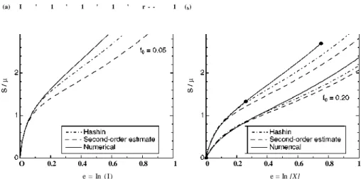
Figure 5. Nominal stress S = S _ n = S22 vs. logarithmic strain (e = l n ( A . ) in the case of in-plane

isotropic elongation (X = X\ = A,2).(a)/0 = 0.05. (b)/0 = 0.1 and 0.2. The exact solution of Hashin and of the second-order homogenization estímate are compared with the numerical simulations.

plotted in the following section are the averages of three-different realizations for each loading case. It is well known that averaging of various realizations improves the accuracy of the predictions for a given size of the RVE . It should be finally noted that RVEs were loaded in uniaxial tensión along two perpendicular directions to check their overall isotropy. The differences in the stress-strain curves were very small and similar to those obtained with different RVEs.

4. Results

The predictions of the homogenization model based on the second-order estimates with phase-field fluctuations developed by López-Pamiés and Ponte Castañeda were compared with the exact solution provided by the numerical simulation of an RVE for three different loading cases: isotropic tensile deformation, uniaxial tensile deformation and uniaxial traction. They were also compared in the first case with the exact solution derived by Hashin for a porous material whose microstructure was represented by the composite sphere assemblage model. The three loading cases were selected because they show large differences in triaxiality, and thus will serve to check the accuracy of the homogenization approach under very different loading scenarios.

4.1 In-plane isotropic deformation

The stress-strain curves corresponding to in-plane isotropic deformation are plotted in figure 5a for the porous elastomer with f0 = 0.05 and in figure 5b for those with

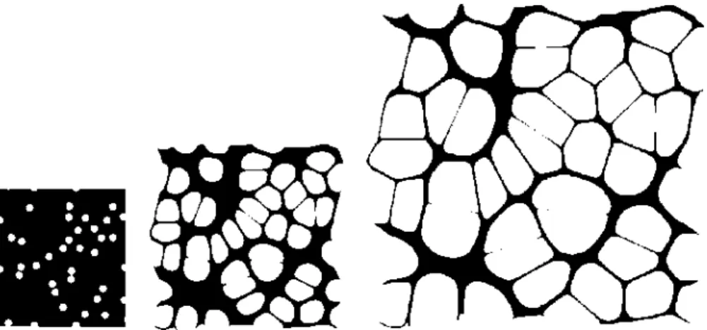
Figure 6. Evolution of the microstructure in the porous elastomer with/0 = 0.1 subjected to i n - p l a n e isotropic deformation. ( a ) X = l. ( b ) X = 1 .3 and ( c ) X = 2.3. T h e plots correspond to the solid circles in the stress—strain curve in figure 5(b).

stress in the plañe, S, was computed from the expressions for the effective strain energy of the porous elastomer (equations 9 and 18) as a function of the applied isotropic elongation X(= X\ = X2) as

As expected, the predictions of the homogenization models and of the numerical simulations are practically superposed in the small deformation regime for the three initial void volume fractions studied. Nevertheless, differences among the curves appeared afterwards, and they increased (and started at lower strains) as the initial volume fraction of voids decreased. The mechanical response provided by the numerical simulations was always the stiffest one, while the second-order estímate led to the most compliant behaviour. The origin of this divergence could be due to different assumptions between the numerical simulations and the homogenization models, and this point should be explored in further detail. For instance, Hashin's model provides an exact solution for the isotropic elastic deformation of a porous elastomer whose microstructure is given by the composite cylinder assemblage model. This void arrangement assumes a distribution in the voids radius while the numerical simulations were performed in RVEs with constant void radius. Obviously, the effect of monodisperse vs. polydisperse void radius is negligible for very small valúes of the void volume fraction and should be larger (and noticed at lower strains) as f0 increased. However, the trends found in figure 5 are exactly the

opposite, and the numerical and homogenization results tend to converge for larger valúes of the initial void volume fraction.

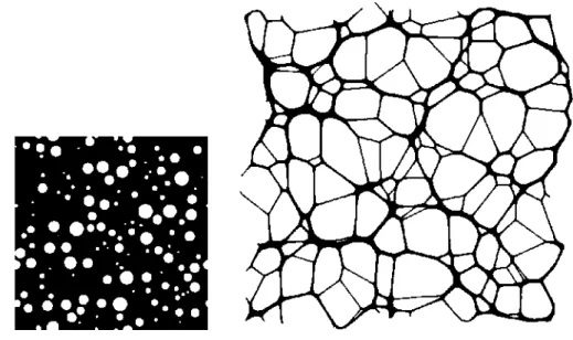
Figure 7. Evolution of the microstructure in the porous elastomer with /0 = 0.2 and_ a polydisperse pore size distribution subjected to in-plane isotropic deformation. (a)A = l. (b) A = 2.5

The three plots in figure 6 correspond to the solid circles in the stress-strain curve of the porous elastomer with/0 = 0.1 in figure 5b. It is evident from these plots that the circular pores do not remain circular during isotropic deformation, and the interaction between neighbouring pores leads to significant changes in the pore shape, which evolve towards polygonal shapes as the matrix ligaments between pores become thinner and are finally transformed into very thin struts which only carry load along their axes. It is interesting to notice that the divergence between the numerical and the homogenization models begins to be noticeable at X = 1.3, and the circular shape of the pores has been significantly altered at this level of deformation. The volume fraction of a monodisperse distribution of circular voids is limited and the spherical voids have to degenerate to a polygonal shape to accommodate the growth of the voids above this limit. However, the voids can remain circular in the particular case of the cylinder assemblage model, proposed by Hashin, which is based on a very particular microstructure (a polydisperse void distribution with an infinite gradation in pore size). In order to ascertain the influence of the void size distribution, an RVE was generated with fQ = 0.20 and a polydisperse void

distribution. The máximum pore radius in the model was that of the model with a constant void radius and fQ = 0.20 and the mínimum one was selected from the

condition that the discretization of the void perimeter included at least 12 elements. The microstructure was created using the random sequential adsorption algorithm, as in the monodisperse case, and the radius of each void was generated randomly between the máximum and mínimum void radius. Pores were added sequentially until the desired volume fraction (0.20) was reached and the final distribution is shown in figure 7a.

•/ ' /

1 /

/y

0.3

/ / / / / /

f0 = o.o5 / / 7 /

1 / yy /

/

s"

S*

/

/ y

•

SA

/ / I I s? y / i

I

Second-order estímate

Numerical

0.6 0.9

en = In(X-i) 1.2

f0 = 0.10

f0 = 0.20

1.5

Figure 8. Nominal stress Su vs. logarithmic strain en (=ln(Ai)) in the case of uniaxial

elongation (X2 = 1) for porous elastomers with different volume fraction of initial porosity/0. The predictions of the second-order homogenization estímate are compared with the numerical simulations.

voids vanished at large strains, as in the monodisperse case, and the final microstructure was polygonal, with a distribution of large and small polygons depending on the initial diameter of the corresponding pore. Moreover, the stress-strain curve was practically superposed to that of the monodisperse material in the whole range of deformation. These results indícate that the void size distribution (either monodisperse or polydisperse) played a minor role in the mechanical behaviour of porous elastomers because polygonalization of the microstructure to accommodate void growth occurred in both cases.

Finally, it should be noted that the second-order estímate with fluctuations developed by Lópéz-Pamiés and Ponte-Castañeda was superposed to the exact solution of Hashin for infinitesimal strains and underestimated the stiffness of the porous elastomer at finite strains. These differences were reduced as the initial porosity increased and both methods provide almost identical results w h e n /0> 0 . 3 ,

. This latter result - which could not be reproduced by homogenization approaches based only on the average fields in each phase - has demonstrated that the introduction of the effect of the field fluctuations is necessary to obtain the correct overall incompressible constraint in these materials

4.2 Uniaxial deformation

Uniaxial deformation (k\ A 0; X2 = 1) provides an intermedíate situation from the

viewpoint of triaxiality and constraint between the previous case of isotropic deformation and the next one of uniaxial tensión. The stress-strain curves corresponding to the second-order estímate were computed by differentiating the effective strain energy function given by equation (16) with respect to the uniaxial elongation X\. They are plotted in figure 7, together with the curves corresponding to the numerical simulations for porous elastomers with f0 = 0.05, 0.10 and 0.20. The

curves follow the general trends found for isotropic deformation: they are superposed in the small strain región, and divergences between numerical and homogenization results increase as the initial void volume fraction decreased. It should be noticed, however, that the differences were significantly smaller than in the case of isotropic elongation, and both curves were practically superposed in the whole deformation range explored in the case/o = 0.20.

The evolution of the microstructure under uniaxial elongation is shown in the plots of figure 9. The circular pores change progressively to polygonal domains, and the total porosity increases rapidly with deformation while the matrix ligament between neighbouring pores become thinner and thinner. However, the predictions of the second-order estímate with fluctuations are very cióse the exact numerical results regardless of the polygonal shape of the pores, as is shown in the case of the porous elastomer with/0 = 0.10 deformed up to X\ = 2.8. Noticeable differences were only found in the case of/o = 0.05 and they can be mainly attributed to the difficulties associated with modelling the incompressibility constraint (which is higher as the initial volume fraction of voids decreases) rather than to the polygonalization of the microstructure upon deformation.

4.3 Uniaxial traction

Uniaxial traction was simulated by deforming the porous elastomer along one direction (i.e. A,i^0) while the deformation in the perpendicular axis was unrestricted and 5 * 2 2 = 0. The triaxiality is thus reduced as compared with uniaxial deformation as well as the constraint in the deformation. The solution provided by the second-order estímate with fluctuations was obtained by solving numerically the equation (16) with the help of the program MATHCAD. For a given applied deformation X\,X2 was obtained from the set of equations

dW(XuX2)

-V- ' = 5 * 2 2 = 0 (21)

dx2 y '

r4v4 + r3v3 + r2v + rxv + r0 = 0. (22)

From the four different roots of v, only two roots are in the real domain if X\ ^í X2, and only the positive one can reproduce the uniaxial traction. Once X2 was

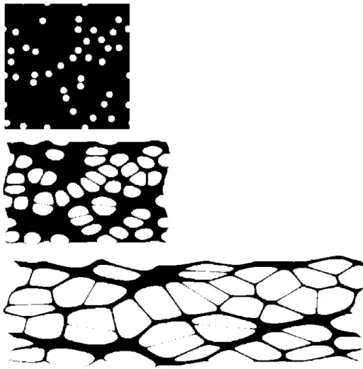
Figure 9. Evolution of the microstructure in the porous elastomer with/0 = 0.1 subjected to uniaxial elongation. (a) X\ = 1. (b) Ai = 1 . 3 and ( c ) X\ =2.8. The plots correspond to the solid circles in the stress-strain curve in 8.

fo = 0.05

f0 = 0.10

fo = 0.20

Second-order estímate

Numerical

Ó 0.3 0.6 0.9

en =\n(k~i)

1.2 1.5

Figure 10. Nominal stress Su vs. logarithmic strain eu (=ln(Ai)) in the case of uniaxial

traction (S22 = 0) for porous elastomers with different volume fraction of initial porosity f0.

The predictions of the second-order homogenization estímate [21] are compared with the numerical simulations.

Figure 1 1 . Evolution of themicrostructure in theporous elastomer with/0 = 0.1 subjectedto

uniaxial traction. (a) X\ = 1. (b) X\ =2.0 and (c) X\ =3.0. The plots correspond to the solid circles in the stress-strain curve in figure 10.

' i ' ' i ' ' —r—' ' 1 ' r

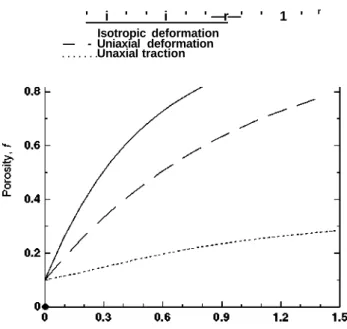
Isotropic deformation — - Uniaxial deformation

UnaxiaI traction

Figure 12. Numerical predictions for the evolution of the void volume fraction, /, in a porous elastomer with/0 = 0.1 subjected to in-plane isotropic deformation (X = X, = X2), uniaxial deformation(A = X\ X2 = 1) and uniaxial traction (X = X\ S22 = 0).

The differences in the pore shape between uniaxial traction and isotropic or uniaxial deformation are caused by the evolution of the porosity under these loading conditions. During deformation of a porous elastomer with an incompressible matrix, volumetric deformation can only be accommodated by void growth. Mathematically, this condition is expressed during plane-strain deformation (A3 = 1) by

f=l_l TJL (23)

A1A2

where k\ and A2 stand for the effective principal elongations. Porosity increases very rapidly during isotropic (Ai = A 2) and uniaxial deformation (A A 0 and A2 = 1), as

differences in the microstructure influence the stress distribution in the matrix. Máximum stresses are found in the thin matrix ligaments between polygonal voids, leading to large strain gradient in the matrix upon isotropic or uniaxial deformation, while stress variations are smoother when the microstructure maintains the original topology of ellipsoidal inclusions dispersed in the matrix.

It should be finally noticed that the simulations presented in this paper are limited to tensile loading modes. Compression of porous elastomers is also important from the fundamental and technological view-point, and the mechanisms of deformation are very different from those observed in tensión. The numerical simulation of the compressive deformation is hindered, however, by the development of local instabilities at the matrix ligaments between voids and it is difficult to obtain a numerical solution for large strains, which can be compared with the predictions of the homogenization models.

5. Conclusions

The finite deformation of porous elastomers was studied by means of the numerical simulation of an RVE of the microstructure. The size and the discretization of the RVE were selected to obtain an exact response (to a few percent) of the plane-strain deformation of a material made up of a random and isotropic dispersión of circular cylindrical voids embedded in an incompressible neo-Hookean matrix. Three different loading modes (in-plane isotropic elongation, uniaxial elongation, and uniaxial traction) were simulated, and the corresponding stress-strain curves as well as the evolution of the microstructure as a function of the applied deformation were presented for materials with an initial porosity of 5%, 10% and 20%.

These results can be very useful to check the accuracy of available homogeniza-tion for elastomeric materials and to point to the critical issues which should be addressed to improve the accuracy of the predictions. These possibilities were exploited by comparing the results with those given by two homogenization models for the finite deformation of porous elastomers. It was found that the solution for the in-plane isotropic deformation of a porous elastomer with circular pores derived by Hashin differed from the results obtained in materials with a monodisperse or polydisperse void distribution. Hashin's model assumes that voids remain spherical upon deformation and this is possible for the particular case of the composite assemblage model, with an infinite gradation in pore size, but not for other microstructures. The large volumetric strain during in-plane deformation has to be

with low initial porosity). They were mainly attributed to the difficulties associated with the accurate introduction of the incompressibility condition in the second-order homogenization estimates. In addition, the rapid change in the void morphology in these particular cases (from dispersed ellipsoids to large polygonal voids) to accommodate the volumetric strain by void growth has to be taken into account to provide precise information about the evolution of the microstructure in porous elastomers.

Acknowledgments

This investigation was supported by the Spanish Ministry of Education and Science through grant MAT 2006-2602 and by the Comunidad de Madrid through the program ESTRUMAT-CM.

References

R.A. White, F.M. Hirose, et al, Biomaterials 2 1 7 1 (1981). R. Langer and J.P. Vacanti, Science 260 920 (1993). T. Morí and K. Tanaka, Acta Metall. Mater. 21 571 (1973). R. H U Í , J. Mech. Phys. Solids 13 213 (1965).

R.M. Christensen and K.H. Lo, J. Mech. Phys. Solids 27 315 (1979). S. Torquato, J. Mech. Phys. Solids 46 1 4 1 1 (1998).

J. Segurado and J. LLorca, J. Mech. Phys. Solids 50 2107 (2002). P. Ponte Castañeda and P. Suquet, Adv. Appl. Mech. 34 171 (1998). J.L. Chaboche, P. Kanouté and A. Roos, Int. J. Plast. 21 1 4 0 9 (2005). C. González and J. LLorca, J. Mech. Phys. Solids 48 675 (2000). R. H U Í , Proc. Roy. Soc. London A 326 1 3 1 (1972).

N. Lahellec, F. Mazerolle and J.C. Michel, J. Mech. Phys. Solids 52 27 (2004). N. Triantafyllidis, M.D. Nestorovic and M.W. Schraad, J. Appl. Mech. 73 505 (2006). Z. Hashin, Int. J. Solids Struct. 21 711 (1985).

Q.-C. He, H. Le Quang and Z.-Q. Feng, J. Elast. 78 153 (2006).

O. López-Pamiés and P. Ponte Castañeda, Math. Mech. Solids 9 243 (2004). O. López-Pamiés and P. Ponte Castañeda, J. Mech. Phys. Solids 54 807 (2006). P.J. Blatz and W.L. Ko, Trans. Soc. Rheol. 6 223 (1962).

R. Abeyaratne and N. Triantafyllidis, J. Appl. Mech. 51 481 (1984). M. Danielsson, D.M. Parks and M.C. Boyce, Mech. Mater. 36 347 (2004). 0. López-Pamiés and P. Ponte Castañeda, J. Elast. 76 247 (2004). 1. Segurado, C. González and J. LLorca, Scripta Mater. 46 525 (2002). C. González, J. Segurado and J. LLorca, J. Mech. Phys. Solids 52 1573 (2004). 0. Pierard, J. LLorca, J. Segurado, et al, Int. J. Plast. 23 1041 (2007). 1. LLorca and J. Segurado, Mater. Sci. Engng. A365 267 (2004). I. Segurado and J. LLorca, Acta Mater. 53 4391 (2005). P. Ponte Castañeda, J. Mech. Phys. Solids 50 737 (2002). J.R. Willis, Adv. Appl. Mech. 21 1 (1981).