An experimental and numerical study of the pattern of cracking
of concrete due to steel reinforcement corrosion
B. Sanz3'*, J. P l a n a s
3, J.M. S a n c h obA B S T R A C T
In this work, cracking o f concrete due to steel reinforcement corrosion is experimentally and numerically studied. The tests combined accelerated corrosion—to generate the cracks—with impregnation under vacuum w i t h resin containing fluorescein—to enhance their visibility under ultraviolet light. In parallel, a model—called expansive joint element—WAS d e v e l o p e d to simulate the expansion o f the oxide and finite elements w i t h an e m b e d d e d adaptable cohesive crack w e r e used to describe concrete cracking. The results show that a g o o d agreement exists b e t w e e n the experimental and numerical crack patterns, w h i c h constitutes promising progress towards a comprehensive understanding of corrosion-induced cracking in reinforced concrete.
1. Introduction
Corrosion of steel reinforcement is one of the main pathologies of reinforced concrete structures. It involves generation of an oxide layer on the bar surface, which results in a decrease of the net cross-sectional area, thus, reducing its strength and decreasing the overall safety of the structure. However, long before a significant reduction in area is achieved, the volumetric expansion of the oxide induces internal pressure on the surrounding concrete, and leads to the cracking of concrete and, eventually, to full spalling of the cover [1-3].
Studying the evolution of the whole process requires an analysis of the transport of aggressive agents through the cover, determining the kinetics of the complex electrochemical phenomena occurring at the steel-concrete interface and predicting the mechanical effects of the expansive oxide layer on the surrounding concrete. This work concentrates on the last part of the process and compares the crack patterns observed in accelerated corrosion tests with the numerical crack patterns ob-tained from simulations, and is specially focused on assessing the ability of the numerical model to successfully simulate the cracking behavior observed in the experiments.
Nomenclature
0
tensorial product1 second order identity tensor
E elastic modulus
EoXi £ s t elastic moduli of the oxide and the steel
ft tensile strength of the concrete
CF fracture energy of the concrete
GF, fracture energy in the linear softening curve
Gox,
G
st shear moduli of the oxide and the steelCox
equivalent shear modulus of the oxide in the expansive joint elementh initial thickness of steel
stiffnesses of the expansive joint element
kn normal stiffness of the expansive joint element cut-off normal stiffness of the expansive joint element K„ stiffness tensor of the expansive joint element Km bulk modulus of the oxide
kt shear stiffness of the expansive joint element
k°t cut-off shear stiffness of the expansive joint element
n number of elements per quarter of the rebar circumference n unit normal to the corroding metal surface
N0X,Nst normal moduli of the oxide and the steel
K
x
equivalent normal modulus of the expansive joint element t traction vector acting on the metal surfaceu shear displacement resulting at the oxide surface Vox, Vst specific volumes of the oxide and the steel W crack opening width
w relative displacement vector in the expansive joint element W i characteristic crack opening of the linear softening curve
wm mechanical displacement (the difference of the total displacement and the displacement due to free expansion)
W t h threshold crack opening
X corrosion depth (amount of steel that is transformed into oxide)
Xo cut-off corrosion depth for the cut-off stiffness of the expansive joint element
a' adaption factor of the crack in concrete
P expansion factor of the oxide fix volumetric expansion of the oxide
n directionality factor of the expansive joint element
fit reduction factor of the normal tension stiffness of the expansive joint element V Poisson's ratio
V o x , Vs t Poisson's ratios of the oxide and the steel
0"/ maximum principal stress
T shear stress applied to the oxide surface
time through the corrosion current density. The expansive joint element is implemented within the finite element frame-work COFE (Continuum Oriented Finite Elements) and it frame-works together with finite elements with an embedded adaptable cohesive crack [6,7] which follow the basic cohesive model proposed by Hillerborg et al. [8] to simulate the fracture of con-crete and has been since used by many other researchers; see,e.g., [9-11] for details of the model and [12,13] for recent developments in the testing procedures to obtain the bilinear softening curve.
For the sake of better readabiliy, the paper is organized in a main text, in which the essential aspects of the experiments and simulations are described, and four appendices, in which further details of the model, the simulations, and the exper-iments are given. In the main text, Section 2 presents the experimental work and summarizes and discusses its results, Sec-tion 3 explains the numerical model, the simulaSec-tions and their results, and SecSec-tion 4 closes the main text with some final remarks and a list of conclusions.
2. Outline of the experimental study
2.1. Geometry of the specimens
cross-section of 100 x 90 m m2 and 90 m m in height, with a cast-in steel tube simulating a reinforcing steel bar of 20 m m
diameter and a cover of 20 mm, as shown in Fig. 1. The faces of the prism perpendicular to the axis of the tube w e r e covered w i t h an epoxy coating to induce essentially plane current and strain fields.
2.2. Specimen preparation
Concrete was manufactured w i t h Portland cement CEM I 52.5 R according to European Standard EN 197-1 [14]. Siliceous sand and aggregates w e r e used with a m a x i m u m aggregate size of 8 mm. Calcium chloride was added to the mixture to depassivate the steel. Set retarding admixture was also added to compensate for the accelerating effect of CaCl2. Table 1
dis-plays the mix proportion used.
The accelerated corrosion test specimens w e r e cast in steel molds with the appropriate holes to hold the steel tube in place. The protruding ends of the tube w e r e protected by an enamel coating to prevent corrosion.
The specimens w e r e removed from the molds after 24 h and stored, until testing time, in a bath of lime saturated water in a temperature-controlled chamber at 20 °C.
Six specimens, identified as A01-A06, w e r e cast and subjected to the tests described next.
2.3. Accelerated corrosion tests set-up
After curing, the samples w e r e surface dried, and a coating of epoxy resin was applied to the faces perpendicular to the tube axis. Simultaneously, the end of the tube that would be submerged in water during the test was covered with a PVC cap to provide electrical insulation of the portion of the tube protruding f r o m the concrete. Then the specimens w e r e placed in a water bath with the tube in vertical position and the level of water was adjusted to cover completely the lateral faces (see Fig. 2). A cylindrical shell of stainless steel surrounding the specimen was provided to act as the counter-electrode. Next, a constant current source was connected to the tube and to the counter-electrode, and an impressed current was applied to the system for the duration of the test. W i t h the precautions taken in insulating the top and bottom faces and the submerged end of the specimen, plane current f l o w and strain may be expected, resulting in nearly uniform corrosion depth along the length of the tube.
The duration of the corrosion and the current density w e r e selected to achieve relatively large crack openings (visible to the naked e y e ) in a time as short as possible. The impressed current density was set at 400 |jA/cm2, and the duration was
3 days, which, according to Faraday's law, should lead to a corrosion depth at the end of the test of 38 |j.m.
The applied current density of 400 |jA/cm2 is much higher than the values observed in real structures [15], which may
affect the type of oxide generated. However, this current density falls within the range 100-500 |j.A/cm2 for which Faraday's
law for steel dissolution has been shown to hold for chlorinated concrete [4,5]. The composition factor, which may affect the evolution of cracking with time, is not essential in the present study since the tests are only intended to assess the ability of the numerical model to capture the crack pattern.
2.4. Preparation of concrete slices to observe the crack pattern
After accelerated corrosion, the samples w e r e cut w i t h a low-speed radial diamond saw into slices to study the cracking along the bar and a grinding machine was used to improve the smoothness and parallelism of the surface of the cuts. W i t h that first treatment, the main cracks became visible and microcracks w e r e detected w h e n looked under a microscope.
In order to improve the detection of cracks, the slices w e r e impregnated under vacuum with resin containing fluorescein, a well known procedure to enhance crack visibility. The technique was implemented using a vacuum pump and a modified
C
>
• — 5 0 — • . 5 0 — • 9 0
-epoxy coating
1.0 mm thick steel tube
I Dimensions in mm
Fig. 1. Geometry of the specimens.
Table 1
Concrete mix proportions, by weight.
Water Cement Sand Aggregate CaCl, Set retarding Superplasticizer
electrical rebar (oxidation) source
H!
!i!
iii
counter electrode (reduction)
_ plain w a t e r
electrical insulation of
t h e bar: P V C cap
Fig. 2. Picture and sketch of accelerated corrosion tests assembly: an external electrical source supplies constant current to oxidize the bar, using a stainless
tube as counter electrode and plain water as conductor medium; the submerged end of the bar is electrically insulated by a PVC cap.
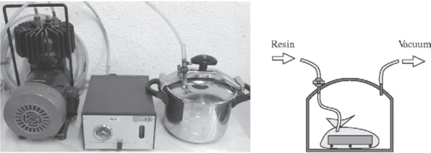
Fig. 3. Impregnation of the slices with low viscosity resin and fluorescein under vacuum: photo of the assembly (left), formed by—from left to right—a
vacuum pump, a vacuum/flow-meter and a modified pressure cooker; sketch of the impregnation chamber (right) with the vacuum outlet, the resin inlet, and a plastic bag containing the specimen and the resin.
pressure cooker as shown in Fig. 3 [16]. Before injection, the samples were dried at 105 °C until constant weight was achieved, according to ASTM standard C-642-90 [17] and, after that, vacuum was applied for 24 h to remove the air in the pores of the slices, reaching - 6 7 0 mmHg of manometric pressure. Then the resin was injected through one of the valves of the pressure cooker and, finally, the air was allowed back inside. After curing the resin at least for 24 h, the surface of the slices was ground again to eliminate the excess resin and to expose the base material.
A low viscosity resin was used, to facilitate the penetration of the resin into the micro-cracks and pores of concrete, and a concentration of 1.5 mg of fluorescein per milliliter of resin was selected among a set of five concentrations by choosing the smaller concentration that delivered good visibility of the mix under UV light. Complementary tests proved that the prep-aration process does not introduce spurious cracking in uncorroded samples (see Section D).
After the accelerated corrosion process, each specimen was cut into several slices, and two of them were impregnated according to the procedure described before. For specimen A01, two adjacent slices were impregnated, which provided three different specimen cross-sections for pattern inspection, at approximately 16 m m spacing. For specimens A02, A05 and A06, two non-adjacent slices were impregnated, which provided four different cross-sections, at approximately 20 m m spacing. For specimens A03 and A04, only one slice survived the process of preparation, so two cross-sections were available for inspection, separated approximately 20 m m from each other. A total of 19 cross-sections were photographed under natural light and under UV light after impregnation.
2.5. Experimental results
After the accelerated corrosion process, a single main crack was seen in all the specimens that ran through the cover roughly parallel to the axis of the tube. No other cracks were visible to the naked eye on the visible faces (those not covered with resin). However, secondary cracks were revealed when the slices of the specimens were examined, both under natural and UV light.
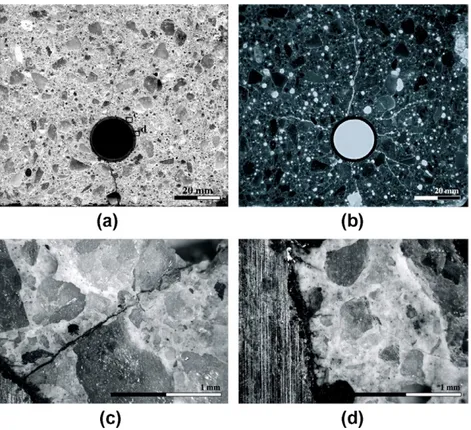
Fig. 4 shows four photographs of one of the cross-sections of specimen A01, which was selected for delivering one of the clearest UV pictures at the printer resolution for gray-shade scale.
(C) (d)
Fig. 4. Crack pattern in accelerated corrosion tests: general pattern viewed with the naked eye (a); general pattern of the slice after being impregnated
under vacuum with resin containing fluorescein and illuminated under UV light (b); detail of a secondary crack (c) at the position indicated by the upper small frame on Image (a); magnified v i ew of various radial micro-cracks ( d ) at the position indicated by the lower small frame on Image (a).
Magnified views at the locations marked by the t w o small rectangles are given below the wide-field images, which show thin secondary cracks, Fig. 4(c), and a f e w radial micro-cracks, Fig. 4(d). Bright vertical lines on the steel surface are observed, which were produced during the grinding process.
The image in Fig. 4(b) corresponds to the same slice photographed under UV light after impregnating it with resin and fluorescein, as described in Section 2.4. The secondary cracks are now clearly observable in the wide-field image without need for magnification.
An interesting observation is that the main crack, which is easily seen with the naked eye in the slice before impregnation, does not seem to have taken so much resin inside during the impregnation, probably because the crack is partially filled with compact black iron oxide; the same effect is observed at the root of the secondary cracks.
To assess the presence of iron oxide in the cracks, various slices that had not been impregnated with resin were split in t w o along the main crack and its diametrically opposite crack, as shown in Fig. 5. All of the split slices showed clear evidence
Fig. 5. Slice from specimen A01 split in t w o along the main crack and the diametrically opposite crack showing extended oxide layers within the main crack
of an extended oxide layer within the main crack and at the steel-concrete interface, while the oxide layer penetrated only slightly in the root of the opposite crack. Further research is necessary to disclose the transport mechanism of the oxide along the main crack. Since in the conducted tests the specimens w e r e submerged in water, one possibility is transport of dissolved ions—driven by the imposed electric field—along the channel provided by the crack, f o l l o w e d by progressive reaction of the moving ions to insoluble forms that w o u l d then precipitate on the surfaces.
W h e n the crack patterns of the remaining specimens w e r e examined, the visual perception was that they w e r e qualitatively very similar to that in Fig. 4(b), with a w i d e open main crack and several secondary cracks that irradiate f r o m the reinforcement towards the external boundary of the specimen without reaching its outer boundary. However, a closer observation reveals a very complex structure (see, e.g., the bifurcation of the t w o cracks in Fig. 4 ( b ) that emanate from the tube at about three and four o'clock). Indeed, the number of cracks in our experiments varied appreciably from one specimen to another, and even from a cross-section to another in the same specimen.
For an overall evaluation of the crack distribution, the visible cracks that emanate from the interface w i t h the steel w e r e examined for each of the 19 cross-sections; the total number of cracks identified is 108, and their distribution histogram is shown in Fig. 6. As can be seen, most of the cross-sections display 6 cracks, i.e., one main crack, and five secondary cracks. However, about one third of the cross-sections display 4, 5 or 7 cracks. The mean number of cracks is 5.7, with a relatively large standard deviation of 0.8.
W h e n the position of cracks in addition to their number was compared for all the specimens, it was found that the exact position and path of the cracks vary appreciably from one specimen to another, and even from a cross-section to another in the same specimen. To quantify this effect, the angular position of the root of each visible crack in each of the 19 resin-impregnated cross-sections was determined by superimposing the photograph of the section and a graduated circle, as shown in Fig. 7(a) for one of the cross-sections of specimen A04; the position of the crack at or near the steel surface was recorded to the nearest 5° on the inner graduated circle.
14
in 1 2
c o tS 10
03 to
£ 6 o
E
i 2
0
Fig. 6 . Crack histogram displaying the distribution of n u m b e r of cracks in each specimen cross-section.
(a) (b)
Fig. 7 . Polar plots of the m e a n angular position of the roots of the cracks at or near the steel surface: e x a m p l e ( s p e c i m e n A 0 4 ) of the superposition of the photograph of a section and a graduated circle used to measure the angular positions (a), and set of the polar plots f o r all the specimens (b). The a r r o w indicates the m e a n position of the main crack, and the symbols are as f o l l o w s : •— m e a n o f 4 crack positions out o f 4 sections; • — m e a n of 3 crack positions out of 3 sections; • — m e a n of 2 crack positions out of 2 sections; • — m e a n of 3 crack positions out of 4 sections; — m e a n of 2 crack positions out of 4 sections; + crack seen in only one section.
A01 Mean = 5.7
Std deviation = 0.9
A02
A04
A03 A02 A05 I
A06
3 4 5 6 7 8
Then the data w e r e processed to find the mean angular position of the root of each crack in each specimen, from which the polar plots shown in Fig. 7(b) w e r e generated. The position of a given crack in a given specimen varies from section to section with an overall standard deviation of 9°. This is equivalent to a length of about 1.6 m m along the circumference of the steel tube, which is well b e l o w the maximum aggregate size of the concrete. However, w h e n the position of the cracks in different specimens is compared, the exact position of the cracks—even that of the main crack—is so scattered that it is dif-ficult, if not impossible, to find a systematic correspondence b e t w e e n cracks other than the main crack. This is, again, attrib-utable to the intrinsic heterogeneity of concrete.
One could be tempted to push further the analysis of the impregnated samples and try to measure the crack lengths or crack openings. However, although no n e w cracks appear during the preparation process, the opening and visible length of the cracks may change during the process of cutting, drying and impregnating the slices (notably due to drying shrinkage). Thus, only the crack pattern is believed to be reliable, not the opening or length of the cracks.
3. Outline of the numerical simulations
The finite element simulations rest on t w o basic models: the cracking model, which is assumed to f o l l o w a cohesive crack behavior, and the oxide layer model, which is implemented as a layer of interface elements w i t h zero initial thickness which expand as the corrosion depth increases.
3.1. Model for the cracking of concrete
Fracture of concrete is modeled using the standard cohesive crack, introduced by Hillerborg et al. [8], In that model, the stresses in concrete are assumed to f o l l o w a softening curve that depends on the opening width of the crack. The cohesive behavior of concrete can be characterized in independent tests in which its fracture properties are determined by w e l l estab-lished procedures [12,13].
Concrete cracking is numerically modeled using a relatively simple implementation which combines constant strain ele-ments with an embedded cohesive crack w i t h limited adaptability [6,7]. The cohesive crack used in the element formulation is the simplest 3D extension of the standard cohesive crack under pure opening mode. It is fully characterized by a single scalar softening function, the same as for pure M o d e I crack growth, and the extension is based on the assumption that the forces are central, i.e., that the cohesive traction vector on one crack face is proportional to the relative displacement vector of the t w o crack faces.
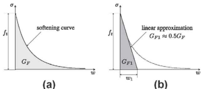
The softening curve presents a strong non-linearity, as shown in Fig. 8(a), but a linear approximation can be used in order to simplify or speed-up the calculations as depicted in Fig. 8(b). The linear approximation is fully defined by the tensile strength f of concrete and the characteristic crack width W]; the area Gfi under the linear curve is roughly one half of
the total fracture energy Gf [9].
The limited adaptability of the crack embedded in the element is actually a numerical expedient to avoid crack locking while keeping the formulation strictly local. It allows the crack to rotate to adapt itself to the local stress fields if the crack opening is smaller than a certain threshold wth, which, by default, is taken to be 0.2Gfi //t, in which Gfi and/t are defined in
Fig. 8(b). More generally, w e take the threshold to be
Wth = a ' w i ( 1 )
and call a' the adaptation factor of the embedded crack. Further details can be found in [6,7].
3.2. Model for the expansion of the oxide
The expansion of the oxide produced by a uniform oxidization of the reinforcement can be simulated by a pseudo thermal expansion of the steel bar. However, if perfect adherence b e t w e e n the steel and the concrete is assumed, the cracking is dis-tributed in the volume and no localized cracks appear until late stages of oxidization, w h e n high tensile stresses are reached
a, a,
ft
(a)
linear approximation / GFI « 0.5Gj?
(b)
w
Fig. 8. Standard cohesive model (a): when a crack is opening, stresses on the crack faces depend on the crack width according to the softening function
close to the outer surface of the concrete, as shown in Guzman's results f r o m independent calculations using the same type of finite elements used in the present w o r k [18,19].
To describe the actual behavior, it is essential to model the relative displacement b e t w e e n the concrete and the steel w h e n an oxide layer is formed b e t w e e n them. To do so, special interface elements are inserted b e t w e e n the steel and the concrete. Such interface elements, the so called expansive joint elements, incorporate both the expansion and the evolving mechanical properties of the oxide layer, as w e r e initially presented in [20]. Implementation of the elements was performed within the finite element framework COFE (Continuum Oriented Finite Elements), a particular finite element program written by the authors using C++ generic programming which provides high level constructs to define tensorial constitutive models. During the corrosion process, there is a layer of steel which is transformed into oxide; the thickness of such a layer is the
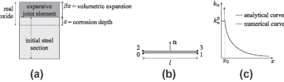
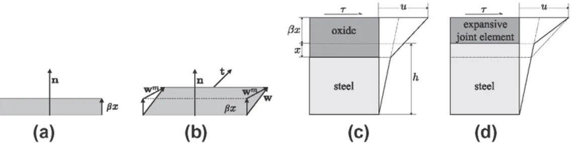
corrosion depth x, as sketched in Fig. 9(a). The loss of steel, however, is over-compensated by the oxidization because the spe-cific volume of the oxide is greater than the spespe-cific volume of the steel, resulting in a net expansion of the corroded layer of steel, as shown in Fig. 9(a). In order to simplify the calculations, the expansive joint element only includes the net volumetric expansion fix of the oxide while the steel section remains constant, as shown in Fig. 9(a); the composite behavior is obtained by a series-coupling model as described in detail in Section A.
The expansive joint element is a four-node element, with zero initial thickness, that models the g r o w t h of the oxide as an expansion perpendicular to the initial surface of the steel, which coincides with the line joining the nodes 0 and 1; g e o m e t -rically, the element is fully defined by the normal exterior to the steel surface n and by its length /, as depicted in Fig. 9(b).
The free volumetric expansion is assumed to depend linearly on the corrosion depth and on an expansion factor /i, which is defined by the ratio of the specific volumes of the oxide vox and the steel vst as
/» = 1 T - 1 ( 2 ) Vst
For a free expansion of the oxide, without any other mechanical actions, the traction vector t acting on the element is assumed to be zero. However, w h e n there is a mechanical displacement w apart f r o m the free expansion, the traction vector is calculated as
t = k„(w • n - fix)n + kt[w - ( w • n)n] ( 3 )
where n is the normal direction to the element and k„ and k, are, respectively, the normal and shear stiffnesses of the expan-sive joint element.
The composite stiffnesses k„ and k, are calculated to maintain mechanical equivalence of the real and the simulated sys-tems, based on the properties of the steel, the real oxide and the expansion factor /i, using a series coupling model.
From a simple analysis, it was found that the stiffnesses are inversely proportional to the thickness of the oxide layer and, thus, also to the corrosion depth, i.e.,
i 1 i 1
KN (X — , KT (X —
X X ( 4 )
which means that, as one might expect, the stiffness of the corrosion layer is infinite w h e n its thickness is zero.
To avoid numerical instabilities during the calculations for very small values of corrosion depth, a cut-off is set for a cer-tain corrosion depth x„, and the stiffnesses are taken as constant for corrosion depths smaller than x„, as shown in Fig. 9(c).
Thus, the numerical law for the normal stiffness is written as
k„ = if x < x0 ( 5 )
and a similar expression is obtained for the shear stiffness.
The model incorporates a debonding ability to allow easy relative m o v e m e n t of the steel and the concrete in shear and tension, which is necessary to achieve proper localization of the cracks. This is accomplished by taking a shear stiffness
fix = volumetric expansion
x = corrosion depth kl — numerical curve analytical curve
(a)
(b)
(c)
Fig. 9. Sketch of the expansive joint element: physical formation of oxide and modeling with the expansive joint element (a) and node-layout, length and
substantially less than the normal stiffness (k, - k„) and by strong directionality of the normal stiffness, implemented through a directionality factor i], which is equal to 1.0 for compression and much less than 1.0 for tension, i.e.,
~ \ r\t < 1 if w • n - fix > 0 ^
with Eq. (3) for the joint replaced by
t = i]kn(w • n - fix)n + fct[w - ( w • n)n] (7)
The formulation of the element is detailed in Appendix A, at the end of the paper. Currently, the oxide layer behaves elas-tically because no available data exist to support more sophisticated models.
3.3. Characteristics of the simulations
Table 2 displays the properties of the materials used in the computations. For steel, standard values were assumed, while the fracture parameters of concrete were determined from complementary tests.
For the oxide, no definitive experimental results are available, so, at this stage of the research, the values of the consti-tutive parameters of the oxide have to be assumed and should be verified in further studies. The expansion factor f} was ta-ken to be 1.0, as found in the literature [1,2,21], although other studies consider a greater expansion of the oxide [22,23]. For the normal stiffness, a wide range of values are found in the literature: in [2], the bulk modulus of the oxide was taken to be of the same order of magnitude as the bulk modulus of water (around 2 GPa); in [23,24] the elastic modulus was estimated from a combination of analytical models and experiments in which the radial displacement in concrete was measured by image correlation techniques; the values obtained in these t w o studies are, however, very different: an elastic modulus of 0.14 GPa is reported in [23] for an assumed Poisson's ratio of the rust of 0.2, while the values of the elastic modulus reported in [24] range between 2 and 20 GPa, and no reference to Poisson's ratio was made by the authors. In the present paper, a fluid-like behavior is assumed, similar to that proposed by Molina, Alonso and Andrade in [2], with bulk modulus of rust of 2 GPa, and a vanishing small shear modulus; a f e w calculations were also run with bulk modulus equal to 0.2 GPa, and to 20 GPa, to test the sensitivity of the results to large variations of this parameter (see Section A for the details). The remain-ing parameters, x0l k°t and i]t, were chosen as small as possible—to achieve debondability as described in Section B—while
keeping the computations stable.
Simulations were carried out on 2D FE models of the specimens described in Section 2.1, except that a bar was used in-stead of a tube. The mesh was generated using the pre-post Finite Elements mesh processor Gmsh [25] and constant strain triangles were used for the steel and concrete elements. The boundary conditions of the problem were t w o simple supports at the base of the concrete section. The calculations were driven by the corrosion depth x, from which the free radial expan-sion fix was computed at each step.
Four meshes were used to check if the results are mesh insensitive, with refinements of 4, 8,16 and 32 interface elements per quarter of circumference (roughly equivalent to element sizes of 4, 2, 1 and 0.5 mm, respectively). The size of the ele-ments of concrete at the outer boundary was set equal to five times the length of the eleele-ments at the steel-concrete inter-face. Appendix C summarizes the essential aspects of the comparison.
A total radial expansion of 20 |j.m was applied in 40 steps, which, although considerably less than the expansion reached in the tests, was enough to produce a stable pattern of localized cracks. The computational limitation comes from the known fact that when the (numerical) crack tip approaches a free surface in bending mode (i.e., with a compression zone ahead of the crack tip), as happens with the longest secondary crack in the present geometry, it tends to curl over itself and to block due to excessive gradients. However, as pointed out before, for an expansion of 20 |j.m the simulations already show a well defined and stable crack pattern, which can be confidently used to be compared with those seen in the experimental results.
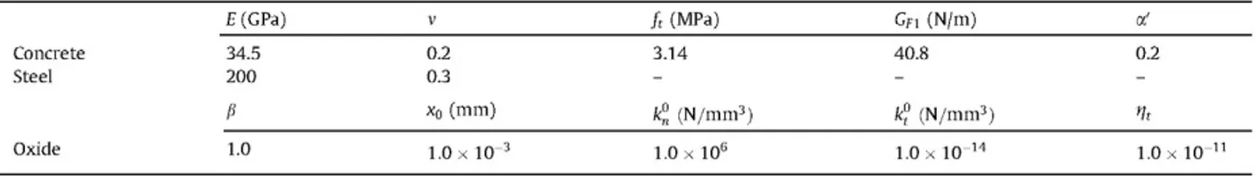
3.4. Results of the numerical simulations
Fig. 10 shows the distributions of maximum principal stress, cracks, and crack widths at various loading steps, illustrating the evolution of the process up to a final radial expansion of 20 |j.m. The results correspond to a mesh in which 8 cohesive
Table 2
Mechanical properties of the materials, where E is the elastic modulus, v is Poisson's ratio, f, is the tensile strength, GFI is the fracture energy bellow the linear
softening curve, a' is the adaption factor of the crack, p is the volumetric expansion factor, x0 is the cut-off corrosion depth, fcj and k° are the cut-off normal and shear stiffnesses and is the reduction factor of the normal tension stiffness.
E (GPa) V f, (MPa) GF, (N/m) a!
Concrete 34.5 0.2 3.14 40.8 0.2
Steel 200 0.3 - -
-P x0 ( m m ) k°n ( N / m m3) k° ( N / m m3) >lt
w (mm)
0 0
sigma_l (MPa)
1.57 ;
x = 3 pm
w (mm)
0.0188
sigma_l (MPa)
1.57 3.14
x = 7 pm
w (mm)
0.0241
sigma_l (MPa)
1.57 3.14
x = 9 pm
w (mm)
0.0522
sigma_l (MPa)
1.57 3.14
x = 20 (jm
Fig. 10. Crack pattern and map of tension stresses obtained in numerical simulations using the expansive joint element at corrosion stages of 3, 7, 9 and
20 |im, w i t h w being the crack opening w i d t h in millimeters and a, the m a x i m u m principal stress.
elements were inserted per quarter of circumference (equivalent to an element length of about 2 mm). The stress scale is in MPa with positive values corresponding to tension (white) and negative values to compression (black); the scale for the crack width is in millimeters.
When the expansion begins, the tensile stress increases in the concrete elements, until the tensile strength is reached and, then the first cracks appear. At very early stages of corrosion, a cloud of finely spaced radial cracks of similar extent appears around the steel bar, but soon, for 3 |j.m of radial expansion, one of the cracks jumps to the concrete surface (see the image corresponding to x = 3 |j.m in Fig. 10). Although, according to the legend, the crack width appears to be zero, this actually means that the embedded cracks are still free to reorient because their width is less than the threshold value for consolida-tion wth, which is equal to 2.6 |j.m according to the parameters in Table 2.
After a f e w more steps (x = 7 |j.m), the main crack is consolidated (i.e., further rotation of the embedded crack is pre-vented), its maximum opening has increased up to 37.6 |j.m, the elements surrounding it have unloaded, and the nearest cracks are partially closed; on the other side of the steel bar, the zone of high tensile stresses (white area) has expanded as well as the cloud of radial cracks, although none has localized yet.
As the expansion increases further (x = 9 |j.m), some of the radial cracks begin closing and the localization of the upper central, vertical crack becomes apparent. Localization continues until, for the last corrosion step (x = 20 |j.m), the cloud of radial cracks has disappeared and five long secondary cracks become clearly defined. At this step, the opening of the main crack at its root (close to the steel) is approximately equal to the diametral expansion of the oxide, i.e., about 40 |j.m, and its maximum opening is 104 |j.m.
The results of the computations carried out for Gox = 0.2 GPa and Gox = 20 GPa, turned out to differ less than 2.6% and
5.5% respectively from the results of the computations reported here (Gox = 2 GPa), which indicates a low sensitivity of
the results to changes in the value of the bulk modulus of the oxide.
main crack and 3 - 5 secondary cracks depending on the mesh: 3 for the coarsest mesh, 4 for the t w o finer meshes and 5 for the mesh used in most of the verifications. In v i e w of the important simplifications considered in the modeling, the numer-ical predictions seem to be consistent with the experimental findings of 4.7 secondary cracks, on average.
4. Conclusions
The foregoing results show that a good agreement exists between the crack pattern obtained in accelerated corrosion test and those predicted numerically, which constitutes promising progress towards a comprehensive understanding of corro-sion-induced cracking in reinforced concrete. In particular, the following conclusions can be drawn:
• The crack pattern caused by oxide expansion is clearly revealed when specimen slices are impregnated under vacuum with resin containing fluorescein and subsequently inspected under UV light.
• The process of impregnation does not produce noticeable cracks on the samples, as tested on slices cut from specimens not subjected to accelerated corrosion.
• For the geometry under study, the resulting pattern consists of a single, wide open main crack and between three and six secondary cracks with a predominance of five secondary cracks (63% of cross-sections).
• The mean number of secondary cracks per cross-section is 4.7, with a standard deviation of 0.8.
• Although the subjective visual impression is that the crack patterns are "similar", the actual position of the cracks is highly scattered and no quantitative correlation can be easily established between the positions of the cracks in the whole set of experiments. The scatter is thought to be due to the heterogeneity of concrete.
• The proposed expansive joint element, endowed with the debondability property described in the paper, provides an ade-quate means to describe the oxide expansion.
• The combination of finite elements with an embedded adaptable cohesive crack (which describe the cracking of concrete), together with expansive joint elements, leads to crack localization in a manner similar to that found experimentally, with three to five secondary cracks depending on the mesh.
• The numerical method seems to be free of spurious mesh sensitivity as long as global (in the sense of integral or averaged) variables are concerned, notably, the main crack mouth opening.
• The details of the crack pattern do depend on the mesh. Indeed, the mesh is believed to introduce, in an otherwise homo-geneous continuum, the (spurious) heterogeneity that ultimately leads to the transition from highly distributed cracking to fully localized cracks.
Although this work was deliberately limited to the study of crack patterns, it is thought to provide a reasonable evidence that combining relatively simple experimental techniques with conceptually straightforward numerical models provides a powerful methodology towards disclosing the mechanisms of corrosion-induced cracking.
The results show that the predicted crack pattern is rather insensitive to some of the mechanical parameters of the oxide layer. This means that further work is necessary to narrow the interval in which the mechanical parameters of the oxide lie; work is in progress to find methods to quantify the expansion ratio of the oxide and the stiffness and strength of the rust layer.
Acknowledgements
The authors gratefully acknowledge the Secretaria de Estado de Investigacion, DesarroIIo e Innovacion of the Spanish
Min-isterio de Economia y Competitividad for providing financial support for this work under grant BIA2010-18864.
Appendix A. Formulation of the expansive joint element
Consider an expansive joint element as depicted in Figs. A l l ( a and b), with unit normal to the metal surface n, and let w be the relative displacement between the t w o faces of the expansive joint element, and t the traction vector acting on the side of the element in contact with the concrete.
When the oxide is freely expanding, i.e., when t = 0, the relative displacement vector is assumed to be normal to the me-tal surface, as shown in Fig. A l l ( a ) , and thus w = fixn.
In a general case, when external actions are simultaneously applied to the joint, the traction vector can be assumed, as a first approximation, to be linearly related to the mechanical displacement vector wm, which is defined in Fig. A . l l ( b ) and is
the difference of the total displacement and the displacement due to free expansion:
t = K„wm with wm = w - flxn ( A . l )
where K„ is a second order stiffness tensor that explicitly depends on the unit normal n. Objectivity behavior for a change of observer is required, so the tensor K„ should be objective and thus, if the surface is isotropic, it can be expressed as follows:
• y
^ - r f f i
r U j T . u
1
fix oxide expansive
joint element
/x/
/
h
7/
steel h steel
/
(a)
(b)
(c)
(d)
Fig. A.11. Stresses and displacements in the expansive joint: free expansion (a); traction vector, relative displacement and mechanical displacement (b);
displacement law resulting from the application of a shear stress to the real section (c); displacement law when the expansive joint is used (d). The stiffnesses of the expansive joint element are calculated so that the mechanical behavior is equivalent in the real and simulated systems.
where 1 is the second order identity tensor, ® indicates tensorial product of two vectors and kt and k2 are stiffness constants.
It is convenient to split the tensor K„ in its normal and shear components as follows:
K„ = k„n o n + fct(l - n o n) (A.3)
where k„ and kt are the normal and shear stiffnesses, respectively. Substituting the latter equation into Eq. (A.l), the
follow-ing expression is obtained:
t = k„(w • n - fix)n + kt[w - ( w • n)n] (A.4)
To take into account that the expansive joint concentrates the deformation of the oxide in a layer thinner than the actual oxide layer, the stiffnesses of the expansive joint element k„ and k, should be calculated to obtain a mechanical effect in the simulated system equivalent to the actual one. Let us consider, for simplicity, the case in which a pure shear stress T is ap-plied to the surface of the actual oxide layer, as shown in Fig. A.l 1(a). It produces a total shear displacement u at that surface, which is given by the sum of the shear displacement of the steel layer plus that of the oxide layer, which is expressed as
u = ( h - x )7l + ( l + / ? ) xJJ - (A.5)
where Gst and Gox are, respectively, the shear moduli of the metal and oxide and h is the initial thickness of steel, before the
corrosion started. For the same stress T, the displacement is calculated in the simulated section, using the expansive joint element, which keeps constant the thickness of the steel layer:
u T
u = h — (jst
T
(A.6)
with G*x being the equivalent shear modulus of the expansive joint element. Imposing that the displacement u must be the
same in both cases, the following expression for G*x is found:
G„v — j n + / ? ) _ r Gst.
and then the shear stiffness kt is calculated as:
k - G°x
(A.7)
(A.8)
The same reasoning is done under the hypothesis of uniaxial tension, obtaining a similar relation for the normal modulus
Nnx and the normal stiffness k„ of the expansive joint element:
k
l<n ~ px with N* = ,
n + fl
N„:
J _
Nst (A.9)
where Nox and Nst are the normal moduli of the oxide and the steel, respectively.
Unfortunately, the normal moduli depend on the lateral confinement and on Poisson's ratio v. For unconfined uniaxial loading or v = 0 the normal moduli coincide with the elastic moduli. For fully confined behavior, the normal moduli are gi-ven in terms of elastic moduli and Poisson's ratios by
1 - V0 X „ 1 - V s t r
Nox =
( 1 + vo x) ( l - 2 vo x)
N st =
( l + vs t) ( l - 2 vs t)
(A-10)
If the oxide is assumed to be in the form of a gel behaving like a liquid, as assumed by Molina et al. in [2], then Nox coincides
No x = ^ox, co x = 0 (A.11)
Since, according to the values found in the literature, the stiffness of the oxide layer might range from 0.1 to 0.001 times that of the steel, Eq. (A.9) can be approximated as
N o x (A.12)
(1 + p)x
and a similar approximation can be used for the shear stiffness.
From the preceding equation, it turns out that the stiffnesses of the expansive joint element are inversely proportional to the corrosion depth x, so for x —> 0, l<„ and kt —> oo. To avoid numerical instability, cut-off stiffnesses k°n and k°t are stablished for a certain small value of corrosion depth x0, and so, w e write
for x > x0 : kt = k° ^ and l<„ = k° ^
A further refinement is introduced in the model to allow the interface to behave differently in tension and in compression, which, as shown in the next appendix, is necessary, to achieve proper localization of the cracks in the neighborhood of the steel. This is accomplished by a directional factor i], which is equal to 1.0 for compression and much less than 1.0 for tension:
f l i f w n - i S x s j O ,A i y i
il = < r (A.14)
' I r\t < 1 if w • n - fix > 0 y
with Eq. (A.4) for the joint replaced by
t = i]k„(w • n - fix)n + k,[w - ( w • n)n] (A.15)
Appendix B. Debonding ability of the model
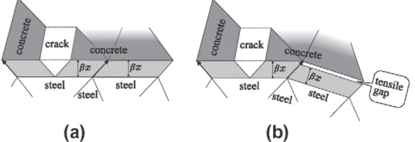
When perfectly elastic behavior of the oxide layer is assumed, with relatively high bulk and shear moduli, a nearly perfect bond behavior is achieved, which implies that crack localization is prevented: a cloud of finely spaced radial cracks, with very small opening at its point of intersection with the steel spreads through the concrete. Since the experimental results show that radial cracks do open significantly at their intersection with the oxide layer, the shear stiffness needs to be significantly reduced to reproduce the experimental effect. In fact, w e adopt here the view of Molina et al. [2], and model the rust layer as a quasi-fluid, with a shear modulus Gox = 10~8 x Kox.
A low shear modulus improves the results, but the cracks are not still completely free to open, except when the interface of the concrete and the steel is plane, as shown in Fig. B.12(a) which represents the rigid body kinematics of a crack that crossed a concrete element in contact with an expansive joint element (leftmost element). The crack opening induces shear on the interface and on its right neighbor (the left neighbor is not drawn), but since the shear modulus is very small, this does not induce any significant forces opposing the opening of the crack. However, when the surface of the steel is curved, the t w o neighboring interfaces are at an angle, however small, as shown in Fig. B.12(b), and when the crack opens, the pure shear in the first interface element induces a normal extension in the neighboring interface, shown as tensile gap in the figure. Thus, compatibility requires a normal tension to appear on the elements on each side of the cracked one. If the tensile normal stiff-ness is as high as the compressive stiffstiff-ness, this induces significant forces opposing to the crack opening. This is why w e need to introduce the directionality factor i/ described in Eqs. (A.14) and (A.15).
To show that effect, simulations were carried out on 2D FE models of the specimens described in Section 2.1 (except that a bar was used instead of a tube) and using the material properties shown in Table 2, first without considering the
t
w (mm) s i g m a j (MPa) w (mm) sigma_l (MPa) 0 0.0235 0.047 -6.8 19.4 45.6 0 0.0266 0.0532 -6.26 -1.48 3.3
Fig. B.13. Influence of the tension stiffness on the crack opening w i d t h w and m a x i m u m principal stress a,, w h e n simulating a radial expansion of 10 |im:
m o d e l i n g of the o x i d e w i t h reduced shear stiffness but high tension stiffness ( l e f t ) and m o d e l i n g o f the o x i d e w i t h reduced shear and tension stiffnesses (right).
directionality factor, i.e., considering a same stiffness in tension and compression, and then activating the directionality fac-tor, thus, strongly reducing the stiffness in tension. Fig. B.13 shows the results for a radial expansion of 10 |j.m.
In the simulation case that does not consider the directionality factor (left), the main crack has formed, but a close look at the results shows that the root of the main crack is clamped at the steel surface, and, as a consequence, a strong tensile stress concentration develops near the crack root, which is clearly visible as t w o white elements, one in the steel and the other in the concrete near the root of the crack.
When the stiffness in tension is reduced by the directionality factor i]t (see Eq. (A.14)), simulating a kind of debonding, the
stress lock-in is completely relieved, as seen in Fig. B.13 (right). There is a better localization of cracks for the same corrosion level: the nearest cracks to the main crack have mostly closed and the opening width of the main crack at the steel surface is
n = 16 n = 32
0 . 0 5 2 0.104
Fig. C.14. Effect of the m e s h size on the crack pattern, for a radial expansion of 20 |im and meshes of 4, 8, 16 and 32 elements of oxide per quarter of
nearly twice the total radial expansion applied (the total diametral expansion). The point of stress concentration disappears and all the elements in the steel are in compression, then the highest value of tension corresponds to the tensile strength of concrete. Also the values of compressive stress diminish.
Appendix C. Influence of the mesh size
To study the influence of the mesh size, simulations w e r e carried out using four meshes w i t h refinements of 4, 8 , 1 6 and 32 interface elements per quarter of circumference (roughly equivalent to element sizes of 4, 2, 1 and 0.5 mm). For all the meshes, the size of the elements of concrete at the boundary was set equal to five times the length of the elements at the steel-concrete interface.
Fig. C.14 shows the crack pattern obtained for a radial expansion of 20 |j.m for each mesh, and Fig. C.15 displays the evo-lution of m a x i m u m crack opening versus the corrosion depth for each mesh size. In all the cases, a main crack developed through the concrete cover, with an opening at the root of the crack roughly equal to the diametral expansion, and several secondary cracks appeared around the steel bar, each with a very small opening. The number of secondary cracks ranges b e t w e e n four and five, except for the coarsest mesh, which only has three secondary cracks; that mesh might be too rough to properly reproduce the cracking, as there are only five elements of concrete at the boundary, which explains the difference
Crack opening width versus corrosion depth
— ^ n 0 4 - - = - n 0 8 — — n 16 —« — n 32 — ^ n 0 4 - - = - n 0 8 — — n 16 —« — n 32
0 0.005 0.01 0.015 0.02
x (mm)
Fig. C . 1 5 . Effect o f the m e s h size on the m a x i m u m crack w i d t h : the m a x i m u m crack opening w i d t h w versus the corrosion depth x is s h o w n f o r meshes o f 4, 8 , 1 6 and 32 elements o f o x i d e per quarter of circumference.
in the number of cracks and which may result in an early locking at the secondary cracks, affecting to the curves of crack width for advanced stages of expansion. The curves of evolution of maximum crack opening are very close to each other for all the meshes, especially for the three finer meshes.
Appendix D. Evaluation of the damage produced by the procedure of impregnation
To demonstrate that the process of impregnation of the slices under vacuum does not introduce any noticeable crack in them, the slices cut from t w o specimens no subjected to accelerated corrosion were impregnated in the same manner as those coming from corroded samples, i.e., (1) the samples were cut into slices, ( 2 ) the surface of the slices was ground, (3) the slices were dried in an oven, ( 4 ) then impregnated under vacuum with resin, and ( 5 ) the surface of the slices was ground again to eliminate the excess resin. The inspection of the slices under UV light confirmed that no cracks were pro-duced during the impregnation of the samples. A picture of one of the slices is shown in Fig. D.16, showing no noticeable cracks.
References
[1] Andrade C, Alonso M, Molina F. Cover cracking as a function of bar corrosion: Part I - Experimental test. Mater Struct 1993;26:453-64.
[2] Molina F, Alonso M, Andrade C. Cover cracking as a function of bar corrosion: Part II - Numerical model. Mater Struct 1993;26:532-48.
[3] Alonso M, Andrade C, Rodriguez J, Diez J. Factors controlling cracking of concrete affected by reinforcement corrosion. Mater Struct 1997;31:435-41.
[4] El Maaddawy T, Soudki K. Effectiveness of impressed current technique to simulate corrosion of steel reinforcement in concrete. J Mater Civil Engng 2003;15:41-7.
[5] Care S, Raharinaivo A. Influence of impressed current on the initiation of damage in reinforced mortar due to corrosion of embedded steel. Cem Concr Res 2007;37:1598-612.
[6] Sancho JM, Planas J, Cendon DA, Reyes E, Galvez JC. An embedded cohesive crack model for finite element analysis of concrete fracture. Engng Fract Mech 2007;74:75-86.
[7] Sancho JM, Planas J, Fathy AM, Galvez JC, Cendon DA. Three-dimensional simulation of concrete fracture using embedded crack elements without enforcing crack path continuity. Int J Numer Anal Methods 2007;31:173-87.
[8] Hillerborg A, Modeer M, Petersson P. Analysis of crack formation and crack growth in concrete by means of fracture mechanics and fracture elements. Cem Concr Res 1976;6:773-82.
[9] Bazant Z, Planas J. Fracture and size effect in concrete and other quasibrittle materials. Boca Raton (FL): C.R.C. Press; 1998.
[10] Elices M, Guinea GV, Gomez J, Planas J. The cohesive zone model: advantages, limitations and challenges. Engng Fract Mech 2002;69:137-63.
[11] Planas J, Elices M, Guinea GV, Gomez FJ, Cendon DA, Arbilla I. Generalizations and specializations of cohesive crack models. Engng Fract Mech 2003;70:1759-76.
[12] Planas J, Guinea GV, Galvez JC, Sanz B, Fathy AM. Experimental determination of the stress-crack opening curve for concrete in tension. Report 39. Chapter 3. Indirect tests for stress-crack opening curve, Technical report, RILEM TC 187-SOC Final Report; 2007.
[13] Fathy AM, Sanz B, Sancho JM, Planas J. Determination of the bilinear stress-crack opening curve for normal- and high-strength concrete. Fatigue Fract Engng M 2008;31:539-48.
[14] European Standard for Cement - Part 1: Composition, specifications and conformity criteria for common cements EN-197-1; 2011.
[15] Andrade C, Alonso C, Rodriguez J, Garcia M. Cover cracking and amount of rebar corrosion: importance of the current applied in accelerated tests. In: Concrete repair, rehabilitation and protection, R.K. Dhir and M.R. Jones, EFN Spon, London, UK; 1996. p. 263-73.
[16] Sanz B, Planas J, Sancho J. Comparison of the crack pattern in accelerated corrosion tests and in finite elements simulations. Anal Mech Fract 2010.
[17] ASTM (Ed.), Standard test method for specific gravity, absorption, and voids in hardened concrete, C-642-90; 1990.
[18] Guzman S, Galvez JC, Sancho J. Cover cracking of reinforced concrete due to rebar corrosion induced by chloride penetration. Cem Concr Res 2011;41:893-902.
[19] Guzman S, Galvez JC, Sancho J. Modelling of corrosion-induced cover cracking in reinforced concrete by an embedded cohesive crack finite element. Engng Fract Mech 2012;93:92-107.
[20] Sanz B, Planas J, Fathy AM, Sancho JM. Modelizacion con elementos finitos de la fisuracion en el hormigon causada por la corrosion de las armaduras. Anal Mech Fract 2008;25:623-8.
[21] Michel A, Pease BJ, Geiker M R Stang H, Olesen JF. Monitoring reinforcement corrosion and corrosion-induced cracking using non-destructive X-ray attenuation measurements. Cem Concr Res 2011;41:1085-94.
[22] Bhargava K, Ghosh AK, Mori Y, Ramanujam S. Model for cover cracking due to rebar corrosion in RC structures. Engng Struct 2006;28:1093-109.
[23] Care S, Nguyen Q.T, L'Hostis V, Berthaud Y. Mechanical properties of the rust layer induced by impressed current method in reinforced mortar. Cem Concr Res 2008;38:1079-91.
[24] Pease BJ, Michel A, Thybo A, Stang H. Estimation of elastic modulus of reinforcement corrosion products using inverse analysis of digital image correlation measurements for input in corrosion-induced cracking model. In: 6th International conference on bridge maintenance, safety and management (IAMBAS), Lake Como, Italy; 2012.