Dealing with inaccurate face detection for automatic gender recognition with partially occluded faces

Texto completo

(1)Dealing with Inaccurate Face Detection for Automatic Gender Recognition with Partially Occluded Faces? Yasmina Andreu, Pedro Garcı́a-Sevilla, and Ramón A. Mollineda Dpto. Lenguajes y Sistemas Informáticos Universidad Jaume I. Castellón de la Plana, Spain. {yandreu, pgarcia, mollined}@uji.es Abstract. Gender recognition problem has not been extensively studied in situations where the face cannot be accurately detected and it also can be partially occluded. In this contribution, a comparison of several characterisation methods of the face is presented and they are evaluated in four different experiments that simulate the previous scenario. Two of the characterisation techniques are based on histograms, LBP and local contrast values, and the other one is a new kind of features, called Ranking Labels, that provide spatial information. Experiments have proved Ranking Labels description is the most reliable in inaccurate situations.. 1. Introduction. Over the past decades, a great number of papers have been published in the face analysis area. Most of them dealt with face recognition [1, 2] and face detection [3–6] problems. However, automatic gender classification has recently become an important issue in this area. Gender recognition has applications in several fields, such as, in demographic data collection, and it also could be an interesting starting point for other face image processes. According to recent papers [3, 4], face detection tasks obtain quite impressive results, although they do not reach 100% accuracy in all situations. Moreover, faces could be occluded by pieces of cloth, such as, scarves or glasses. Consequently, we will focus on the gender recognition problem when the face is not accurately detected and only a partial view of the face is available. In this paper, we compare several characterization techniques in order to find out which one performs better with the previous restrictions. All these techniques consider a set of N ×N windows over each face image. A feature vector is extracted from each individual window in order to characterize the face. The techniques used are: a well-know method based on Local Binary Patterns (LBPs) which have achieved good results in the face recognition task [2], a description based on Local Contrast Histograms (LCH) which can be used independently or together with the LBP [7] and the features proposed by the authors that have ?. This work was partially funded by Projects Consolider Ingenio 2010 CSD2007-00018, DPI2006-15542, and AYA2008-05965-C04-04 from the Spanish Ministry of Science and Innovation, and P1-1B2007-60 from the Fundació Caixa Castelló-Bancaixa..

(2) been specifically designed to keep not only the contrast information but also the positional information of each pixel inside its window [8]. The rest of the paper is organized as follows: the face descriptions used are introduced in Section 2; in Section 3, the experimental set-up is described in detail; in Section 4, the results are shown and discussed. Finally, our conclusions are given in Section 5.. 2. Face descriptions. This section presents all the face characterization methods used in the experiments, including our features called Ranking Labels. All the face descriptions use a window that scans the face image to obtain the feature vectors that will characterize the corresponding face. Two of the characterization methods considered are based on histograms computed over the image window (LBP and LCH) while the other method assigns a label to each pixel in the window in such a way that it keeps the information about the position of the pixels inside it. 2.1. Local Binary Patterns. The LBP operator was originally defined to characterize textures. It uses a binary number (or its equivalent in the decimal system) to characterize each pixel of the image. In the most basic version, to obtain this number, a 3 × 3 neighborhood around each pixel is considered. Then, all neighbors are given a value 1 if they are brighter than the central pixel or value 0 otherwise. The numbers assigned to each neighbor are read sequentially in the clockwise direction to form the binary number which characterize the central pixel. The texture patch in a window is described by the histogram of the LBP values of all the pixels inside it. To deal with textures at different scales, the LBP was extended to use neighborhoods of different radii. The local neighborhood is defined as a set of sampling points spaced in a circle centered at the pixel to be labeled. A bilinear interpolation is used when a sample point does not fall in the center of a pixel. In the following, the notation LBPP,R will be used to refer to LBP that uses a neighborhood with P sample points on a circle of radius R. The LBP operator can be improved by using the so-called uniform LBP [9]. The uniform patterns have at most two one-to-zero or zero-to-one transitions in the circular binary code. The amount of uniform LBP (LBPu ), when a 8neighborhood is considered, is 58. However, a histogram of 59 bins is obtained from each window, since the non-uniform patterns are accumulated into a single bin. Although the number of patterns is significantly reduced from 256 to 58; it was observed that the uniform patterns provide the majority of patterns, sometimes over 90%, of texture [10]. The LBP operator gives more significance to some neighbors than to others, which makes the representation sensitive to rotation. In order to obtain a LBP rotationally invariant [9], all possible binary numbers that can be obtained by starting the sequence from all neighbors in turn are considered. Then the smallest of the constructed numbers is chosen. In case the face is slightly inclined in the.

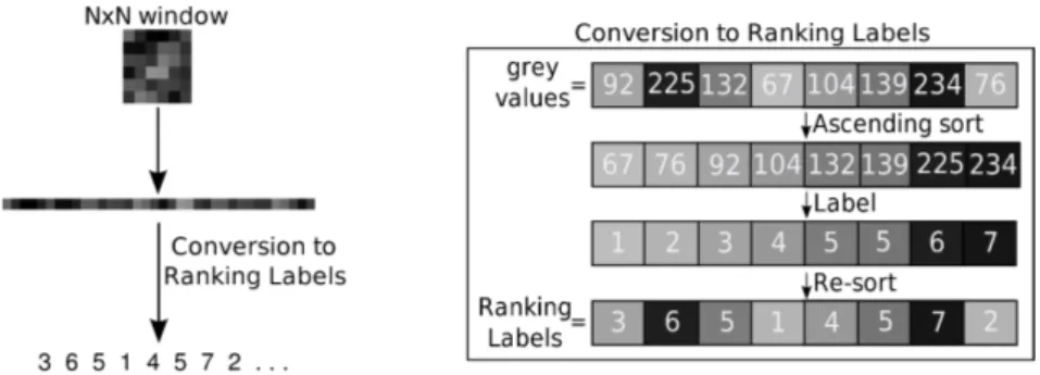
(3) Fig. 1. Example of the extraction process of Ranking Labels.. image, the rotation invariant uniform LBP (LBPri,u ) is supposed to provide a more accurate description of the face. As the quantity of LBPri,u is 9 in this case, a histogram of 10 bins describes each window. 2.2. Local Contrast Histograms. When computing the LBPs the information about the contrast in the window is lost. Therefore, local contrast histograms (LCH) can be used as an alternative feature set or combined together with LBPs in order to complement their characterization [7]. To compute the local contrast value of a pixel, a neighborhood is defined in a similar way as for LBP. Then the average of the grey level values of those neighbors that are brighter than the central pixel is subtracted from the average of the grey level values of the darker ones. Finally, all the local contrast values are accumulated in a histogram to obtain the LCHP,R . This notation means that the neighborhood used has P sample points on a circle of radius R. In order to have the same number of features as for the LBPs, when the neighborhood used has 8 samples points and its radius is 1 the LCH has 10 bins, whereas if the radius is 2 a 59-bin histogram is obtained. 2.3. Ranking Labels. In this description method a vector of ranking labels characterizes each window. For a N ×N window the values of the pixels within the window are substituted by their ranking positions. In other words, the grey level of each pixel is replaced by a numeric label that represents its position in the sorted list in ascending order of all grey levels within the window. This provides a more robust feature vector while keeping the positional information of each pixel inside the corresponding window. This characterization process is shown in Fig. 1 (see [8] for more detail).. 3. Experimental set-up. 3.1 General methodology The methodology designed uses the full-frontal face images from the FERET database [11], excluding those images where the person wears glasses. The images.

(4) used have been divided in two set: training and test with 60% and 40% of the images, respectively. It is worth noting that there are several images of the same person, but all of them are assigned to the same set of images. The methodology design is divided in the following steps: 1. The face is detected using the Viola and Jones algorithm [6] implemented in the OpenCV [12] library. This algorithm is completely automatic since only takes the image as input. The system does not correct the inclination that the face might have. 2. The top half of the resulting image from step 1 (the area of the image where the face was detected) is extracted and then equalized and resized to a preestablished smaller size. The interpolation process required for the resizing step uses a three-lobed Lanczos windowed sinc function [13] which keeps the original image aspect ratio. 3. A set of windows of N × N pixels are defined to obtain a collection of vectors that characterize the top half of the face. 4. Given a test image, the classification process consists of assigning to each vector the class label (female or male) of its nearest neighbor in the training set. The gender of a test face is obtained by one of these procedures: 1) by majority voting of all the labels of the face’s vectors or 2) by concatenating the vectors of all windows to build a longer vector to characterize the face, so the faces’s class label will be the same as its vector’s. The distance metrics used are the Euclidean metric and the Chi square metric and all the experiments have been done using both of them in order to compare which one performs better our task. 3.2. Description of the classification experiments. Four different experiments have been design to find out: 1) which is the face description that provides more information to discriminate between genders? and 2) which is the face description more suitable for situations where the face is not accurately detected? The details about the experiments are presented next: Experiment 1 In this case the top half face is split into a set of windows with no overlapping between them. This means that the pixels that belong to a window are never considered in another one. From each of the non-overlapping windows a feature vector is extracted. Then these vectors are concatenated to make a longer one. Hence, the vector of a certain window will be always compared with the vectors obtained from the windows that have the same position. Experiment 2 In order to extract more detailed features to describe the top half face, overlapping windows are used in this case. Therefore, one pixel will belong to several windows and its value will be used to obtain the descriptions of all of them. Although the size of the top half face images and the regions will be the same as in the previous experiment, the quantity of vectors will be higher because of.

(5) the overlapping. Finally, all the vectors are also concatenated to make only one longer vector and, therefore, the features of a certain window will be always compared with the features obtained from the windows that have the same position in the training images. Experiment 3 In this experiment the face is characterized by the same set of vectors obtained in experiment 2 but the classification process is different. Given a window of a test image, a set of neighboring windows will be considered in the training images. The size of that neighborhood depends on the error tolerance you may consider in the face detection process. The feature vector of the test window will be compared with the vectors obtained for all windows considered in the training images. The class label of the nearest neighbor is assigned to each window of the test face. Then, the test face obtains the class label resulting from the voting of all its windows. In our experiments the neighborhood considered is the whole face, so no precision is prefixed in the detection process. However, this approach leads to a high computational cost. Due to the fact that each vector is individually classified and its nearest neighbor is not restricted to those vectors obtained from the regions in the same position, faces will not need to be accurately detected as in the previous experiments. Experiment 4 This experiment presents a more realistic approach of the previous experiment. Now, the detection of the faces is artificially modified to simulate an inaccurate detection. The only difference with experiment 3 is that, after the automatic detection of the faces, a random displacement is applied to the area containing the face. The displacement could be at most 10% of the width for the horizontal movement and 10% of the height for the vertical one. This experiment allows us to test the face descriptions and the classification methods in a more unrestricted scenario. Consequently, it could provide more reliable results about whether our system would be suitable for situations where the face detection could not be accurate. 3.3. Development. A complete set of experiments (see Table 1) have been carried out to test the face descriptions described in Sect. 2 and several combinations of them. Specifically, the face descriptions implemented are the following: – Uniform LBP with neighborhoods of 8 sample points and radii 1 (LBPu8,1 ) and 2 (LBPu8,2 ). – The combination of the LBPu8,1 + LBPu8,2 which consists in concatenating the vectors obtained with both descriptions. – Local contrast histograms with neighborhoods of 8 sample points and radii 1 (LCH8,1 ) or 2 (LCH8,2 ). – The combination of LCH8,1 + LCH8,2 . – The combination of LBP and LCH with the same number of sample points and radius. The resulting face descriptions are: LBPu8,1 + LCH8,1 and LBPu8,2 + LCH8,2 ..

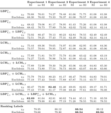
(6) Table 1. Recognition rates. Experiment 1 Experiment 2 Experiment 3 Experiment 4 RI no RI RI no RI RI no RI RI no RI LBPu 8,1. χ2 Euclidean. 70.88 68.30. 76.61 76.02. 74.27 73.33. 78.48 76.37. 61.66 61.08. 71.75 70.57. 61.08 61.08. 61.08 61.08. χ2 Euclidean. 68.42 68.42. 79.06 76.73. 81.17 77.89. 78.95 75.56. 61.43 62.02. 75.26 72.92. 61.08 62.14. 61.08 62.14. u LBPu 8,1 + LBP8,2 χ2 73.92 Euclidean 72.51. 80.47 78.25. 78.13 77.43. 80.23 77.31. 62.84 62.49. 78.55 76.32. 62.49 62.14. 62.49 62.14. LBPu 8,2. LCH8,1 χ2 Euclidean. 75.44 73.57. 69.36 70.64. 79.65 78.95. 74.97 72.87. 61.08 61.08. 62.95 64.36. 61.08 61.08. 64.36 65.06. χ2 Euclidean. 77.89 74.27. 71.81 72.05. 79.77 76.96. 75.79 74.50. 61.08 61.08. 63.42 63.42. 61.08 61.08. 63.19 64.13. LCH8,1 + LCH8,2 χ2 77.89 Euclidean 75.44. 72.98 73.80. 79.30 77.54. 76.26 76.73. 65.06 66.00. 64.48 63.07. 64.83 64.48. 65.30 63.66. LBPu 8,1 + LCH8,1 χ2 75.79 Euclidean 77.19. 79.53 77.43. 80.23 79.65. 81.17 77.89. 66.47 67.87. 79.95 75.15. 64.83 65.77. 79.01 73.51. LBPu 8,2 + LCH8,2 χ2 80.47 Euclidean 77.43. 79.88 77.66. 82.46 81.17. 81.40 77.08. 69.05 69.40. 82.65 77.61. 69.17 69.64. 81.71 76.08. 80.82 77.19. 74.44 71.28. 85.11 78.55. 71.16 70.81. 83.59 78.55. LCH8,2. u LBPu 8,1 + LCH8,1 + LBP8,2 + LCH8,2. χ2 Euclidean Ranking Labels χ2 Euclidean. 82.69 80.70. 81.64 79.88. 82.81 81.40. 78.95 78.60. 80.12 79.30. 88.54 88.54. 89.12 89.94. – The combination of the two previous which results in LBPu8,1 + LCH8,1 + LBPu8,2 + LCH8,2 . – Ranking labels description. All the face descriptions based on LBPs, produced two experiments: one with the sensitive to rotation version and the other one with the rotationally invariant version. In case of sensitive to rotation descriptions the vectors produced are composed of 10 features, while on the other case the vectors have 59 elements. Ranking labels description produces 49 features vectors. In all the experiments, the amount of images used was 2147. The top half face images were reduced to a 45 × 18 pixels image. The size of the window that scans the images is 7 × 7 in all cases.. 4. Results and Discussion. The correct classification rates obtained for each experiment carried out are shown in Table 1..

(7) With regard to the distance metrics used, the Chi square succeeded in recognizing the genders with better rates than the Euclidean metric in 73% of the cases. Concerning the radius of the neighborhood used for the histogram based features, radius 2 performs the recognition task better than radius 1 in 81% of the cases. Nevertheless, the combination of the same face description using both radii achieves higher rates, but using twice as many features. As can be easily seen, the sensitive to rotation descriptions achieved better results than the rotationally invariant ones when only the LBPs are used. However, the use of 59-bin histograms to describe the LCH provided worse results in experiments 1 and 2. This could be explained by the higher dispersion of the data which leads to a poorer characterization which also causes lower recognition rates in most of the cases that combined LBP and LCH. The results of experiments 1 and 2 show that the LCH is really useful to discriminate between genders since recognition rates reached by the LCH are very similar to those achieve using the LBP. LCH performs better when using rotationally invariant descriptions, whereas the rates obtained using LBP are slightly higher when the rotation dependent features were considered. As expected, when the LBP and the LCH with the radii 1 and 2 are used together to describe the faces, the recognition rate goes up until 82.69% (experiment 1) and 82.81% (experiment 2) which are the best rates of these experiment. However, the ranking label description achieved the best results when individual features were considered (not combinations of several features). To summarize, experiments 1 and 2 have proved that all the face descriptions are quite good to discriminate between genders. Not very important differences were obtained in the classification rates. In general, the more number of features used to describe the faces, the best classification rates obtained. For experiments 3 and 4, the ranking labels description was the most suitable since it reached the best recognition rates which were close to 90%. That is, the correct classification rates were even better than for experiments 1 and 2. In our opinion, this is due to the fact that experiments 1 and 2 considered that the faces have always been perfectly located in the images. The error tolerance introduced in the classification experiments 3 and 4 helped to improve the rates obtained as they avoided the influence of the localization errors. However, this significant improvement only happens for the ranking labels features. Features based on individual histograms performed in these cases worse than for experiments 1 and 2. This is probably because the ranking label features keep the positional information of each pixel inside the corresponding window. Therefore, they keep their discriminative power even when the features of a certain window are compared against the features of another window which is located at a different spatial position. However, histogram based features required this correspondence between windows in the test and training images in order to keep their performance. Combining all histogram-based features, the classification rates also improved slightly, but using a very high number of features per window..

(8) 5. Conclusions. This paper has addressed the automatic gender classification problem in situations where the face was partially occluded and inaccurately detected. The experiments have shown that LBPs and LCHs performed correctly when the positional information is kept by the classification method. However, these face descriptions are less reliable in situations with non-accurate face detections, since there is an important spatial information loss. The best characterization method in an inaccurate environment was the ranking labels description which reached to almost a 90% of recognition rate due to the fact that these features were designed to keep the information about the position of the pixels in the different windows considered over the image. Summing up, ranking labels are the most reliable characterization method as it performs in a similar way in all experiments carried out. Although, LBPs and LCHs performed correctly the gender recognition task, they were more dependent on the accuracy of the face localization process.. References 1. Rajagopalan, A.N., Rao, K.S., Kumar, Y.A.: Face recognition using multiple facial features. Pattern Recogn. Lett. 28(3) (2007) 335–341 2. Ahonen, T., Hadid, A., Pietikainen, M.: Face description with local binary patterns: Application to face recognition. Pattern Analysis and Machine Intelligence, IEEE Transactions on 28(12) (2006) 2037–2041 3. Brubaker, S.C., Wu, J., Sun, J., Mullin, M.D., Rehg, J.M.: On the design of cascades of boosted ensembles for face detection. Int. J. Comput. Vision 77(1-3) (2008) 65–86 4. Chang Huang, Haizhou Ai, Y.L., Lao, S.: High-performance rotation invariant multiview face detection. Pattern Analysis and Machine Intelligence, IEEE Transactions on 29(4) (2007) 671–686 5. Garcia, C., Delakis, M.: Convolutional face finder: a neural architecture for fast and robust face detection. Pattern Analysis and Machine Intelligence, IEEE Transactions on 26(11) (2004) 1408–1423 6. Viola, P., Jones, M.: Robust real-time face detection. International Journal of Computer Vision 57 (2004) 137–154 7. Ahonen, T., Pietikainen, M., Harwood, D.: A comparative study of texture measures with classification based on featured distributions. Pattern Recognition 29(1) (1996) 51–59 8. Andreu Y., Mollineda, R., P., G.S.: Gender recognition from a partial view of the face using local feature vectors. In: Proc. of The Iberian Conf. on Pattern Recognition and Image Analysis (IbPRIA’09). LNCS (2009) 481–488 9. Topi, M., Timo, O., Matti, P., Maricor, S.: Robust texture classification by subsets of local binary patterns. Volume 3. (2000) 935–938 vol.3 10. Ojala, T., Pietikäinen, M., Mäenpää, T.: Multiresolution gray-scale and rotation invariant texture classification with local binary patterns. IEEE Trans. Pattern Anal. Mach. Intell. 24(7) (2002) 971–987 11. Phillips, H., Moon, P., Rizvi, S.: The FERET evaluation methodology for face recognition algorithms. IEEE Trans. on PAMI 22(10) (2000) 12. Bradski, G.R., Kaehler, A.: Learning OpenCV. O’Reilly (2008) 13. Turkowski, K.: Filters for common resampling tasks. (1990) 147–165.

(9)